ADMM-Based Discriminative Shape Segmentation with Loopy Part ...

Fast and Exact: ADMM-Based Discriminative Shape Segmentation with Loopy Part Models Haithem Boussaid ∗, Iasonas Kokkinos Center for Visual Computing, Ecole Centrale de Paris, France INRIA - Galen Team, Saclay, Ile-de-France Unit {haithem.boussaid, iasonas.kokkinos}@ecp.fr

Ini.al  solu.on  (t=1)   Master  

Abstract In this work we use loopy part models to segment ensembles of organs in medical images. Each organ’s shape is represented as a cyclic graph, while shape consistency is enforced through inter-shape connections. Our contributions are two-fold: firstly, we use an efficient decomposition-coordination algorithm to solve the resulting optimization problems: we decompose the model’s graph into a set of open, chain-structured, graphs each of which is efficiently optimized using Dynamic Programming with Generalized Distance Transforms. We use the Alternating Direction Method of Multipliers (ADMM) to fix the potential inconsistencies of the individual solutions and show that ADMM yields substantially faster convergence than plain Dual Decomposition-based methods. Secondly, we employ structured prediction to encompass loss functions that better reflect the performance criteria used in medical image segmentation. By using the mean contour distance (MCD) as a structured loss during training, we obtain clear test-time performance gains. We demonstrate the merits of exact and efficient inference with rich, structured models in a large X-Ray image segmentation benchmark, where we obtain systematic improvements over the current state-of-the-art.

ADMM  

Slave  1  

Slaves  

Final  solu.on  (t=8)  

Slave  N  

…  

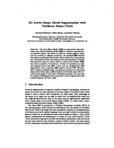
Figure 1. ADMM optimization for shape segmentation with loopy part models: loopy graphs can encode shape constraints (closure, inter-organ dependecies), but yield hard optimization problems. We decompose the original, loopy optimization problem into a subset of easier, loop-free problems (slaves), and use a ‘master’ procedure to ensure consistency. At each iteration, every slave i communicates its solution Xi to the master; the master then detects inconsistencies in the individual slave solutions (indicated by red arrows) and drives the slaves towards a consistent solution in the next iteration, py passing parameters u(r), λi (r) that affect the slave problems around the common nodes, r. ADMM quickly leads to consensus among the different slaves, as shown on the right: the dual and the primal problems reach a zero duality gap in a small number of iterations. The estimated organ boundaries closely match the color-coded ground truth organ segmentation.

1. Introduction

ignored in performance evaluation. Here instead we use deformable models in a setting similar to human pose estimation [1, 33, 34] where accurate body part estimation is the main goal. Our goal is to segment ensembles of shapes in medical images: this involves outlining the boundaries of medical organs, while potentially exploiting inter-organ dependencies to transfer information from clearly visible parts to harder areas. Apart from the obvious societal impact of medical imaging, what we find most interesting in this problem is the complexity, and accuracy of the annotation being employed

Deformable part models (DPMs) are ubiquitous in computer vision, and are currently being used in a broad range of high-level tasks, including object detection [14, 16], pose estimation [1, 33, 34] and facial landmark localization [47]. When deformable models are used to detect objects, deformations are treated as a hurdle, that must be done away with, in order to achieve robust detection: during training, deformations are commonly treated as latent variables, and ∗ This work was supported by grant ANR-10-JCJC-0205 (HiCoRe) and the EU-FP7 project RECONFIG.

1

-we have 196 landmarks, localized by expert physicians. Such datasets provide a challenging testbed for algorithm assessment, while with the advent of strongly supervised object annotations [2, 5, 41] we anticipate that our advances will become increasingly relevant to recognition. In this work we cast multi-organ shape segmentation and landmark localization in a graphical model framework, and present advances on both the optimization and learning side. In particular, we represent every organ as a cyclic graph, whose nodes indicate landmarks positions. Importantly, we use loopy graphs to incorporate problem constraints (e.g. contour closedness and relative shape positions) that cannot be encoded through chain- or tree- structured graphs. This directly raises the computational efficiency issue addressing which is a main contribution of this work. In our case we have many (196) nodes and a label space in the order of tens, or hundreds of thousands of values, corresponding to discretized 2D positions. To deal with the complexity of optimization we first constrain our models to use separable quadratic pairwise terms; as such, we can use Generalized Distance Transforms (GDTs) [17, 14] to perform Dynamic Programming (DP) with complexity that is linear rather than quadratic in the number of pixels. We couple GDT-based DP with a coordinationdecomposition scheme akin to Dual Decomposition (DD) [25, 3, 37]: we rewrite the score of our graphical model as a sum of score functions defined on overlapping chain graphs (slaves), perform inference efficiently for every chain, and use an iterative master-slave scheme to enforce that the computed solutions are consistent. Earlier works [34] have reported that when implemented for spatial variables Dual Decomposition is slow, or does not converge (500 iterations were used in [34]). We have observed this is true if we use a simple subgradient-based implementation; however by using the Alternation Direction Method of Multipliers (ADMM) [8, 27] we achieve convergence in a few (typically less than 10) iterations, even when sharing multiple (30) nodes among the slaves. Our second contribution lies in introducing a structured prediction framework suited to the task at hand. In particular, we use structural SVMs to optimize a loss function specific to contours, considering the minimization of the mean contour distance performance measure (MCD). The resulting learned score function allows us to rank each candidate contour according to its MCD to the ground truth configuration, and lends itself to straightforward inclusion into structured prediction learning by virtue of being decomposable into a sum over landmark nodes. In Sec. 6 we demonstrate the merit of our contributions using the Segmentation in Chest Radiographs (SCR) benchmark [36, 40]. As baseline we use a recent model of ours [7], that employs chain-structured graphs, and is trained with the standard zero-one loss; this already out-

performed the current state-of-the-art in medical image segmentation, by virtue of its end-to-end discriminative training. As demonstrated by a host of evaluation measures, including the Mean Contour Distance, the Dice and the Jaccard coefficient, each of the above steps adds to our model’s performance. Our implementation will be made available from cvn. ecp.fr/personnel/haithem/.

2. Prior work Deformable contour models (DCMs) have been used to localize boundaries in medical images starting from the seminal works of Snakes [22], Deformable Templates [46] and Active Shape/Appearance Models [11, 12], also known as point distribution models; a rich set of works revolved around the reformulation of DCMs in intrinsic geometric terms [9] and the introduction of statistical shape priors [26, 31, 10, 13] in curve evolution. Complementary to this has been the incorporation of richer, landmark-specific local terms [35, 29, 30, 4] instead of the simpler gradientbased terms used in earlier works such as [9, 31]. Finally, star-shaped graphical models [14, 15] have been adopted to organ detection in [29, 30, 4], while recently SIFT-like features have been used for shape matching in both the sparse [38, 4], and dense settings [29, 30]. Even though these works revolve around the theme of learning for shape matching in medical imaging, to the best of our understanding, none is trained in a integrated, endto-end manner. Having started with this task in the simplest setting in [7], in this work we move on towards more challenging and interesting inference and learning problems.

2.1. Dual Decomposition and ADMM in vision As will be detailed in Section 4, one of our main technical contributions consists in introducing ADMM to inference in loopy graphs with large label spaces, corresponding to discretized spatial variables. ADMM can be understood as a generalization of Dual Decomposition (DD) [25, 3, 37] which in turn is already extensively used in vision and medical image segmentation [43, 42, 44]. ADMM has found tremendous success in image processing/compressed sensing, commonly under the name of ‘Bregman iteration’ methods [19, 45]. In connection with optimization problems revolving around MRFs, ADMM has recently been used in conjunction with discrete MRFs [27], but little work has been done for MRFs with large/continuous label spaces. Recently [32] used ADMM to perform inference with polynomial energies in continuous graphical models, by iteratively linearizing a cost function used for registration; this was done to constrain the energy function to be polynomial in the unary terms. This is however not an option for our case, where we want to match deformable shapes to

1

5

1

1

5

5

xj = (hj , vj ) with a quadratic expression of the form: T

2

6

2

2

6

6

3

7

3

3

7

7

Vi,j (xi , xj )=− (xj −xi −µi,j ) Ci,j (xj − xi − µi,j ) , (3) where Ci,j = diag(νi , ηi ) is a diagonal matrix and µi,j = ¯ v¯)T is the nominal displacement between xi and xj . (h, The form of Ci,j allows us to write the pairwise term as a function separable in h and v: Vi,j (xi , xj )

4

8

4

4

8

8

Figure 2. We decompose energy functions on loopy graphs into functions on chain-structured subgraphs, and use the latter as slaves in a decomposition-coordination optimization algorithm. Shown in (a) is an example of a complex graph involving a ‘zipper’ chain between shapes (e.g. nodes 1-4 can belong to the lung, and nodes 5-8 to the heart) and in (b) the decomposition of the complex graph into chain structured subproblems.

unconstrained images - where the unary terms are far from linear, or convex. Earlier works on applying DD in a setting similar to ours [34] had concluded that DD converges very slowly, which we also observed empirically; by contrast we show that ADMM typically converges in less than 10 iteations, commonly attaining a duality gap equal to zero.

3. Merit Function Formulation Our shape representation involves a set of K anatomical landmarks: X = {x1 , . . . , xK }, where every landmark’s position is described by a 2D position vector xi = (hi , vi ); we denote vectors with boldface letters and will alternate between the vector notation x and the horizontal/vertical notation (h, v) based on convenience. Given an image I we score a landmark configuration X with a merit function S formed as the sum of unary and pairwise terms: SI (X) =

K X i=1

UI,i (xi ) +

X

Vi,j (xi , xj ),

(1)

i,j∈E

where E is the set of edges on the graph. The unary terms capture the local fidelity of the image observations at xi to a landmark-specific appearance model Ui , in terms of an inner product between a weight vector ui and dense image features extracted around every point xi : UI,i (xi ) = hui , fI (xi )i.

(2)

We denote by fI (xi ) : R2 → RD a ’dense’ mapping from image coordinates to D-dimensional features; as detailed in Sec. 6, we experiment with Daisy [39] and dense SIFT [18]. The pairwise term Vi,j (xi , xj ) constrains the location xi = (hi , vi ) of landmark i with respect to its neighbor

= hvi,j , p(xi , xj )i,

vi,j =

(4)

(νi , ηj ),

(5) 2 2 ¯ p(xi , xj ) = (−(hj − hi − h) ,−(vj −vi − v¯) ).(6) Having written the pairwise terms as the inner product between a weight and a feature vector, and given that the unary terms are also inner products between weights and features, it follows that Eq. 1 can be written as: SI (X, w) = hw, hI (X)i,

where

(7)

w = (ui , vi,j ) hI (X) = (fI (xi ), p(xi , xj ), i, j ∈ E (8) We will write SI (X, w) to stress that SI (X) depends on w.

4. ADMM for Inference in Loopy Graphs The model outlined above makes no assumption about the model structure, and as such can contain loops; this may directly reflect the problem structure (e.g. the closedness constraint of a region’s boundary), but when working with spatial variables in a large label space it is practically prohibitive to work even with the easiest loopy graphs; even if the graph’s treewidth is two, the complexity of MAP inference grows by O(N 3 ) where N is the number of pixels. We address this problem by building on the Dual Decomposition (DD) technique [3, 25], and in particular its acceleration attained with the Alternating Direction Method of Multipliers [8, 28]. This combines the benefits of DD [3] (fast optimization of the slave problems) and ADMM (rapid convergence) in a seamless manner, without practically altering the optimization procedure for the slaves. We now describe how we use ADMM for our problem. Our goal is, given an image I to solve: X∗I = argmax SI (X, w).

(9)

X

Dual Decomposition proceeds by rewriting the score SI of our graphical model as a sum of score functions Si defined on overlapping subgraphs (slaves), S(X) = PN i=1 Si (X), allowing (temporarily) each slave to have its own solution, Xi , but adding the constraint that, on common nodes, different slaves must have identical solutions. As illustrated in Fig. 2, in our problem we break every closed contour into two open chains that overlap at their end and start nodes, and introduce ‘zipper’ chains among

organs that share edges, where the ‘zipper’ passes through the intra-organ edges. These are the slave problems Si of our problem. Denoting by R ⊂ 1..K the subset of point indices belonging to more than one chain model, our inference problem becomes: maxS(X) =

N X

Si (Xi ) s.t.Xi (r) = u(r) ∀r ∈ R (10)

i=1

where X = {Xi }, i = 1 . . . N is the ensemble of slave solutions and u(r) ensures consistency at overlapping points. Dual Decomposition relaxes the constraints in Eq. 10 by introducing a Lagrange multiplier λi (r) for each agreement constraint. ADMM adds a quadratic penalty for constraint violation, yielding the augmented Lagrangian: A(X, u, λ) = −

N X

X

i=1

r∈R

(Si (Xi ) +

λi (r)Xi (r)) (11)

X X XX ( λi (r))u(r) − ρ (Xi (r) − u(r))2 r∈R

i

i

r

where ρ is a positive parameter that controls the intensity of the augmenting penalty (we note that we deviate a bit from the common presentaton of the method, e.g. [8], as we phrase our original problem as one of maximization rather than minimization). To find an extremum of the augmented Lagrangian, ADMM iterates the following steps: Xt+1 i

=

ut+1

=

argmax A(Xi , ut , λt )

(12)

Xi

argmax A({Xt+1 }, u, λt ) i

(13)

u

λt+1 (r) i

=

Figure 3. Evolution of the dual objective and the primal one as a function of DD/ADMM iterations. ADMM-based optimization rapidly converges, achieving a duality gap of zero typically in less than 20 iterations. Subgradient based method does not converge even after 100 iterations. These results are obtained by averaging over hundred different example images.

λti (r) − αt (Xt+1 (r) − ut+1 (r)) (14) i

In words, the slaves efficiently solve their sub-problems (Eq. 12), and deliver Xi to the master. The master then coordinates the individual solutions, by updating the current multipliers λt+1 (r) (Eq. 14) and ut+1 (r) (Eq. 13), and i communicating them to the slaves for the next iteration. We observe that solving Eq. 12 for a given i amounts to solving independently for a chain structured model. We can verify that the effect of the (augmented) Lagrangian function on the individual subproblems is absorbed by updating the unary terms of the slaves with a parametric, quadratic function of position; since the slaves are chain-structured, means we can still efficiently optimize them with GDTs. As shown in Fig. 3, ADMM is dramatically faster than Dual Decomposition for our problem. For our full-blown model, involving |R| = 30 shared nodes in Eq. 10, Dual Decomposition would often not converge even after 100 iterations, while we obtained convergence of ADMM in typically no more than 20 iterations. This means that the effective complexity of our joint inference algorithm in loopy

graphs is linear in the number of pixels, since every slave can be optimized in linear time with GDTs. We note that ADMM is guaranteed to converge to the global optimum only if the score function being maximized is concave. In our case, this is not guaranteed (the unary terms are arbitrary), so we can understand ADMM only as an approximate optimization algorithm. The fact that we have a zero duality gap at convergence indicates that for the examples considered in our experiments approximate inference delivers the exact solution. Finally, before moving on to learning, we note that we accommodate global scale changes through multiresolution optimization; from our original image I we construct an image pyramid by resampling at a set of scales S = (1, r, r2 , . . . , rS ) and compute: X∗I,S = argmax sI(ri ) (X, w),

(15)

X,i

where I(ri ) denotes the image resampled with a ratio ri . For notational convenience we will drop the S subscript from now on and it will be implied that the result is obtained through a multi-scale optimization.

5. Structured Prediction for Segmentation We assume that we have been provided with a training set of images and associated ground-truth contour locations, ˆ i )}, i = 1 . . . N . We which we will denote as X = {(Ii , X recall that our merit function SIi (X, w) is an inner product between a weight vector w and a feature vector hIi (X). As is common in structured prediction, [21], we measure the

performance of a particular weight vector in terms of a loss ˆi ) which represents the cost incurred by function ∆(X∗Ii , X ˆi . labelling image i as X∗Ii when the ground truth is X The simplest option we consider is the general 0-1 loss:  ˆ 0, X = X ˆ = ∆0−1 (X, X) (16) 1, otherwise. which penalizes any discrepancy between the ground truth and the recovered solution. Different loss functions can be used however to better reflect the nature of our problem. In particular we use the Mean Contour Distance (MCD) which measures the average distance of the landmarks of two contours. In our case, the contours are discretized to a set of landmark positions, connected through straight lines. ˆ is defined as: The MCD between two contours X and X K X ˆ = 1 ˆ i ||2 . ||xi − x ∆mcd (X, X) K i=1

(17)

For cutting plane training of structural SVMs [21] we need, given the current value of w, to find a Xicp that has good score according to the model, and a high loss according to the ground-truth; for our case, this results in the problem: Xicp

=

ˆ i ). argmax sIi (X, w) + ∆(X, X

(18)

X

For the loss in Eq. 17, finding the most violated constraint is equivalent to the following modified inference problem: Xicp=argmax X

K X k=1

ˆ k ))+ (UIi ,k (xk )+δ(xk , x

X

Vk (xk , xj ),

(k,j)∈E

1 ˆi) = K ˆ i ||2 is the per-landmark dewhere δ(xi , x ||xi − x composition of the loss; since this term is absorbed in the unary term, it follows that optimizing this last expression can be done as efficiently as solving the original optimization problem.

6. Experimental Settings and Results In all of our experiments we use the publicly available dataset and evaluation setup described in [36, 40]; this dataset contains 247 standard posterior anterior chest radiographs of healthy and non-healthy subjects presenting nodules. The database contains gold standard segmentations from radiologists that provided a delineation of the lung fields, the heart and the clavicles. Gold standard segmentation masks are hence available as well as corresponding landmark positions lying on the contour. Following the evaluation setup described in [36], we use 123 images for training and a separate set of 124 images for testing, using the provided training/testing split; all of the

Figure 4. Our graphical model’s topology reflects the placement of multiple organs corresponding to a patient’s heart, lungs, and clavicles. In the detail (right) we are showing in black the edges used to connect the left clavicle and the left lung, as well as the edge that makes the lung contour closed.

reported results are on the whole test set, using images of size 256 by 256. Our model contains 196 nodes including 30 shared nodes. We have 16 slave problems, 2 per organ plus 26 for the links (’zipper’ contours). For ADMM we found that we achieve fastest convergence when setting ρ = 1 in 12 and setting the step size αt to follow a non-summable diminishing step length rule, as detailed in [3]. Since our code will be publicly available, we refrain from thoroughly presenting implementation details. Starting with computational efficiency, for our problem the computation of unary terms requires 0.4 seconds on a standard PC; each slave problem takes 0.06 seconds per contour and scale, for a contour with 20 nodes; for 8 contours and 7 scales, this means 3.4 seconds per iteration of ADMM/Dual Decomposition. ADMM/DD take practically the same time per iteration, but ADMM converges in less than 20 iterations (typically 10) while DD did not converge even after 100 iterations. Turning to accuracy, we first note that both optimization and learning do not suffer from local minima issues, while the complexity penalty coefficient of structured SVM is determined with 10-fold cross validation; we can thus attribute any difference in the final results exclusively to the lowlevel feature, model structure, and loss function choices. In particular in Table 1 we compare the segmentations delivered by different design choices to the ground truth using the Dice and Jaccard area overlap coefficients and the Mean Contour Distance, as defined in [40]. Our design choices include (a) the use of different low-level features, comparing Daisy features [39] and Dense SIFT [18] computed at different scales (b) graph topology, comparing our earlier chain-graph baseline (CG) [7], to the use of a loopy graph (LG) and (c) the use of the 0-1 loss versus the use of the MCD loss during training. Our very first observation is that our baseline outperforms the previous state-of-the-art in medical imaging, and with a large margin. We further verify (i) that the use of

a

b c (a,b): chain graph (baseline). (c,d): loopy-graph results (ADMM results).

d

Figure 5. Segmentation results on lungs, heart and clavicles. Ground truth contours are shown in green, our results are shown in other colors. We observe that the loopy-graph model delivers more accurate results that stick more closely to the ground truth annotations. We attribute this to the ability of our loopy-graph model to account for closedness constraints, and also to model interactions among multiple parts - for instance that the clavicle boundaries need to be at a prescribed distance from the lung boundaries.

Figure 6. Dice coefficients (left) and Mean Contour Distance statistics (right) on different chest organs (the overall decrease in the DICE coefficients for the clavicles is anticipated due to their smaller scale).

Table 1. Performance measures for the previous state-of-the-art of [35], and different choices for our method, involving Daisy features, dense SIFT at a resolution of 4, and 8 pixels per bin, the use of chain graphs (CG suffix) vs. loopy graphs (LG suffix), and the use of the MCD loss for training (MCD suffix). method [35, 40] Daisy+CG Daisy+LG Daisy+LG+MCD Sift-4+CG Sift-4+LG Sift-4+LG+MCD Sift-8+CG Sift-8+LG Sift-8+LG+MCD

Right Lung (44 points) Dice Jacc. mcd N/A 94.0 1.5 97.97 96.0 1.2 98.1 96.27 1.3 98.24 96.54 1.0 97.54 95.2 1.5 97.35 94.84 1.7 97.88 95.85 0.9 97.71 95.52 1.5 97.68 95.47 1.3 98.00 96.1 0.9

Left Lung (50 points) Dice Jacc. mcd N/A 92.0 1.7 97.52 95.2 1.4 97.66 95 1.2 97.89 95.9 1.7 96.8 93.6 1.8 97.52 95.2 1.4 97.8 95.7 1.9 97.00 94.1 2.0 97.28 94.6 1.5 97.9 95.9 1.4

Heart (26 points) Dice Jacc. mcd N/A 88.0 3.5 95 91.3 2.3 96.5 93.2 1.3 96.84 93.9 1.7 94.3 91.3 2.3 96.17 92.6 2.7 96.95 94.5 1.8 95 90.7 2.3 95.81 91.1 2.8 96.20 92.7 1.7

Table 2. Pixel error results on the SCR database [36, 40]. The proposed method scores better than the state-of-the art approaches.

method Our [7] MISCP [35] ASM tuned [40]

pixel error 0.017±0.008 0.022±0.006 0.033±0.017 0.044±0.014

loopy models improves performance and (ii) that the use of the MCD loss improves performance as well. These results are consistently supported practically by all organs, evaluation measures, and front-end feature choices. Optimizing the MCD loss during training further improves the performance of our system. This is reflected by the clear boost in performance versus the 0-1 loss training, as assessed by the MCD validation measure on the test set. The results in Table 1 are complemented by the results in Fig. 6 where we provide box plots of different validation measures for the different organs that we work with. Moreover, we compare in Table 2 our pixel error results with the current state-of-the-art results on the same dataset [40, 35]. We further verify through a paired T test [20] that the pixel error improvement is statically significant (p=0.04). We validate hence again that structured prediction with the MCD loss coupled with a loopy model results in clear, systematic improvements over the state-of-the-art for all of the organs that we consider in our evaluation. Finally, a side-by-side comparison of our baseline model and the full-blown, loopy-graph model developed in this paper is provided in Fig. 5, which qualitatively demonstrates the higher accuracy attained by our model on challenging areas with poor low-level information. Some notable cases include the case of the heart, where the added geometric constraint allows us to recover from unary detector failure in the blank area.

7. Discussion In this work, we developed an efficient technique to performing inference on loopy graphs with spatial variables,

Right Clavicle (23 points) Dice Jacc. mcd N/A 78.7 2 90.4 82.48 1.8 91.8 84.84 1.7 93.04 86.99 1.5 89.9 81.65 1.9 92.04 85.25 2 92.89 86.72 1.6 90.00 81.82 1.9 91.75 84.76 1.9 92.8 86.57 1.7

left Clavicle (23 points) Dice Jacc. mcd N/A 75.8 2 88.11 78.75 2.3 89.19 80.5 2 89.95 81.9 1.8 88.1 78.73 1.8 88.85 79.9 1.8 89.6 81.2 1.5 87.4 77.6 2.8 89.22 80.6 1.9 89.8 81.5 1.4

by employing the Alternating Directions Method of Multipliers (ADMM) in conjunction with Generalized Distance Transforms (GDTs) and introduced a structured prediction approach to the task of learning to segment multiple organs from medical images. We demonstrated systematic improvements over the current state-of-the-art in medical image segmentation, both due to the use of richer models, and better adapted score functions, trained with structured prediction. On the efficient optimization side we intend to pursue further acceleration by exploiting recent advances on fast DPM detection using Branch-and-Bound [23, 24] in conjunction with 3D optimization problems [6]. On the learning side we intend to further pursue the learning of loopy graph models for other shape matching tasks, such as face recognition and body pose estimation, where matching accuracy is of importance [1, 33, 34, 5]; with the advent of strongly-supervised datasets [2, 41] we anticipate that this will become increasingly central to high-level vision tasks, such as object detection.

References [1] M. Andriluka, S. Roth, and B. Schiele. Discriminative appearance models for pictorial structures. IJCV, 99(3):259– 280, 2012. 1, 7 [2] H. Azizpour and I. Laptev. Object detection using stronglysupervised deformable part models. In ECCV, 2012. 2, 7 [3] D. P. Bertsekas. Nonlinear Programming. Athena Scientific, 1999. 2, 3, 5 [4] A. Besbes and N. Paragios. Landmark-based segmentation of lungs while handling partial correspondences using sparse graph-based priors. In ISBI, 2011. 2 [5] L. Bourdev and J. Malik. Poselets: Body part detectors trained using 3d human pose annotations. In ICCV, 2009. 2, 7 [6] H. Boussaid, I. Kokkinos, and N. Paragios. Rapid mode estimation for 3d brain mri tumor segmentation. In EMMCVPR, 2013. 7

[7] H. Boussaid, I. Kokkinos, and N. Paragios. Discriminative learning of deformable contour models. In ISBI, 2014. 2, 5, 7 [8] S. P. Boyd, N. Parikh, E. Chu, B. Peleato, and J. Eckstein. Distributed optimization and statistical learning via the alternating direction method of multipliers. Foundations and Trends in Machine Learning, 3(1):1–122, 2011. 2, 3, 4 [9] V. Caselles, R. Kimmel, and G. Sapiro. Geodesic Active Contours. IJCV, 22(1):61–79, 1997. 2 [10] Y. Chen, S. Thriuvenkadam, H. Tagare, F. Huang, D. Wilson, and E. Geiser. On the Incorporation of Shape Priors into Geometric Active Contours. In VLSM Workshop, 2001. 2 [11] T. Cootes, G. J. Edwards, and C. Taylor. Active Appearance Models. In ECCV, 1998. 2 [12] T. F. Cootes, C. J. Taylor, D. H. Cooper, and J. Graham. Active shape models-their training and application. CVIU, 61:38–59, 1995. 2 [13] D. Cremers. Dynamical statistical shape priors for level set based tracking. Trans. PAMI, 2006. 2 [14] P. Felzenszwalb and D. Huttenlocher. Pictorial Structures for Object Recognition. IJCV, 61(1):55–79, 2005. 1, 2 [15] P. Felzenszwalb, D. McAllester, and D. Ramanan. A discriminatively trained, multiscale, deformable part model. In CVPR, 2008. 2 [16] P. F. Felzenszwalb, R. B. Girshick, and D. A. McAllester. Cascade object detection with deformable part models. In CVPR, 2010. 1 [17] P. F. Felzenszwalb and D. P. Huttenlocher. Distance transforms of sampled functions. Technical report, 2004. 2 [18] B. Fulkerson, A. Vedaldi, and S. Soatto. Localizing objects with smart dictionaries. In ECCV, 2008. 3, 5 [19] T. Goldstein and S. Osher. The split bregman method for l1-regularized problems. SIAM J. Imaging Sciences, 2009. 2 [20] C. H. Goulden. Methods of Statistical Analysis. 2008. 7 [21] T. Joachims, T. Finley, and C.-N. J. Yu. Cutting-plane training of structural svms. Machine Learning. 4, 5 [22] M. Kass, A. Witkin, and D. Terzopoulos. Snakes: Active Contour Models. In ICCV, 1987. 2 [23] I. Kokkinos. Rapid deformable object detection using dualtree branch-and-bound. In NIPS, 2011. 7 [24] I. Kokkinos. Shufflets: Shared mid-level parts for fast object detection. In ICCV, 2013. 7 [25] N. Komodakis, N. Paragios, and G. Tziritas. Mrf optimization via dual decomposition: Message-passing revisited. In ICCV, 2007. 2, 3 [26] M. Leventon, O. Faugeras, and E. Grimson. Statistical Shape Influence in Geodesic Active Contours. In CVPR, 2000. 2 [27] A. Martins, M. Figueiredo, P. Aguiar, N. Smith, and E. Xing. An augmented lagrangian approach to constrained map inference. In ICML, 2011. 2 [28] A. F. T. Martins, N. A. Smith, P. M. Q. Aguiar, and M. A. T. Figueiredo. Dual decomposition with many overlapping components. In EMNLP, 2011. 3 [29] V. Potesil, T. Kadir, G. Platsch, and M. Brady. Improved anatomical landmark localization in medical images using dense matching of graphical models. In BMVC, 2010. 2

[30] V. Potesil, T. Kadir, G. Platsch, and M. Brady. Personalization of pictorial structures for anatomical landmark localization. In IPMI, 2011. 2 [31] M. Rousson and N. Paragios. Shape Priors for Level Set Representations. In ECCV, 2002. 2 [32] M. Salzmann. Continuous inference in graphical models with polynomial energies. In CVPR, 2013. 2 [33] B. Sapp, A. Toshev, and B. Taskar. Cascaded models for articulated pose estimation. In ECCV, 2010. 1, 7 [34] B. Sapp, D. Weiss, and B. Taskar. Parsing human motion with stretchable models. In CVPR, 2011. 1, 2, 3, 7 [35] D. Seghers, D. Loeckx, F. Maes, D. Vandermeulen, and P. Suetens. Minimal shape and intensity cost path segmentation. IEEE Trans. Med. Imaging, 2007. 2, 7 [36] J. Shiraishi, S. Katsuragawa, T. M. J. Ikezoe, T. Kobayashi, K. Komatsu, M. Matsui, H. Fujita, Y. Kodera, and K. Doi. Development of a digital image database for chest radiographs with and without a lung nodule: Receiver operating characteristic analysis of radiologists detection of pulmonary nodules. Am. J. Roentgenology, 174:7174, 2000. 2, 5, 7 [37] D. Sontag, A. Globerson, and T. Jaakkola. Introduction to dual decomposition for inference. In S. Sra, S. Nowozin, and S. J. Wright, editors, Optimization for Machine Learning. MIT Press, 2011. 2 [38] M. Toews and W. Wells III. Efficient and robust model-toimage alignment using 3d scale-invariant features. Medical Image Analysis, 2012. 2 [39] E. Tola, V. Lepetit, and P. Fua. A fast local descriptor for dense matching. In Proc. CVPR, 2008. 3, 5 [40] B. van Ginneken, M. Stegmann, and M. Loog. Segmentation of anatomical structures in chest radiographs using supervised methods: a comparative study on a public database. Medical Image Analysis, 2006. 2, 5, 7 [41] A. Vedaldi, S. Mahendran, S. Tsogkas, S. Maji, B. Girshick, J. Kannala, E. Rahtu, I. Kokkinos, M. B. Blaschko, D. Weiss, B. Taskar, K. Simonyan, N. Saphra, and S. Mohamed. Understanding objects in detail with fine-grained attributes. In CVPR, 2014. 2, 7 [42] C. Wang, H. Boussaid, L. Simon, J.-Y. Lazennec, and N. Paragios. Pose-invariant 3d proximal femur estimation through bi-planar image segmentation with hierarchical higher-order graph-based priors. In MICCAI, 2011. 2 [43] C. Wang, O. Teboul, F. Michel, S. Essafi, and N. Paragios. 3d knowledge-based segmentation using pose-invariant higherorder graphs. In MICCAI, 2010. 2 [44] B. Xiang, C. Wang, J.-F. Deux, A. Rahmouni, and N. Paragios. 3d cardiac segmentation with pose-invariant higherorder mrfs. In ISBI, 2012. 2 [45] W. Yin, S. Osher, D. Goldfarb, and J. Darbon. Bregman iterative algorithms for l1-minimization with applications to compressed sensing. SIAM J. Imaging Sciences, 2008. 2 [46] A. L. Yuille, P. W. Hallinan, and D. S. Cohen. Feature Extraction from Faces Using Deformable Templates. IJCV, 8(2):99–111, 1992. 2 [47] X. Zhu and D. Ramanan. Face detection, pose estimation, and landmark localization in the wild. In CVPR, 2012. 1