ORNL/TM-2013/416
ADVANTG―An Automated Variance Reduction Parameter Generator
November 2013
S. W. Mosher A. M. Bevill S. R. Johnson A. M. Ibrahim C. R. Daily T. M. Evans J. C. Wagner J. O. Johnson R. E. Grove
DOCUMENT AVAILABILITY Reports produced after January 1, 1996, are generally available free via the U.S. Department of Energy (DOE) Information Bridge. Web site http://www.osti.gov/bridge Reports produced before January 1, 1996, may be purchased by members of the public from the following source. National Technical Information Service 5285 Port Royal Road Springfield, VA 22161 Telephone 703-605-6000 (1-800-553-6847) TDD 703-487-4639 Fax 703-605-6900 E-mail
[email protected] Web site http://www.ntis.gov/support/ordernowabout.htm Reports are available to DOE employees, DOE contractors, Energy Technology Data Exchange (ETDE) representatives, and International Nuclear Information System (INIS) representatives from the following source. Office of Scientific and Technical Information P.O. Box 62 Oak Ridge, TN 37831 Telephone 865-576-8401 Fax 865-576-5728 E-mail
[email protected] Web site http://www.osti.gov/contact.html
This report was prepared as an account of work sponsored by an agency of the United States Government. Neither the United States Government nor any agency thereof, nor any of their employees, makes any warranty, express or implied, or assumes any legal liability or responsibility for the accuracy, completeness, or usefulness of any information, apparatus, product, or process disclosed, or represents that its use would not infringe privately owned rights. Reference herein to any specific commercial product, process, or service by trade name, trademark, manufacturer, or otherwise, does not necessarily constitute or imply its endorsement, recommendation, or favoring by the United States Government or any agency thereof. The views and opinions of authors expressed herein do not necessarily state or reflect those of the United States Government or any agency thereof.
ORNL/TM-2013/416
Reactor and Nuclear Systems Division
ADVANTG―AN AUTOMATED VARIANCE REDUCTION PARAMETER GENERATOR
Scott W. Mosher Aaron M. Bevill Seth R. Johnson Ahmad M. Ibrahim Charles R. Daily Thomas M. Evans John C. Wagner Jeffrey O. Johnson Robert E. Grove
Date Published: November 2013
Prepared by OAK RIDGE NATIONAL LABORATORY Oak Ridge, Tennessee 37831-6283 managed by UT-BATTELLE, LLC for the U.S. DEPARTMENT OF ENERGY under contract DE-AC05-00OR22725
CONTENTS LIST OF FIGURES .............................................................................................................................................................. v
LIST OF TABLES ............................................................................................................................................................. vii Definitions, Acronyms, and Abbreviations........................................................................................................... ix 1. Introduction ................................................................................................................................................................ 11
2. Methods ........................................................................................................................................................................ 13
2.1 CADIS Methodology .......................................................................................................................................... 13
2.2 Multiple Tallies ................................................................................................................................................... 15
2.2.1 CADIS Method............................................................................................................................................. 15
2.2.2 Cooper and Larsen Method................................................................................................................... 16
2.3 FW-CADIS Method ............................................................................................................................................ 16 2.3.1 Path-Length Weighting ........................................................................................................................... 17
2.3.2 Global Weighting ....................................................................................................................................... 18 2.3.3 Response Weighting ................................................................................................................................ 18
2.3.4 Tallies with Energy Bins......................................................................................................................... 19
3. Implementation ......................................................................................................................................................... 21
3.1 Computational Sequences.............................................................................................................................. 21 3.2 Multigroup Cross Section Libraries ........................................................................................................... 22 3.3 Material Composition Mapping ................................................................................................................... 23
3.4 Material Region Mapping ............................................................................................................................... 23
3.5 Source Mapping.................................................................................................................................................. 26
3.6 Response (Tally) Mapping ............................................................................................................................. 27
3.7 Deterministic Calculations............................................................................................................................. 28 3.8 Variance Reduction Parameter Generation ............................................................................................ 30
4. Running ADVANTG................................................................................................................................................... 33 5. Input ............................................................................................................................................................................... 35 5.1 Input File Format ............................................................................................................................................... 35
5.2 Driver Options .................................................................................................................................................... 36
5.3 Model Parameters ............................................................................................................................................. 37
5.3.1 MCNP-Specific Parameters ................................................................................................................... 37 5.3.2 SWORD-Specific Parameters ................................................................................................................ 40
5.4 Method Options .................................................................................................................................................. 41
5.4.1 FW-CADIS-Specific Parameters........................................................................................................... 41
5.4.2 DX-Specific Parameters .......................................................................................................................... 42
5.5 Spatial Mesh......................................................................................................................................................... 42 iii
5.6 Multigroup Library Options .......................................................................................................................... 44
5.7 Solver Options .................................................................................................................................................... 45
5.8 Output Options ................................................................................................................................................... 53 5.8.1 MCNP-Specific Parameters ................................................................................................................... 53
5.8.2 Silo-Specific Parameters ........................................................................................................................ 53
6. Output ............................................................................................................................................................................ 55
7. Examples ...................................................................................................................................................................... 57
7.1 Ueki Shielding Experiments .......................................................................................................................... 57
7.1.1 Background ................................................................................................................................................. 57
7.1.2 Objective ....................................................................................................................................................... 57 7.1.3 MCNP Model and Results ....................................................................................................................... 59
7.1.4 ADVANTG Calculations ........................................................................................................................... 61
7.1.5 Results ........................................................................................................................................................... 66
7.2 Simplified Portal Monitor .............................................................................................................................. 70
7.2.1 Background ................................................................................................................................................. 70
7.2.2 Objective ....................................................................................................................................................... 70
7.2.3 ADVANTG Calculations ........................................................................................................................... 71 7.2.4 Results ........................................................................................................................................................... 76
7.3 Japan Power Demonstration Reactor ....................................................................................................... 79
7.3.1 Background ................................................................................................................................................. 79
7.3.2 Objective ....................................................................................................................................................... 79
7.3.3 MCNP Model and Results ....................................................................................................................... 80
7.3.4 ADVANTG Calculations ........................................................................................................................... 83 7.3.5 Results ........................................................................................................................................................... 89
8. Limitations................................................................................................................................................................... 91 8.1 Supported MCNP SDEF Distribution Types ............................................................................................ 91
8.2 Supported MCNP Tallies................................................................................................................................. 92
8.3 Limitations in Denovo ..................................................................................................................................... 92
8.4 Limitations in MCNP5...................................................................................................................................... 93
8.4.1 Biasing Continuous Distributions ...................................................................................................... 93
8.4.2 Pulse-Height Tallies ................................................................................................................................. 93
References ........................................................................................................................................................................ 95
Appendix A. Multigroup Energy Bounds............................................................................................................ A-1 Appendix B. Index of Frequently Used Keywords ......................................................................................... B-1
iv
LIST OF FIGURES Fig. 3-1. Geometry of problem INP12 with modified source. ...................................................................... 24
Fig. 3-2. Ray tracing in the +x direction through problem INP12.............................................................. 25 Fig. 3-3. Mixed material distribution of problem INP12. The left and right images were generated using the default material interface reconstruction technique and the “clean zones only” option, respectively. ........................................................................................................... 26 Fig. 3-4. ITER 40° sector model (left) and unfolded model (right). .......................................................... 26
Fig. 3-5. Source regions in problem INP12. ........................................................................................................ 27 Fig. 3-6. Response regions in problem INP12. ................................................................................................... 28
Fig. 3-7. Adjoint scalar flux in problem INP12................................................................................................... 29
Fig. 3-8. Weight-window targets in problem INP12. ...................................................................................... 31
Fig. 4-1. Sample PBS script......................................................................................................................................... 34 Fig. 7-1. Schematic arrangement of source, shields, and detector (Fig. 2 from Ueki et al.). ........... 58 Fig. 7-2. Measured dose attenuation factors (Fig. 3 from Ueki et al.). ..................................................... 58
Fig. 7-3. MCNP model of Ueki experiment for the T = 35 cm case. ............................................................ 59 Fig. 7-4. ADVANTG input for the Ueki experiment, T = 35 cm case. ......................................................... 61
Fig. 7-5. Discretized material map for the Ueki problem. ............................................................................. 62 Fig. 7-6. User changes to SDEF cards for the Ueki problem. ........................................................................ 63 Fig. 7-7. Total adjoint flux for the Ueki problem, T = 5 cm case. ................................................................ 64
Fig. 7-8. Total adjoint flux for the Ueki problem, T = 35 cm case............................................................... 64
Fig. 7-9. ADVANTG changes to MCNP input for Ueki problem, T = 35 cm case. .................................. 65 Fig. 7-10. Ratio of biased to unbiased source bin probabilities, T = 35 cm case. ................................ 66 Fig. 7-11. Simplified portal problem. ..................................................................................................................... 70
Fig. 7-12. Source location in portal problem. ..................................................................................................... 71 Fig. 7-13. ADVANTG input for portal problem. ................................................................................................. 73
Fig. 7-14. User changes to SDEF cards for portal problem. .......................................................................... 74 Fig. 7-15. Denovo forward (left) and adjoint (right) total fluxes for the portal problem. The fluxes are shown in the x-y plane at the source height. ............................................................. 75 Fig. 7-16. ADVANTG changes to SDEF cards for the portal problem........................................................ 75
Fig. 7-17. Pulse height spectra for the portal problem................................................................................... 77
Fig. 7-18. Pulse-height relative uncertainties for the portal problem. .................................................... 77 Fig. 7-19. Fraction of tally bins with less than a given uncertainty for the portal problem. .......... 78
Fig. 7-20. JPDR reactor enclosure and specifications (Fig. 1 and Table A.1 from Sukegawa et al.)................................................................................................................................................................ 79
Fig. 7-21. JPDR 2-D (r, z) benchmark geometry (Figs. A.5[1] - [3] from Sukegawa et al.)............... 81 Fig. 7-22. JPDR MCNP model. .................................................................................................................................... 82 v
Fig. 7-23. MCNP total flux (left) and relative uncertainty (right) for the JPDR problem. ................ 82
Fig. 7-24. ADVANTG input for the JPDR problem. ............................................................................................ 83
Fig. 7-25. Discretized material map for the JPDR problem. ......................................................................... 84 Fig. 7-26. User changes to SDEF cards for the JPDR problem. .................................................................... 85 Fig. 7-27. Denovo forward (left) and adjoint (right) total flux for JPDR problem. ............................. 86
Fig. 7-28. ADVANTG changes to SDEF cards for the JPDR problem.......................................................... 87 Fig. 7-29. MCNP total flux (left) and relative uncertainty (right) for the JPDR problem. ................ 89
Fig. 7-30. Fraction of tally bins with less than a given uncertainty for the JPDR problem. ............ 90
vi
LIST OF TABLES Table 3-1. Computational steps ............................................................................................................................... 21 Table 3-2. Computational sequences..................................................................................................................... 22 Table 3-3. Multigroup libraries ................................................................................................................................ 22
Table 4-1. Command line options ........................................................................................................................... 33
Table 6-1. Problem sub-directories ....................................................................................................................... 56 Table 7-1. MCNP5 dose rate results for the Ueki problem ........................................................................... 60
Table 7-2. MCNP5 attenuation factor results for the Ueki problem ......................................................... 60 Table 7-3. ADVANTG-based dose rate results for the Ueki problem ....................................................... 68
Table 7-4. ADVANTG-based attenuation factor results for the Ueki problem ..................................... 68 Table 7-5. Comparison of ADVANTG and MCNP5 F4 tally results ............................................................ 69 Table 7-6. Comparison of ADVANTG and MCNP5 F5 tally results ............................................................ 69 Table 7-7. ADVANTG source energy biasing ...................................................................................................... 76
Table 7-8. Distribution of differences for the simplified portal problem ............................................... 78 Table 7-9. ADVANTG radial biasing for the JPDR problem .......................................................................... 88 Table 7-10. ADVANTG axial biasing for the JPDR problem .......................................................................... 88
Table 8-1. Supported MCNP5 SDEF distribution types.................................................................................. 91
Table 8-2. Supported MCNP5 tally types and tally modifiers ..................................................................... 92
Table A-1. 27n19g library groups ......................................................................................................................... A-1
Table A-2. 200n47g library groups ...................................................................................................................... A-2 Table A-3. BUGLE-96 and BPLUS library groups............................................................................................ A-4 Table A-4. DABL69 and DPLUS library groups................................................................................................ A-5
vii
Definitions, Acronyms, and Abbreviations ADVANTG
AutomateD VAriaNce reducTion Generator
Denovo
3-D, block-parallel discrete ordinates transport code developed at Oak Ridge National Laboratory.
FW-CADIS
Forward-Weighted CADIS, a method for generating variance reduction parameters to obtain relatively uniform statistical uncertainties across multiple tally regions or energy bins.
CADIS
Consistent Adjoint Driven Importance Sampling, a method for generating variance reduction parameters to accelerate the estimation of an individual tally.
deterministic Methods (e.g., the discrete ordinates method) and codes that discretize the independent variables of the transport equation and solve the resulting linear algebraic systems of equations via iterative methods.
FOM
GL
Tally figure of merit, calculated as 1/(𝑅 2 𝑇), where 𝑅 is the tally relative error and 𝑇 is the simulation run time in minutes.
Gauss-Legendre, a type of product quadrature.
GMRES
Generalized Minimum RESidual, a Krylov subspace method for iteratively solving linear algebraic systems of equations.
LDFE
Linear-discontinuous finite element, a type of triangular quadrature.
LD
MCNP5
Monte Carlo Python QR
SN
Silo
SWORD
Linear discontinuous, a discretization scheme that expands the angular flux within a voxel in terms of a volume-average value and a slope in the x, y, and z dimensions. Monte Carlo N-Particle, Version 5. A continuous-energy Monte Carlo transport code developed at Los Alamos National Laboratory. Methods and codes that simulate particle transport by stochastically sampling individual particle events (e.g., emission from source, free-streaming between collisions, collision kinematics) and tallying the average behavior. Open-source scripting language (http://www.python.org/). Quadruple range, a type of product quadrature. discrete ordinates
Open-source mesh and field library and scientific database originally developed at Lawrence Livermore National Laboratory (https://wci.llnl.gov/codes/silo/).
SoftWare for Optimization of Radiation Detectors, a graphical user interface and framework for constructing and evaluating radiation detection systems developed by the U.S. Naval Research Laboratory. The software is distributed through RSICC as package CCC-767. ix
TLD Trilinos VisIt VR
Tri-linear discontinuous, a discretization scheme that is similar to LD, but is based on an angular flux expansion that also includes the xy, yz, xz, and xyz cross terms. Collection of open-source software packages developed at Sandia National Laboratory (http://trilinos.sandia.gov/). Includes packages for solving linear systems of equations using modern iterative methods.
Open-source 3-D, parallel visualization tool originally developed at Lawrence Livermore National Laboratory (https://wci.llnl.gov/codes/visit/home.html). variance reduction
x
1. Introduction The AutomateD VAriaNce reducTion Generator (ADVANTG) software automates the generation of variance reduction (VR) parameters for continuous-energy Monte Carlo simulations of fixed-source neutron, photon, and coupled neutron-photon transport problems using MCNP5 (X-5 Monte Carlo Team 2003). ADVANTG generates space- and energydependent mesh-based weight-window bounds and biased source distributions from threedimensional (3-D) discrete ordinates (S N ) calculations that are performed by the Denovo package (Evans et al. 2010). The deterministic calculations can be performed using multiple cores and/or processors (e.g., on multi-core desktop systems and clusters). The final variance reduction parameters are output in a format that can be used with unmodified versions of MCNP. The primary objective of the development of ADVANTG has been to reduce both the user effort and the computational time required to obtain accurate and precise tally estimates across a broad range of challenging transport application areas.
ADVANTG also provides the capability to execute discrete ordinate calculations without generating variance reduction parameters. ADVANTG can extract problem geometry, material composition, source, and tally information from MCNP5 models and also from models created using the SWORD software (Novikova et al. 2006). From this information, ADVANTG constructs a discretized representation of the transport problem for Denovo. The discretized models and Denovo solutions can be visualized using the open-source VisIt 3-D visualization software (Childs et al. 2005).
ADVANTG has been applied to simulations of real-world radiation shielding, detection, and neutron activation problems. Examples of shielding applications include material damage and dose rate analyses of the Oak Ridge National Laboratory (ORNL) Spallation Neutron Source and High Flux Isotope Reactor (Risner and Blakeman 2013) and the ITER tokamak (Ibrahim et al. 2011). ADVANTG has been applied to a suite of radiation detection, safeguards, and special nuclear material movement detection test problems (Shaver et al. 2011). ADVANTG has also been used in the prediction of activation rates within light water reactor facilities (Pantelias and Mosher 2013). In these projects, ADVANTG was demonstrated to significantly increase the tally figure of merit (FOM) relative to an analog MCNP simulation. The ADVANTG-generated parameters were also shown to be more effective than manually generated geometry splitting parameters.
ADVANTG provides a powerful, efficient, and fully automated alternative to traditional methods for generating variance reduction parameters. Because ADVANTG employs a deterministic transport solver, no extra effort is required to generate weight-window parameters that span the entire problem domain. In addition, ADVANTG can be used to generate parameters much more quickly than is possible with existing Monte Carlo-based methods. For very challenging problems, a few iterations may be needed to refine the deterministic spatial mesh, quadrature set, or other computational options to obtain highquality variance reduction parameters. This process can generally be accomplished in much less overall time and with less effort than using a stochastic weight-window generator.
The variance reduction generator methods implemented in ADVANTG are described in Section 2. The implementation of the methods is summarized in Section 3. Running ADVANTG from the command line is the subject of Section 4. Input and output are described in Sections 5 11
and 6, respectively. Several example problems are described in detail in Section 7. Finally, known limitations are listed in Section 8.
12
2. Methods ADVANTG implements the Consistent Adjoint Driven Importance Sampling (CADIS) method (Wagner and Haghighat 1998) and the Forward-Weighted CADIS (FW-CADIS) method (Wagner et al. 2014) for generating variance reduction parameters. The CADIS and FW-CADIS methods provide a prescription for generating space- and energy-dependent weight-window targets and a consistent biased source distribution. The CADIS method was developed for accelerating individual tallies, whereas FW-CADIS can be applied to multiple tallies and mesh tallies. The CADIS method has been demonstrated to provide speed-ups in the tally FOM of O(101-104) across a broad range of radiation detection and shielding problems. The FW-CADIS method has been shown to produce relatively uniform statistical uncertainties across multiple cell tallies and large space- and energy-dependent mesh tallies in real-world applications (Wagner et al. 2010).
2.1 CADIS Methodology
The CADIS method was developed for transport problems in which a single scalar quantity is to be estimated. Consider the fixed-source transport equation � , 𝐸� = 𝑞, 𝑯𝜓�𝐫⃗, 𝛀
(2-1)
𝑅 = 〈𝜎𝑑 , 𝜓〉,
(2-2)
where 𝑯 is the transport operator, 𝑞 is the known source distribution, 𝜓 is the unknown angular flux density, and boundary conditions are given. We assume that the quantity of interest can be written as the integral
where the angle brackets denote integration over all phase-space variables. In Eq. (2-2), 𝜎𝑑 denotes an arbitrary response function, for example, a detector cross section or flux-to-doserate conversion factor. Associated with Eqs. (2-1) and (2-2) is the adjoint transport equation 𝑯+ 𝜓 + = 𝜎𝑑 ,
(2-3)
〈𝜓, 𝑯+ 𝜓+ 〉 = 〈𝜓 + , 𝑯𝜓〉,
(2-4)
𝑅 = 〈𝑞, 𝜓 + 〉.
(2-5)
where 𝑯+ is the adjoint transport operator and 𝜓 + is the adjoint flux density. The adjoint transport operator is related to the forward operator by and thus the response can also be written in terms of the adjoint flux The boundary conditions of Eq. (2-3) are chosen to be identical to the forward conditions, though they apply to the opposite directional half-space (i.e., to outgoing as opposed to incoming directions).
The solution of Eq. (2-3) can be interpreted as an importance function (Bell and Glasstone 1970). This can be understood by setting 𝑞 = 𝛿(𝑷 − 𝑷0 ), where 𝛿 is the Dirac delta function 13
� 0 , 𝐸0 ) denotes an arbitrary point in the problem phase-space. In this case, and 𝑷0 = (𝐫⃗0 , 𝛀 Eq. (2-4) reduces to 𝜓 + (𝑷0 ) = � 𝐺(𝑷0 → 𝑷)𝜎𝑑 (𝑷)𝑑𝑷,
(2-6)
where the forward solution is the Green’s function 𝐺. This equation states that 𝜓 + (𝑷0 ) is the expected contribution to the response 𝑅 from a unit-weight particle emitted at 𝑷0 . This property makes the adjoint function particularly useful in Monte Carlo simulations; it can be used to determine whether a particle’s trajectory will carry it toward a region where it is likely to contribute significantly to the tally of interest. For this reason, the solution of the adjoint transport equation is often referred to as an importance function or importance map.
The CADIS method is a recipe for calculating space- and energy-dependent weight-window targets and a consistent biased source distribution using an estimate of the adjoint function. (For a description of the weight-window variance reduction technique, see, for example, the MCNP Manual, Vol. I, Sec. 2.VII.B.6.) First, an importance map is generated according to Eq. (2-3) and appropriate boundary conditions using a relatively inexpensive deterministic transport calculation. Weight targets are then computed in proportion to the inverse of the adjoint scalar flux 𝑤(𝑷) =
𝑅
.
𝜙 + (𝑷)
For the MCNP code, weight-window lower bounds are generated as 𝑤ℓ (𝑷) =
2
𝑅
,
+
(1 + 𝑟) 𝜙 (𝑷)
where 𝑟 is the ratio of the upper and lower weight bounds. A unique feature of the CADIS method is the use of a biased source distribution 𝑞� (𝑷) =
𝜙+ (𝑷)𝑞(𝑷) 𝑅
,
(2-7) (2-8)
(2-9)
which ensures that source particles are preferentially sampled in regions of high importance. In addition, each source particle will start with a weight that is consistent with Eq. (2-7).
The variance reduction parameters in Eqs. (2-7) and (2-9) depend on the response value, 𝑅, that we originally sought to estimate. If highly accurate response and adjoint flux estimates were required to produce useful variance reduction parameters, then this approach would be of little value. Fortunately, this is not the case. For some problems, even crude estimates can be used to generate effective variance reduction parameters.
14
2.2 Multiple Tallies The CADIS method is an effective technique for estimating a single quantity of interest. In many problems, though, one desires to estimate multiple quantities, for example, at multiple locations, in multiple energy bins, or both. In this subsection and the next, we consider a simulation in which estimates are sought for multiple responses with uniform statistical precision: 𝑅𝑖 = 〈𝜎𝑑,𝑖 , 𝜙〉, for 𝑖 = 1, 2, … , 𝑁,
where both the 𝜎𝑑,𝑖 and 𝑁 are arbitrary. The responses, for example, may correspond to multiple cell-average flux tallies, point detectors, mesh tally voxels, energy bins, or a combination of these types of tallies.
(2-10)
2.2.1 CADIS Method
In some cases, the CADIS method can be effectively applied to estimate multiple tallies. A straightforward application of CADIS to a simulation with 𝑁 different tallies would be to calculate 𝑁 different adjoint solutions, generate 𝑁 different sets of variance reduction parameters, and execute 𝑁 different Monte Carlo simulations. This approach can be reasonable when 𝑁 is small. For mesh tallies or for tallies with many energy bins, though, this technique is generally inefficient. A second approach would be to simply treat the sum of the responses as the response of interest in Eq. (2-2): so that
𝑅 = 𝑅1 + 𝑅2 + ⋯ + 𝑅𝑁 ,
(2-11)
𝑞 + = 𝜎𝑑,1 + 𝜎𝑑,2 + ⋯ + 𝜎𝑑,𝑁 = 𝜎𝑑 .
(2-12)
This technique can be very effective, for example, in problems where the tallies all reside within the same vicinity of the problem domain. However, when it is applied to tallies that are located at significantly different distances from the source, the tally FOMs will generally differ greatly. In many cases, the tally farthest from the source will have an FOM on par with an analog simulation. This is a consequence of the CADIS method’s definition of importance (as the expected contribution to the total response 𝑅). Relatively fewer contributions are made to tallies with relatively lower expected values.
A third technique can be effective when estimates are sought for tallies over concentric regions surrounding the source. In this case, defining the response of interest to be the tally in the outermost region will generally reduce the variance of all of the tallies. Of course, this occurs simply because particles must pass through the inner tally volumes to reach the outermost region. In most cases, a straightforward application of the CADIS method to simultaneously estimate multiple tallies will produce an undesirable amount of variation in tally FOMs. For these problems, a different approach to constructing the adjoint source is needed. 15
2.2.2 Cooper and Larsen Method Cooper and Larsen (2001) developed a method for constructing weight windows for global transport problems, in which flux estimates across the entire problem spatial domain are sought. The authors showed that if the center of the weight window was chosen to be proportional to the forward flux, then an approximately uniform Monte Carlo particle flux (i.e., computational particle flux) was obtained throughout the problem. The flux density of Monte Carlo particles is related to the physical flux by 𝑚(𝑷) =
𝜙(𝑷) , � (𝑷) 𝑤
(2-13)
where 𝑤 � is the mean particle weight at phase-space location 𝑷. While obtaining uniform Monte Carlo flux density is not theoretically equivalent to obtaining uniform statistical uncertainties, the authors demonstrated that this choice for the weight window produced nearly uniform relative variances in numerical tests.
2.3 FW-CADIS Method
The FW-CADIS method was developed with a similar objective to the Cooper and Larsen method — that is, generating variance reduction parameters for simultaneous estimation of multiple tallies with approximately uniform statistical precision. However, whereas Cooper and Larsen’s method was designed for global problems, the FW-CADIS method is intended to span the range from a few localized tallies to space- and energy-dependent mesh tallies that encompass the entire domain. This is accomplished by constructing an adjoint source that consists of appropriately weighted contributions from all tallies of interest. The weights are the inverses of the individual responses: 𝑞+ =
1 1 1 𝜎𝑑,1 + 𝜎𝑑,2 + ⋯ + 𝜎 . 𝑅1 𝑅2 𝑅𝑁 𝑑,𝑁
Then the total response is a sum of equal-weight terms
𝑅 = 〈𝑞 + , 𝜙〉 = 1 + 1 + ⋯ + 1.
(2-14) (2-15)
Because the CADIS method defines importance as the expected contribution to the total response 𝑅, approximately the same number of contributions will be made to all tallies regardless of their expected values. Implicit in this argument is the assumption that every particle contributes to just a single tally. Though this assumption is often not strictly valid, relatively uniform uncertainties are obtained in most problems.
To construct the weighted adjoint source in Eq. (2-14), estimates of individual responses (𝑅𝑖 , 𝑖 = 1, 2, … , 𝑁) are required. For this reason, applying the FW-CADIS method requires two deterministic calculations: an initial forward calculation to estimate the responses and an adjoint calculation to estimate the importance function resulting from the weighted adjoint source. The importance function is then used to construct weight-window bounds and a biased source distribution according to Eqs. (2-7) and (2-9), respectively. In essence, FW-CADIS is a recipe for constructing an adjoint source that can be used within the CADIS framework. 16
In the subsections that follow, we will use Eq. (2-14) to derive adjoint sources for the common cases of interest. We will develop spatial weighting options for problems with multiple cell-averaged tallies and mesh tallies. We will also develop two energy weighting options for estimating energy-integrated tallies or detailed energy spectra. These options can be used in different combinations to tailor the biasing parameters for a particular calculation.
2.3.1 Path-Length Weighting
Consider a problem in which estimates are sought for an arbitrary number of cell-averaged responses with approximately uniform statistical precision. Let the volume of the 𝑖 𝑡ℎ cell be denoted by 𝑉𝑖 . The 𝑖𝑡ℎ response to be estimated is then 𝑅𝑖 =
1 � 𝜎𝑖 (𝐸) � 𝜙(𝐫⃗, 𝐸)𝑑𝑑 𝑑𝑑, 𝑉𝑖 𝑉𝑖
(2-16)
where 𝜎𝑖 is a tally multiplier – for example, an energy-dependent cross section, a flux-to-doserate conversion function, or just a constant. Using Eq. (2-10), we find that where 𝑓𝑖 is the indicator function:
𝜎𝑑,𝑖 (𝐫⃗, 𝐸) =
1 𝑓 (𝐫⃗)𝜎𝑖 (𝐸), 𝑉𝑖 𝑖
(2-17)
1, 0,
for 𝐫⃗ ∈ 𝑉𝑖 , otherwise.
(2-18)
𝑓𝑖 (𝐫⃗) = �
Now using Eq. (2-14) we find that the adjoint source for the tally in the 𝑖 𝑡ℎ cell is 𝑞𝑖+ (𝐫⃗, 𝐸) =
𝑓𝑖 (𝐫⃗)𝜎𝑖 (𝐸)
∫ 𝜎𝑖 (𝐸′) ∫𝑉 𝜙(𝐫⃗, 𝐸 ′ )𝑑𝑑 𝑑𝑑′ 𝑖
.
(2-19)
As expected, the adjoint source density increases as the flux in the cell or the cell volume decreases. Moreover, the magnitude of 𝜎𝑖 has no impact on the importance function. This is appropriate, because all cell tallies in MCNP are track-length based, so tally multipliers (e.g., from an FM card) do not contribute to variance.
The spatial weighting in Eq. (2-19) is referred to as path-length weighting and is the default treatment in ADVANTG. It can be used with cell and surface tallies. (Note that surface tallies have an associated volume after being mapped onto the deterministic mesh.) It can also be used with mesh tallies, however the global weighting technique (described in the next subsection) is generally preferred. With path-length weighting, statistical uncertainties will generally be lowest/highest in mesh tally voxels that contribute the most/least to the volumeaveraged response.
17
2.3.2 Global Weighting Consider a problem in which we desire to obtain approximately uniform statistical precision across a large tally volume (e.g., a mesh tally). Let the tally volume, 𝑉, be subdivided into 𝑁 regions, each having volume ∆𝑉 = 𝑉/𝑁. If we apply path-length weighting to each of the regions using Eq. (2-19), then 𝑞
+ (𝐫 ⃗
𝑁
𝑓𝑖 (𝐫⃗)𝜎(𝐸)
, 𝐸) = �
⃗, 𝐸 𝑖=1 ∫ 𝜎(𝐸′) ∫∆𝑉 𝜙(𝐫
′ )𝑑𝑑 𝑑𝑑′
.
(2-20)
Because CADIS parameters are derived from the ratio 𝜙 + ⁄〈𝜙, 𝑞 + 〉, multiplying the adjoint source by a constant has no effect on the final variance reduction parameters. If we divide the denominator of Eq. (2-20) by ∆𝑉 and then consider the limiting case for large 𝑁, we arrive at 𝑞 + (𝐫⃗, 𝐸) =
𝑓(𝐫⃗)𝜎(𝐸) , ∫ 𝜎(𝐸′)𝜙(𝐫⃗, 𝐸 ′ )𝑑𝑑′
where 𝑓(𝐫⃗) is the indicator function for the mesh tally volume.
(2-21)
The spatial treatment in Eq. (2-21) is referred to as global weighting, though it can be applied to a mesh tally of any size. It must be explicitly turned on (see the description of the fwcadis_spatial_treatment card in Section 5.4.1). Because the adjoint source was developed based on equal-volume subdivisions of the mesh tally region, only the outer boundary of the mesh tally is used in calculating the adjoint source; it is independent of the actual tally mesh. Smaller than average voxels will tend to have larger than average statistical uncertainties, and vice versa.
2.3.3 Response Weighting
In the previous two subsections, we considered energy-integrated tallies. As a result, the adjoint sources shown in Eqs. (2-19) and (2-21) are normalized by the energy-integrated response. For historical reasons, we refer to this type of energy weighting as response weighting. This normalization is appropriate, for example, when estimating total fluxes, dose rates, and reaction rates. It can be used regardless of whether the tally region is a point, surface, or volume.
With response weighting, tally statistical uncertainties will generally be lowest at energies that contribute most strongly to the total response. Estimating energy-dependent tallies with approximately uniform precision across all energy bins is possible (as described in the next subsection), but is generally more computationally expensive than response weighting and is needed less often. For this reason, response weighting is the default energy treatment in ADVANTG.
18
2.3.4 Tallies with Energy Bins In problems where detailed spectral information is desired, response weighting can be turned off (see the fwcadis_response_weighting input keyword in Section 5.4.1). In the case of path-length weighting, the adjoint source becomes: 𝑞𝑖+ (𝐫⃗, 𝐸) =
For global weighting, the adjoint source is
𝑓𝑖 (𝐫⃗)
∫𝑉 𝜙(𝐫⃗, 𝐸)𝑑𝑑 𝑖
𝑞 + (𝐫⃗, 𝐸) =
𝑓(𝐫⃗) . 𝜙(𝐫⃗, 𝐸)
.
(2-22) (2-23)
At a given point in space, the magnitude of the adjoint sources shown above is relatively higher at energies where the flux is relatively lower in magnitude. In this way, energydependent tallies can be estimated with approximately uniform precision across all energy bins. This treatment generally results in a significant increase in the average number of splitting events per history, and thus an increase in computational time, relative to response weighting.
19
3. Implementation This section discusses the implementation of the methods described in Section 2. The objective here is not to provide a thorough and complete description of all algorithms implemented in ADVANTG. Instead, the basic operation of ADVANTG is discussed, along with the details of algorithms that affect the accuracy of the model discretization process and, by extension, the quality of the deterministic results and variance reduction parameters.
3.1 Computational Sequences
ADVANTG performs a series of computational steps to implement the CADIS and FW-CADIS methods. The steps are listed and briefly described in Table 3-1. Only certain steps are included in the execution of each method, as shown in Table 3-2. For future reference, the second column of Table 3-2 lists the input option that selects each sequence (see the description of the method input keyword in Section 5.2). ADVANTG provides a third sequence, shown in the last row of Table 3-2, which discretizes the problem geometry, source, and tallies, and outputs the discretized model for visualization and inspection purposes. This dx sequence can also be used to run a forward or adjoint Denovo discrete ordinates calculation without generating variance reduction parameters (see Section 5.4.2). Table 3-1. Computational steps Step A B C D E F G H I
Tasks • • • •
Read and check user input Generate and read an MCNP runtpe file Mix multigroup cross sections Map material regions onto the deterministic spatial mesh
• Map tally regions onto mesh
• Map MCNP SDEF source onto mesh and energy groups • Setup and execute forward Denovo calculation • Read forward Denovo flux solution • Generate FW-CADIS adjoint source
• Generate CADIS adjoint sources from tallies
• Setup and execute adjoint Denovo calculation • Read adjoint Denovo flux solution
• Generate and write weight-window bounds • Estimate biased source probabilities • Write new MCNP input file with WWP and SB cards • Write Silo output for visualization
21
Table 3-2. Computational sequences
Method or sequence CADIS
FW-CADIS
Discretize-only or Denovo-only calculation
Steps included × = always included • = optional
method
option
A
B
C
D
cadis
×
fwcadis
×
×
×
×
dx
×
•
•
•
E
×
F
G
H
I
×
×
×
×
×
×
×
× •
•
×
3.2 Multigroup Cross Section Libraries The discrete ordinates calculations performed by Denovo require multigroup cross sections. The ADVANTG distribution includes several ANISN-format coupled neutron-gamma cross section libraries, listed in Table 3-3. For future reference, the second column of the table lists the anisn_library input option used to select each library (see Section 5.6). The library energy group structures are given in Appendix A. No auxiliary codes are needed to use these libraries. ADVANTG has the capability to read ANISN-format libraries, mix cross sections, and output a working library for Denovo. Table 3-3. Multigroup libraries Library 27n19g
anisn_library option
# of groups (N / G)
# of isotopes or elements
Evaluation
27n19g
27 / 19
393
ENDF/B-VII.0
Wiarda et al. 2008
47 / 20
120
ENDF/B-VI.3
White et al. 1995
200n47g
200n47g
BPLUS
bplus
BUGLE-96
bugle96
DABL69
dabl69
DPLUS
dplus
200 / 47
393
47 / 20 46 / 23
393
ENDF/B-VII.0
393
ENDF/B-VII.0
80
46 / 23
ENDF/B-VII.0 ENDF/B-V
Reference
Wiarda et al. 2008 N/A
Ingersoll et al. 1989 N/A
The 27n19g and 200n47g libraries are general-purpose shielding libraries based on a weighting function that consists of a fission spectrum, a 1/E slowing down spectrum, and a Maxwellian distribution. The BUGLE-96 library was developed for light water reactor shielding and pressure vessel dosimetry applications. The broad-group cross sections were generated by collapsing the VITAMIN-B6 library using five different weighting spectra calculated from a 1-D model of a reactor cavity and bioshield. The DABL69 library was developed for use in defenserelated radiation shielding applications. It was created by collapsing the VITAMIN-E library using a weighting function similar to the 200n47g library, but with an added 14 MeV fusion peak.
The BPLUS and DPLUS libraries, developed by the ADVANTG team, are updated versions of the BUGLE-96 and DABL69 libraries, respectively. These libraries were generated using the 22
same group structures and weighting spectra as their older counterparts, but include all 393 isotopes in the ENDF-B/VII.0 evaluation data files. The BPLUS and DPLUS libraries have not yet been thoroughly validated, but have been used to generate effective variance reduction parameters for many problems.
3.3 Material Composition Mapping
For discrete ordinates calculations, a multigroup cross section working library must be generated based on the material compositions defined on the m cards in the MCNP input file. This task requires mapping MCNP ZAIDs (e.g., 26056 for 56Fe) to ANISN cross section table ids. For this reason, each of the multigroup libraries distributed with ADVANTG has an associated ZAID-to-index mapping file (.zaid file) that defines the default mapping. Users can override and/or add mappings using the anisn_zaid_map keyword (see Section 5.6).
The ZAID-to-index mapping process can require one or two steps. The ZAID is first located in the mapping database and, if an associated ANISN table exists, it is used immediately. If the ZAID was not found in the database, the next step will depend on the type of multigroup library being used: •
•
If the library is a coupled neutron-photon or neutron-only library and the ZAID refers to an element (e.g., 26000), then the element is expanded into its naturally occurring isotopes based on the abundances listed in Rosman and Taylor (1998). A search is then performed to find mappings for all of the isotopes. If the total abundance of isotopes that are not found in the database is less than 0.5%, then the abundances for the remaining isotopes are renormalized and used. If the fraction of missing isotopes is greater than 0.5%, the expansion process is aborted and an error is generated.
If the library is a photon-only library, then a search is made to find a ZAID with the same Z number (proton number). If one is found, its mapping is used. Otherwise, an error is generated.
In all other cases, an error message is generated. For convenience, ADVANTG attempts to convert all materials before issuing an error message. If a mapping error does occur, all of the missing ZAIDs are listed in the message.
3.4 Material Region Mapping
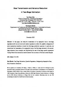
The Denovo discrete ordinates code solves a discretized form of the transport equation on a structured, rectangular mesh. The MCNP5 code uses a combinatorial geometry, in which material cells are described as volumes bounded by several possible types of surfaces (planes, cylinders, spheres, cones, etc.). A fundamental task in creating an approximate representation of the Monte Carlo model for Denovo is mapping the combinatorial geometry onto a userspecified structured grid. To illustrate the material mapping process implemented in ADVANTG, consider test problem INP12 from McKinney and Iverson (1996), shown in Fig. 3-1. This problem models an oil-well logging scenario in which an iron sonde containing two 3He detectors and a neutron source is inserted into a water-filled borehole within a limestone formation. (The geometry of 23
the problem is divided into mesh-like cells to utilize cell-based weight-window parameters from a diffusion code. The input file for this problem was created before mesh-based weight windows were available in MCNP.) For demonstration purposes, the original point source defined in the problem was changed to a volume source that fills the source cell.
Fig. 3-1. Geometry of problem INP12 with modified source.
ADVANTG performs material region mapping by ray tracing through the MCNP geometry model. The starting points of rays are randomly sampled on the exterior –x, –y, and –z faces of the mesh. Rays are then traced in the +x, +y, and +z directions to the opposite side of the mesh from the starting location. As each ray is traced, tallies record the track length through each material within each voxel of the structured grid. This process is illustrated in Fig. 3-2, which depicts two rays that started from the same external voxel face and were traced in the +x direction through the borehole region of problem INP12. In the figure, the gray dashed lines represent mesh boundaries and the blue and red crosses denote locations where the rays cross a mesh plane and an MCNP cell surface, respectively.
Once the ray tracing is completed, the track-length tallies are used to estimate the volume fractions of materials within each voxel. The material fractions are then used to generate a mixed-material specification for the Denovo calculation. Materials with volume fractions that differ by less than a tolerance value are combined to minimize the total number of mixed materials generated. The tolerance can be decreased to obtain more accurate material maps in problems where the response is sensitive to the total volume of one or more materials.
The material maps generated by ADVANTG can be displayed using the VisIt visualization software. The material map generated for problem INP12 on an 81 × 57 × 81 voxel nonuniform mesh is shown in Fig. 3-3. In the figure, two images are displayed, both of which are clipped at z = 0 to show the geometry at the center of the borehole region. In the left image, distinct material interfaces were reconstructed by VisIt before displaying the plot. (VisIt 24
applies this treatment by default.) The right image uses a “clean zones only” option, which displays voxels with mixed materials as white. No interface reconstruction is performed in either ADVANTG or Denovo, so it is important to consider the impact that material mixing will have on the discrete ordinates calculation. For this reason, examining both types of material plots is recommended.
Fig. 3-2. Ray tracing in the +x direction through problem INP12.
By default, ADVANTG will trace a minimum of ten rays from each external voxel face on the –x, –y, and –z edges of the mesh. Increasing the number of rays will produce more accurate material volume fractions and thus a more accurate deterministic calculation. (See Section 5.3.1 for a description of the ray tracer settings.) The computational time consumed by the ray tracing is proportional to the number of rays. The average cost of tracing a single ray can vary greatly between MCNP models. Ray tracing is generally more expensive in models with a large number of cells and in models that contain complicated cells (i.e., cells that are defined using the union or complement operators).
Denovo supports specularly reflective boundary conditions, but only on boundaries that are perpendicular to one of the coordinate axes. ADVANTG provides the capability to unfold reflected geometries that cannot be modeled directly by Denovo (see Section 5.3.1 for the associated input options). For example, many MCNP models of the ITER tokamak include only a sector of the reactor with reflective boundary conditions on the external azimuthal surfaces. Fig. 3-4 shows the discretized geometries generated for a 40° sector ITER model with and without the unfolding option (Ibrahim et al. 2011). Note that for certain geometries, it may be necessary to extend the boundaries of the model in order for the unfolding to work properly. In all cases, carefully inspecting the unfolded geometry in VisIt is highly recommended. 25
Fig. 3-3. Mixed material distribution of problem INP12. The left and right images were generated using the default material interface reconstruction technique and the “clean zones only” option, respectively.
Fig. 3-4. ITER 40° sector model (left) and unfolded model (right).
3.5 Source Mapping For forward, as opposed to adjoint, discrete ordinates calculations, the MCNP general fixed source (SDEF source) must be converted to a form acceptable to Denovo. ADVANTG maps the source spatial distribution by sampling source particles and tallying the voxels in which they appear. Source energy spectra are mapped onto the energy groups of the multigroup cross section library using numerical integration. ADVANTG provides two different schemes for setting the number of source samples to be drawn; the number of samples can either be set explicitly by the user or parameters can be set for ADVANTG to adaptively determine this. Because the number of samples required to 26
accurately map the source onto the spatial grid is problem dependent, ADVANTG uses the adaptive scheme by default. ADVANTG will initially sample 10,000 source particles. If fewer than ten particles were sampled in any voxel that received at least one score, an additional 20,000 particles are sampled. This process is repeated, with a doubling of the number of samples per stage, until either the target number of particles per voxel or the maximum number of samples is reached. The number of particles per stage, the target number of samples per voxel, and the maximum number of samples can all be changed from their default values. (See Section 5.3.1 for a description of the source sampling settings.) Note that a different sampling procedure, with different settings, is used to generate biased source distributions. The discretized source generated by ADVANTG can be displayed in VisIt. The source region generated for problem INP12 is shown in Fig. 3-5.
Fig. 3-5. Source regions in problem INP12.
3.6 Response (Tally) Mapping To construct adjoint source distributions for the Denovo S N calculations, ADVANTG maps surface, cell, and mesh tallies onto the user-specified spatial grid. Tally region mapping is done simultaneously with material region mapping to avoid ray-tracing through the geometry multiple times. The discretized tally regions generated by ADVANTG can be displayed in VisIt, as shown in Fig. 3-6 for problem INP12. In the figure, the tally ids correspond to the order in which they are listed in the ADVANTG input file. In this example, the near detector was listed before the far detector. ADVANTG supports cell tallies with multiple cell bins and tallies on repeated structures and lattices. Tally regions may be missed by the ray tracer if they are small relative to the mesh voxels in which they reside. If this occurs, the mesh should be refined and/or the number of rays should be increased. 27
From the perspective of the CADIS and FW-CADIS methods, all tallies have an associated energy spectrum. For example, the DE/DF cards define the response spectrum for tallies that have associated dose functions. As with forward source spectra, ADVANTG maps the response spectrum onto the multigroup structure using numerical integration. ADVANTG supports DE/DF, FM, and EM multipliers. Though MCNP allows a tally to have more than one type of multiplier, ADVANTG will select and use only a single type of multiplier. The order of precedence is: DE/DF, FM, then EM. For example, if a tally has DE/DF cards, no other multipliers are used. If no multiplier is defined, a uniform spectrum is used. For pulse-height (F8) tallies, ADVANTG uses the total cross section of the material in the tally cell as the response spectrum. This treatment has been found to be efficient for most problems involving pulse-height tallies.
Fig. 3-6. Response regions in problem INP12.
3.7 Deterministic Calculations ADVANTG obtains deterministic transport solutions by preparing inputs for and executing the Denovo 3-D, block-parallel discrete ordinates package. Denovo was selected for this purpose because it provides a powerful, robust, and efficient general deterministic transport capability. It is built around modern linear algebra solvers provided by the Trilinos library (Heroux et al. 2003) and uses the Generalized Minimum RESidual (GMRES) solver to converge within-group (scattering) iterations. This Krylov subspace solver has been shown to significantly outperform source iteration (Richardson iteration) in problems with thick scattering media. Denovo also implements several spatial discretization schemes, quadrature sets, and both analytic point-kernel and Monte Carlo-based first collision sources. For largescale problems, the transport sweeps can be performed in parallel on multiple processors. Denovo has been used to solve several problems with more than one billion spatial cells on the Jaguar supercomputer at ORNL. 28
Denovo provides multiple front ends for input. The primary and full-featured front end is implemented as a Python (scripting language) module. ADVANTG drives Denovo through this Python interface, which provides access to multiple spatial discretization schemes (stepcharacteristics, linear-discontinuous, tri-linear discontinuous, and weighted diamond difference), multiple quadrature sets (quadruple range, LDFE, Gauss-Legendre product, and level-symmetric), and the ability to perform parallel calculations.
Both group-wise and energy-integrated scalar flux solutions generated by Denovo can be displayed in VisIt. Fig. 3-7 shows the discretized material map (left) and the energy-integrated adjoint scalar flux (right) from a CADIS calculation where the far detector was the response of interest. The clip operator was used to arrange the material and flux plots next to each other. Contours were also plotted and overlaid on the pseudocolor flux plot. The near detector does not show up in the material map, because the CADIS calculation was performed on a relatively coarse mesh.
Fig. 3-7. Adjoint scalar flux in problem INP12.
It is strongly recommended that the group-wise scalar flux solution(s) be carefully studied to determine whether there are any significant non-physical or missing features (e.g., ray effects or missing source or tally regions). If necessary, the deterministic calculation(s) should be refined and the variance reduction parameters re-generated before proceeding to the Monte Carlo simulation.
29
3.8 Variance Reduction Parameter Generation ADVANTG provides two computational sequences that generate variance reduction parameters using the CADIS and FW-CADIS methods. The parameters consist of space- and energy-dependent weight-window targets and a biased source that is consistent with the weight map. The total response, 𝑅, from Eq. (2-5) and the biased source probabilities, 𝑞� , from Eq. (2-9) are estimated by sampling the original (unbiased) source distribution and scoring the importance evaluated at the source particle’s location and energy (Bevill and Mosher 2012). The total response is the average score per source particle. The biased source probabilities are averages over the bins defined by the SI cards in the MCNP input file. Once the total response is known, weight-window targets are computed according to Eq. (2-8).
ADVANTG generates and outputs biased distributions for all SB cards present in the MCNP input file, with the exception of angular and time distributions. The user’s original SB cards are used when sampling the source to compute the total response and biased probabilities. For this reason, using uniform biased probabilities is recommended to ensure that all bins are adequately sampled. In most problems, it is advantageous to partition the source bins in order to capture the spatial and energy variations of the biased source. No automatic partitioning has been implemented in ADVANTG because of the complexity of the SDEF functionality in MCNP. See Section 7 for examples of how to generate effective source biasing parameters.
When spatial source biasing is used with cell rejection, the mean weight of a source particle is no longer unity and the tally results must be adjusted by a correction factor to preserve the tally mean value. MCNP5 generates an estimate of this correction factor based on the source particles sampled during the simulation. However, it does not provide an estimate of the uncertainty in the factor, which can be significant in some cases. Because cell rejection is a useful technique, an approach for estimating the correction factor and its uncertainty has been developed and implemented in ADVANTG (Bevill and Mosher 2012). The factor directly multiplies tally results, so a conservative approach was taken to estimating its uncertainty. ADVANTG outputs the estimated correction factor and its relative error as a comment card that is included in the source biasing card output. The correction factor uncertainty can be reduced by increasing the number of samples used to estimate the biased source probabilities (see the mcnp_num_sb_samples card described in Section 5.8.1). A new, more accurate correction factor and biased source probabilities can be calculated by re-running ADVANTG at any time. No deterministic calculations will be re-run, as long as no other input changes are made.
The WWINP file created by ADVANTG contains weight-window lower bounds calculated using Eq. (2-8) with 𝑅 set to one. The value of 𝑅 normalized to a unit source strength is set as the WNORM value on the corresponding WWP card(s). (WNORM is a lower-bound multiplier; it is the seventh parameter on the WWP card.) If the SDEF card in the MCNP input file sets the initial particle weight to a value other than one, then the WNORM value should be multiplied by this modified starting weight.
30
Group-wise and energy-integrated weight-window targets can be displayed in VisIt, as shown in Fig. 3-8. The figure is analogous to Fig. 3-7, but shows the weight targets for the far detector in problem INP12. When the weights are used in an MCNP simulation, particles moving toward the detector will undergo splitting, whereas particles moving away from the detector will be subjected to roulette.
Fig. 3-8. Weight-window targets in problem INP12.
31
4. Running ADVANTG ADVANTG is executed from the command line using: $ advantg [options] input_file
Command line options are listed in Table 4-1 below. The format and content of the input file is the subject of Section 5. Table 4-1. Command line options
Option
Description
-h, --help
Print command line help and exit
--version --template [args]
Print the code version and exit
-c, --clean
Ignore existing working subdirectories. The default is to reuse existing data unless input has changed.
-f, --force-resume -g, --debug
-v, --verbose -q, --quiet
--very-quiet --silent
--log=LEVEL
Print a listing of the ADVANTG input keywords and associated descriptions. Arguments filter the keywords that are displayed. Force existing working data to be reused, even if it is outdated Write extra information to disk for debugging purposes Print all debug messages
Print only informational and warning messages Print only warning messages
Print messages only on failure
Create a log file with the given verbosity level: DEBUG, STATUS, INFO, WARNING, ERROR, or CRITICAL
The current version of ADVANTG executes only in serial mode—that is, using a single thread/core. However, ADVANTG will invoke mpirun to launch a parallel Denovo job when the product of denovo_x_blocks and denovo_y_blocks (the number of parallel domains) is greater than one. ADVANTG passes the number of domains as the argument to the mpirun –np option. In addition, if a file named machinefile is found in the problem directory (the directory in which ADVANTG was launched), then ADVANTG will add a -machinefile option to the mpirun command with the path of the file.
ADVANTG can drive parallel Denovo calculations on clusters with job submission systems. Consider a problem in which denovo_x_blocks and denovo_y_blocks are both set to 6, for a total of 36 domains. An example Portable Batch System (PBS) script is shown in Fig. 4-1 for a cluster with two hex-core processors per node. A PBS directive requests 3 nodes and 12 processes per node. Other directives set the amount of memory per process (1 GB), a 1-hour wall-clock limit, and a job name. The script sets the working directory and dumps the machinefile created by the batch system for this particular job before launching ADVANTG. When the job is started, ADVANTG begins running on a single core. When ADVANTG is ready to 33
perform a deterministic calculation, it invokes mpirun to execute a parallel Denovo calculation using 36 cores across the three nodes that were reserved for the job. #!/bin/bash #PBS -N advantg #PBS -l nodes=3:ppn=12 #PBS -l pmem=1gb #PBS -l walltime=1:00:00 cd $HOME/calcs/case1/advantg cat $PBS_NODEFILE > machinefile advantg case1.adv Fig. 4-1. Sample PBS script.
34
5. Input ADVANTG reads user input from a free-format plaintext input file. The format of the input file is described in Section 5.1 below. The sections that follow describe the various input options that ADVANTG accepts. A typical input file will contain only a small fraction of the entries described in this section. Default values are defined for most options and only a few entries are required. For MCNP models, a minimal input consists of: • • • • •
Name of an MCNP input file List of one or more tally numbers Name of a generator method (e.g., cadis or fwcadis) Lists of spatial mesh planes in the x, y, and z dimensions Name of a multigroup cross-section library
ADVANTG extracts all model-related information (e.g., geometry, materials, and sources) automatically. As a result, input files tend to consist primarily of parameters for the deterministic calculation(s).
For new users, a recommended first step is to look at the example problems in Section 7. ADVANTG inputs are shown in Figs. 7-4, 7-13, and 7-24. This section can be referred to later for more detailed information. An index of frequently used keywords is given in Appendix B.
5.1 Input File Format
ADVANTG input files are plaintext files that are organized into a series of entries or cards. Each entry begins with a case-insensitive keyword that must start within the first four columns of a line. The keyword must be followed by at least one value. Multiple values are separated by whitespace. Values can be one of the following types: • • • •
Integer literals Floating point literals Boolean literals Strings
(e.g., 0, 123, -5) (e.g., 0.5, -1.2345e+5) (e.g., true, False, 0, 1, Y, n, T, f) (e.g., gmres, "file name")
Strings containing spaces must be enclosed in double quotes (").
Entries can span multiple lines. Continuation lines are denoted by an indent of at least four columns. The length of input lines is not limited. Empty lines are ignored. Tab characters are expanded to eight spaces. With the exception of denoting a continuation line, multiple whitespace characters are treated the same as a single space.
Comments are denoted by the hash (#) character. All characters from the # character to the end of the line are ignored. Comments can start anywhere on a line and can be placed anywhere within an entry after the keyword.
35
5.2 Driver Options The following high-level options determine which components are used to carry out the computational sequence: model
name
(default: mcnp)
Type of transport problem model. One of: mcnp
MCNP5 model SWORD model
sword
method
name
(required)
Variance reduction method or type of computational sequence. One of: cadis
fwcadis dx
CADIS method (single-tally VR) FW-CADIS method (multiple-tally VR) Discretize the transport model and optionally execute deterministic calculation(s)
The dx option can be used to generate visualization output for the discretized model (see the outputs keyword below). This feature provides a means to quickly inspect the spatial mesh as well as the mapped materials, sources, and tallies, for example, as a preliminary step before proceeding to perform the transport calculations.
The dx option can also be used to execute a forward or adjoint deterministic calculation without generating variance reduction parameters. This feature is useful, for example, for performing scoping or feasibility studies or other calculations where continuousenergy Monte Carlo is not needed. outputs
name ...
(default: mcnp silo)
Type(s) of output. Any of: mcnp
silo response none
MCNP weight-window file (WWINP) and biased source cards for the cadis or fwcadis methods Silo-format visualization files Calculate, tabulate, and/or plot deterministic response estimates No specialized output
The data within Silo-format files can be visualized using the VisIt open-source, 3-D, parallel visualization package. VisIt is an extremely powerful tool for exploring meshbased data sets, and its use is highly recommended.
If the response option is selected, energy-dependent and energy-integrated responses will be calculated based on the deterministic transport solution. This option is most useful with the dx method. 36
5.3 Model Parameters 5.3.1 MCNP-Specific Parameters The options and settings described in this section apply when model is mcnp. If a different model type is selected, these settings are ignored. mcnp_input
filename
(required)
Filename of the MCNP5 input file. Enclose the filename in double quotes if it contains spaces. mcnp_tallies
int ...
MCNP tally number(s) for which to generate variance reduction parameters and/or to use in forming adjoint sources. This keyword is required if a deterministic adjoint calculation will be performed. mcnp_material_names
int name ...
Names of MCNP materials for output purposes, listed as pairs of MCNP m card numbers and name strings. If the silo output option is selected, the material names will be written to the Silo file and appear in VisIt. By default, material 0 is named void. Example:
mcnp_material_names
mcnp_input_template
1 10 11
Air He-3 “Stainless steel”
filename
For CADIS or FW-CADIS calculations, the filename of an alternate MCNP5 input file to use as a basis for generating a new MCNP input with biased source (SB) and weightwindow parameter (WWP) cards. The template file is not modified. By default, mcnp_input is used. The new input file, named inp, is written to the output/ directory. This feature may be useful when it is necessary to modify the MCNP input just for the purpose of running ADVANTG (e.g., see Sections 8.1 and 8.2).
37
The following parameters control the number of samples drawn from the MCNP SDEF source when mapping it onto the spatial mesh. Note that these parameters do not affect the calculation of biased source distributions (instead, see the mcnp_num_sb_samples keyword in Section 5.8.1). mcnp_num_source_samples
int > 0
(default: 10000)
Number of times to initially sample the SDEF source. mcnp_min_source_voxel_samples
int > 0
(default: 10)
Target minimum number of samples to obtain in each mesh voxel. If the target is not reached after mcnp_num_source_samples, up to mcnp_max_source_samples will be drawn in an attempt to reach the target. A warning message is printed if the target is not reached. mcnp_max_source_samples
int
(default: -16)
If positive, the maximum number of times to sample the SDEF source. If negative, the limit is calculated as: |mcnp_max_source_samples| × mcnp_num_source_samples
If zero, no upper limit is defined. Particles will be sampled until the mcnp_min_source_voxel_samples criterion is satisfied (use with caution).
The following parameters control the number and direction of rays traced through the MCNP geometry to map materials and tally regions onto the spatial mesh. mcnp_min_rays_per_face
int > 0
(default: 10)
Minimum number of rays to trace through each voxel face in each trace direction. mcnp_ray_directions
axis ...
(default: x y z)
Directions in which to trace rays through the MCNP geometry model. Rays are traced parallel to the spatial axes and in the positive direction. Any combination of x, y, and/or z can be selected. mcnp_num_rays
int > 0
(default: 1)
Nominal total number of rays.
The nominal number of rays to be traced through each voxel face is calculated in proportion to the area of the face. The per-face minimum is then applied so that the actual number of rays is the greater of the nominal number and the mcnp_min_rays_per_face setting (10 rays, by default). 38
By default, the mcnp_min_rays_per_face setting determines the total number of rays that are actually sampled. The mcnp_num_rays setting is provided because it can be useful in problems where the spatial mesh voxels vary greatly in size. mcnp_lost_rays
int
(default: 10)
Maximum number of lost rays allowed while mapping material and tally regions onto the spatial mesh. An error message is printed if the limit is reached. mcnp_mix_tolerance
real >= 0.0
(default: 0.01)
Tolerance for combining mixed materials. Materials with component volume fractions that differ by less than or equal to this amount will be combined to minimize the total number of mixed materials generated. Higher numbers reduce the amount of memory needed to store material mixtures. Lower numbers provide more accurate per-voxel discretized material compositions.
For example, if voxels A, B, and C contain 70, 90, and 91% steel by volume, respectively, and 30, 10, and 9% air, then by default voxels B and C will contain the same mixed material. Voxel A will contain a different mixture. The following parameters control the unfolding options that can be used if the MCNP5 model has reflecting boundaries. mcnp_unfolding_origin
real(3)
Specifies the x, y, and z coordinates of a reference point inside a reflected MCNP geometry that is to be unfolded for the Denovo deterministic calculations. Avoid placing the reference point near external surfaces. Note that the rays used to perform the unfolding are terminated when they reach a cell of zero importance. For certain geometries, it may be necessary to extend the model with one or more voided cells that have non-zero importance in order for the unfolding to work properly. In all cases, careful inspection of the unfolded geometry in VisIt is highly recommended. mcnp_unfolding_safe
bool
(default: False)
If True, activates a “safe” ray tracing mode for the unfolding process. This safe mode is slower than the default mode, but the probability of generating lost rays is lower. Use the safe mode only if you run into issues with lost rays when using the default mode.
39
5.3.2 SWORD-Specific Parameters The options and settings described in this section apply when model is set to sword. If a different model type is selected, these settings are ignored. sword_input
filename
(required)
Filename of the .sword file. Enclose the filename in double quotes if it contains spaces. sword_mix_tolerance
real
(default: 0.01)
Tolerance for combining mixed materials (analogous to mcnp_mix_tolerance). Materials with component volume fractions that differ by less than or equal to this amount will be combined to minimize the total number of mixed materials generated. Higher numbers reduce the amount of memory needed to store material mixtures. Lower numbers provide more accurate per-cell discretized material compositions. sword_small_sources
bool
(default: True)
If True, single-voxel sources are approximated as a point source of equivalent strength to activate the first-collision source treatment in Denovo. Generally, this substitution yields more accurate deterministic results. sword_sampling
name
(default: subcell)
Sampling algorithm to be used for discretizing the SWORD geometry. One of: subcell res
sword_subcell sword_subcell_x sword_subcell_y sword_subcell_z
Specify the number of samples per cell Specify a minimum sampling resolution
int “ “ “
(default: 2)
When sword_sampling is subcell, the sword_subcell keyword sets the number of point samples per interval in each spatial dimension. The dimension-specific keywords can be used to override this setting for a particular dimension.
For example, when sword_subcell is 1, material compositions are based on the material found at the center of each voxel. When the value is 2, eight samples per voxel are used to generate a mixed-material description of the contents of the voxel.
40
sword_resolution
float
When sword_sampling is res, sets the length, in cm, of the desired point sampling interval for each spatial dimension. For example, if sword_resolution is set to 2.0, then in a voxel with dimensions 10 × 6 × 4 cm, 5 point samples will be taken along the x dimension, 3 along y, and 2 along z, for a total of 30 samples within the voxel.
5.4 Method Options
No CADIS-specific input parameters are currently defined.
5.4.1 FW-CADIS-Specific Parameters fwcadis_spatial_treatment
name
(default: pathlength)
Spatial treatment used when constructing the FW-CADIS adjoint source. One of: pathlength global
Use path-length weighting Use global weighting
The pathlength treatment is recommended for problems with multiple cell, surface, and/or point detector tallies. The global treatment is recommended for mesh tallies. See Sections 2.3.1 and 2.3.2 for more details. fwcadis_response_weighting
bool
(default: True)
If True, construct the adjoint source to accelerate an energy-integrated response (e.g., dose or total flux). If False, generate parameters with the objective of obtaining relatively uniform uncertainties across all energy groups. See Sections 2.3.3 and 2.3.4 for more details.
Note that turning off response weighting generally increases the time per history in the Monte Carlo simulation, especially if the group-wise flux in the region of interest varies over many orders of magnitude. fwcadis_min_response fwcadis_max_response
real >= 0. “
(default: 0) (default: infinite)
Lower and upper energy-integrated response thresholds for including voxels when constructing the FW-CADIS adjoint source with the global spatial treatment. By default, no threshold is used.
This feature can be useful, for example, when estimating dose rate maps. In practical applications, there is generally no interest in dose rates that fall below a certain level. By excluding the adjoint source from the region outside of a particular dose rate contour, a more efficient Monte Carlo simulation is obtained. 41
Note that the locations of the upper and lower thresholds are calculated based on the deterministic solution, which might not be highly accurate. It is therefore recommended to set the lower/upper threshold somewhat lower/higher than the actual contour of interest (e.g., by one or two orders of magnitude). To ensure that the thresholds are properly chosen, the responses calculated using the deterministic and MCNP models should be compared. If the difference between these responses is larger than the margin applied to the threshold values, those values should be adjusted and the ADVANTG calculation should be re-run.
5.4.2 DX-Specific Parameters
The dx option provides the means to discretize the model and optionally execute deterministic calculations without generating variance reduction parameters. The options described below control which deterministic calculations are performed, if any. dx_adjoint dx_forward
bool “
(default: False) “
If True, executes a deterministic calculation in the specified transport mode. By default, no deterministic calculations are executed; the model is discretized, and the quality of the result can be visualized using the appropriate output options (see Section 5.8.2).
5.5 Spatial Mesh
The following settings are used to construct a 3-D rectangular spatial mesh as the product of 1-D meshes in the x, y, and z dimensions. The mesh of the weight-window map is the same as that used in the deterministic calculations. mesh_refinement
name
(default: mcnp)
Technique for refining the mesh. One of: mcnp
uniform
Use the mesh_x_ints, mesh_y_ints, and mesh_z_ints keywords Use the mesh_max_width and mesh_min_width keywords
The mcnp option uniformly subdivides each mesh interval. The uniform option adds and/or removes voxel edges in an attempt to generate nearly uniform widths across each dimension.
42
mesh_x mesh_y mesh_z
real ... “ “
(required) “ “
Coordinates of mesh voxel edges in the x, y, and z dimensions, in cm. At least two edges per dimension are required. The edge coordinates must be listed in increasing order. The mesh can be refined using one of two approaches described with the
mesh_refinement keyword. By default, the mesh intervals are not subdivided further and the mesh_x, mesh_y, and mesh_z cards define the final mesh. mesh_x_ints mesh_y_ints mesh_z_ints
int > 0 ... “ “
(default: 1 subdivision per mesh interval) “ “
The number of uniform subdivisions in each mesh interval when mesh_refinement is mcnp. Ignored if mesh_refinement is not mcnp. By default, the original mesh intervals are not subdivided further. The number of entries must be one less than for mesh_x, mesh_y, or mesh_z. Example:
mesh_x 0 mesh_x_ints
10 2
20 4
These cards define a spatial grid in the x-dimension that has voxel edges at the coordinates: 0, 5, 10, 12.5, 15, 17.5, and 20 cm. mesh_max_width mesh_x_max_width mesh_y_max_width mesh_z_max_width
real > 0. “ “ “
Maximum distance between voxel edges, in cm, when mesh_refinement is uniform. Required if mesh_refinement is uniform and ignored otherwise. The mesh_max_width keyword sets the default maximum width for all dimensions. The dimension-specific keywords can be used to override this setting for a particular dimension. mesh_min_width mesh_x_min_width mesh_y_min_width mesh_z_min_width
real >= 0. “ “ “
(default: 0.0) “ “ “
Minimum distance between voxel edges, in cm, when mesh_refinement is uniform. Ignored if mesh_refinement is not uniform. The mesh_min_width keyword sets the default minimum width for all dimensions. The dimension-specific keywords can be used to override this setting for a particular dimension.
By default, the minimum voxel width is zero, and none of the grid points specified on the mesh_x, mesh_y, or mesh_z cards will be removed. 43
Example:
mesh_x -10 -5.5 mesh_min_width 0.75 mesh_max_width 2
0
0.25
5.5
10
These input cards will generate an x-dimension spatial grid that has voxel edges at: -10, -8.5, -7, -5.5, -3.67, -1.83, 0, 1.83, 3.67, 5.5, 7.0, 8.5, and 10 cm.
Note that the original edge at 0.25 cm has been removed because mesh_min_width is 0.75 cm. This can be avoided by setting the minimum width to 0.25 cm or smaller.
5.6 Multigroup Library Options
ADVANTG reads multigroup cross section data from ANISN-format libraries. The options described in this section can be used to select a cross section library, set the upscatter treatment, and define mappings of ZAIDs to cross section tables. anisn_library
name
(required)
Name of the ANISN-format cross section library (see Section 3.2 for a list of library names). The search path defined in the configuration file is searched to locate the library and associated metadata files. anisn_upscatter
bool
(default: False)
If False, then treat upscatter as self-scatter and avoid costly upscatter iterations in the Denovo calculation(s). If the accuracy of thermal neutron fluxes is important, then consider setting anisn_upscatter to True. This option has no impact on photon-only problems. anisn_zaid_map
int > 0 ...
Additional ZAID and ANISN table id pairs to use when mapping the MCNP material compositions to multigroup materials for the deterministic calculation. An arbitrary number of pairs can be given. Entries on this card add to or override the mappings defined in the .zaid file associated with the selected ANISN library.
44
5.7 Solver Options The Denovo discrete ordinates solver provides a variety of options and settings. For generating variance reduction parameters, typically only a fraction of these settings are used or modified. The most frequently used parameters are: • denovo_quadrature and associated options, which select and configure the S N angular approximation, • denovo_pn_order, which determines the degree of scattering anisotropy modeled, and • denovo_x_blocks and denovo_y_blocks, which determine the parallel spatial decomposition (if Denovo was built with an MPI library). The amount of memory consumed by the Denovo solver state (i.e., by the discrete ordinates solution in memory) is state size = 𝑁𝑐 �𝑁𝑔 + 𝑁𝐾 �(𝐿 + 1)2 𝑁𝑢 ∙ 8 bytes,
(5-1)
where 𝑁𝑐 is the number of mesh voxels, 𝑁𝑔 is the number of solved energy groups, 𝑁𝐾 is the number of Krylov vectors (default is 20), and 𝐿 is the scattering expansion order. 𝑁𝑢 is the number of unknowns per voxel and is determined by the spatial discretization scheme (see below). The factor of eight is because the solver state is stored in double precision. Firstcollision and FW-CADIS adjoint sources may consume significant amounts of additional memory. In addition, a small overhead (for communication buffers, local-to-global maps, etc.) is added for each process when Denovo is executed in parallel. Thus, Eq. (5-1) represents a lower limit, not an upper bound. For cluster jobs, the number of nodes and/or the number of cores per node should be selected so that the memory usage per node does not exceed the available memory (with an allowance for the operating system and any other running jobs). The following options and settings control the spatial discretization and parallel spatial decomposition: denovo_discretization
name
(default: sc)
Spatial discretization. One of: ld sc
tld twd wdd wdd_ff
Linear discontinuous Step characteristics Tri-linear discontinuous Theta-weighted diamond Diamond difference Diamond difference with negative flux fixup
𝑁𝑢 4 1 8 1 1 1
The step-characteristics discretization scheme is robust with regard to mesh size and voxel aspect ratios and always produces positive fluxes given positive sources. It has first-order accuracy (i.e., the discretization error decreases linearly with mesh size in the asymptotic limit) and requires storage of only one unknown per voxel in memory. Because of its robustness, positivity, and low memory requirements, it is the default scheme in ADVANTG. Note that the step-characteristics method will tend to overestimate the fluxes deep within an attenuating material. 45
The linear and tri-linear discontinuous (LD and TLD) schemes have second-order accuracy, but do not ensure positivity. The LD and TLD methods require storage of four and eight unknowns per voxel, respectively, and also incur a similar increase in run time. These discretization schemes tend to give very accurate results on well-refined meshes but can break down on coarser grids. The LD scheme tends to be rather sensitive to the aspect ratio of the mesh voxels. The TLD scheme is more robust than LD, but incurs a significant cost relative to step characteristics.
The diamond difference and theta-weighted diamond techniques have a long history. The weighting helps to dampen, but does not entirely eliminate, the oscillations exhibited by diamond difference solutions in 3-D problems. It also reduces the order of accuracy to somewhere between first and second order. Because the step characteristics scheme provides significantly better solutions in most problems, the use of the diamond difference technique is generally discouraged. denovo_x_blocks denovo_y_blocks denovo_z_blocks
int > 0 “ “
(default: 1) “ “
The number of spatial domain partitions in the x and y dimensions, and the number of pipelining blocks in the z dimension.
The Koch-Baker-Alcouffe 3-D parallel sweep algorithm is implemented in Denovo on a domain that is decomposed into x-y blocks. Each parallel core is assigned a single x-y block. So for example, with denovo_x_blocks and denovo_y_blocks both set to 2, a parallel calculation across four cores is performed. The number of blocks in each dimension should be chosen in proportion to the number of mesh intervals.
The x-y blocks can be divided into multiple blocks in the z dimension. The z dimension blocks do not affect the domain decomposition (or the number of cores used) but determine the frequency at which fluxes are communicated between neighboring domains. This setting can impact performance in problems that have a large number of intervals in the z dimension. By default, a single-core calculation is performed with no domain decomposition. Note that Denovo must be built with an MPI library (OpenMPI or MPICH) in order to execute parallel calculations.
The following options control the partitioning of the energy groups across processors: denovo_energy_sets
int > 0
(default: 1)
The number of parallel partitions in energy.
The parallel performance of the solver scales well with the number of spatial domain blocks. At some point, however, the domain blocks are small enough that communication overhead reduces efficiency. Energy partitioning provides a means to maintain solver efficiency across a larger number of cores. The number of executing 46
cores is the product of the number of x-y domain blocks and the number of energy sets. This feature is generally needed only in massively parallel S N calculations. denovo_partition_upscatter
bool
(default: False)
If True, partition just the upscatter groups. This option is only valid when more than one energy set is used and when anisn_upscatter is True (see Section 5.6). The following options and settings control the S N angular quadrature: denovo_quadrature
name
(default: qr)
Type of quadrature set. One of: glproduct ldfe
levelsym qr userdefined
Gauss-Legendre product Linear-discontinuous finite element (triangular) Level-symmetric (triangular) Quadruple range (product or triangular) User-defined set
Denovo provides several types of angular quadratures, which fall into two basic classes: triangular and product. Triangular quadrature sets are characterized by an integer order (see the denovo_quad_order or denovo_ldfe_order keywords). Product quadratures are determined by the number of azimuthal and polar angles per octant (see the denovo_quad_num_azi and denovo_quad_num_polar keywords). Triangular quadrature sets are generally rotationally symmetric, whereas product quadrature sets are generally not. However, product quadratures provide the flexibility to vary the number of azimuthal and polar angles independently, which can be more efficient in some types of transport problems.
Note that the run time of the S N calculations scales nearly linearly with the number of quadrature angles (all else being equal). For triangular quadratures, the number of angles does not increase linearly with the order (see below). Memory usage is independent from the number of angles, because only the (𝐿 + 1)2 angular moments are retained in memory.
Gauss-Legendre (GL) product quadratures are formed as the Cartesian product of a set of uniformly distributed azimuthal angles and a 1-D Gauss-Legendre quadrature in the polar angle.
Linear-discontinuous finite element (LDFE) quadratures (Jarrell 2010) are based on an approach that approximates the angular flux as 𝜓 ≈ 𝑐1 + 𝑐2 𝜇 + 𝑐3 𝜂 + 𝑐4 𝜉, where 𝜇, 𝜂, and 𝜉 are the direction cosines with respect to the coordinate axes. The quadrature is determined by requiring that the integration of the basis functions equals the surface area of the unit sphere. The LDFE sets have positive weights and are rotationally symmetric about all three axes. There are 4(𝑁+1) angles per octant, where 𝑁 is the order. Unlike level-symmetric quadratures, the LDFE order can be even or odd. The maximum LDFE order in Denovo is seven. 47
Level-symmetric quadratures have a long history with the S N method. They are rotationally-symmetric quadratures that have positive weights up to S 20 . In 3-D, there are 𝑁(𝑁 + 2)/8 angles per octant, where 𝑁 is the order. The maximum order supported by Denovo is 24. The order must be an even number.
Quadruple range (QR) product quadratures (Abu-Shumays 2001) exactly integrate maximal-order products of sines and cosines of the polar and azimuthal angles. The maximum number of azimuthal and polar angles per octant for QR quadratures in Denovo is 37 and 16, respectively. The QR product quadratures perform well across a broad range of transport problems and tend to exhibit far less ray effects than levelsymmetric quadratures. For these reasons, the QR product set with four azimuthal and four polar angles per octant is the default quadrature used by ADVANTG. This set is often sufficient for generating variance reduction parameters for neutron-only problems. For photon-only problems or Denovo-only calculations, a more refined quadrature set is generally recommended. Denovo also implements the QR quadrature as a triangular type quadrature that contains the same number of angles as a level-symmetric quadrature set of the same order. However, the triangular QR quadrature is not rotationally symmetric. The maximum order is 32. For non-symmetric quadratures (GL and QR), the default polar axis is the z-axis. A different polar axis can be selected using the denovo_quad_polar_axis keyword. Denovo also provides the facility to read in user-provided quadratures. See the denovo_quad_file keyword below. denovo_quad_order denovo_ldfe_order
even int > 1 int > 0
(default: 10) (default: 1)
Triangular quadrature orders. The denovo_quad_order keyword sets the order for level-symmetric and triangular QR sets. The maximum orders implemented in Denovo for the level-symmetric, QR, and LDFE quadratures are 24, 32, and 7, respectively. Note that for orders greater than 20, the level-symmetric quadratures will contain some negative ordinate weights. denovo_quad_num_azi denovo_quad_num_polar
int > 0 “
(default: 4) “
Number of azimuthal and polar directions per octant for product quadrature sets. The maximum number of azimuthal and polar angles per octant for QR quadratures is 37 and 16, respectively. There are no such limits for the GL product quadrature.
48
denovo_quad_polar_axis
axis ...
(default: z)
Polar axis for non-symmetric quadrature sets. Must be one of: x, y, or z. denovo_quad_file
filename
Filename of a user-provided quadrature file. Ignored unless denovo_quadrature is userdefined.
The quadrature file is a free-format plaintext file. The direction cosines and weight of each quadrature direction are listed on a single line as: 𝜇𝑛 𝜂𝑛 𝜉𝑛 𝑤𝑛 . The direction cosines must be normalized so that 𝜇2 + 𝜂 2 + 𝜉 2 is within 1 ± 10−6. The weights must be strictly greater than zero. Lines with a hash character (#) in the first column are ignored. The following options and settings control the treatment of scattering. If anisn_upscatter is False (the default), no upscatter iterations are performed. Upscatter iterations are performed if anisn_upscatter is True and the multigroup library contains upscatter data. denovo_pn_order
int >= 0
(default: 3)
Order of the Legendre scattering-angle expansion. Denovo supports scattering expansions up to 11th order. Most multigroup cross section libraries have scattering data up to 5th or 7th order.
The memory consumed by Denovo scales as (L + 1)2, where L is the scattering order. Thus, a P 3 calculation consumes four times more memory than a P 1 calculation.
Generally, a relatively high expansion order (P 3 and above) is recommended for photon and coupled neutron-photon calculations. A lower order can often lead to a negative scattering source (caused by truncation error); this can produce negative fluxes, even with the step characteristic differencing scheme. Negative fluxes are still possible with a higher-order expansion; however, the magnitudes of any negative scattering sources are generally much lower. It is possible to enforce a positive scattering source (see denovo_transport_correction) at the expense of accuracy.
49
denovo_transport_correction
Transport correction. One of: cesaro
name
(default: diagonal)
Cesaro positive-preserving 𝑔𝑔
𝜎�𝑔 = 𝜎𝑔 − 𝜎𝑠 𝐿+1 𝑔𝑔 𝑔𝑔 𝑔𝑔 𝜎�𝑠 𝑙 = 𝜎𝑠 𝑙 − 𝜎𝑠 𝐿+1 , 𝑙 = 0, … , 𝐿
diagonal none
No transport correction
The diagonal transport correction should provide accurate results for most problems. The Cesaro correction ensures a positive scattering source, but at the expense of accuracy. It can be used if denovo_pn_order is at least 2. Denovo contains two embedded first-collision source capabilities: an analytic point-kernel treatment and a Monte Carlo implementation for distributed sources. The Monte Carlo implementation traces rays from randomly sampled starting points in randomly sampled directions. It can only be used with sources that have a single energy spectrum.
Point sources on the MCNP SDEF cards are handled with the analytic first-collision source. The Monte Carlo first-collision source treatment must be explicitly activated for distributed sources using the following options and settings: denovo_mc_first_collision
bool
(default: False)
If True, enables the Monte Carlo first collision source for distributed sources. By default, no first-collision source treatment is applied to distributed sources. denovo_mc_num_particles
int > 0
(default: 10000)
Number of particles to simulate with the Monte Carlo first collision treatment. The following options and settings control the within-group and upscatter solvers: denovo_solver
name
(default: gmres)
Within-group solver. One of: gmres si
Restarted GMRES solver Source (Richardson) iteration
The GMRES solver generally converges more quickly and is able to converge to tighter tolerances than source iteration, especially for problems with thick scattering media.
50
denovo_multigroup_solver
name
(default: gauss_seidel)
Upscatter solver. One of:
gauss_seidel Gauss-Seidel solver gmres Restarted GMRES solver
This option is ignored if anisn_upscatter is False. The GMRES upscatter solver will generally converge more rapidly than Gauss-Seidel iterations. However, the GMRES option is not currently compatible with either first-collision source implementation. denovo_preconditioner
name
(default: none)
Preconditioner for the within-group solver. One of: dsa
Diffusion synthetic acceleration No preconditioner
none
denovo_two_grid
bool
(default: False)
If True and if anisn_upscatter is True, enables two-grid upscatter acceleration. denovo_krylov_space
int > 0
(default: 20)
Maximum number of Krylov vectors to store for the GMRES within-group solver.
Reducing the number of vectors reduces the memory consumed by Denovo, particularly in problems with a relatively small number of solved energy groups (e.g., as in photononly calculations). Setting the number of vectors too low can increase the number of within-group iterations needed to reach the convergence criterion or prevent convergence altogether. Increasing the number of Krylov vectors beyond the default value typically has no benefit. denovo_max_iterations
int > 0
(default: 100)
Maximum number of within-group iterations.
The GMRES solver will generally converge well before the default upper limit is reached, even in problems with thick scattering materials. Nonetheless, the number of actual iterations per group should be studied to ensure that all within-group solves were converged.
51
denovo_tolerance
real > 0.
(default: 0.001)
Convergence criterion for the within-group iterations.
The convergence measure used by Denovo is the 𝐿2 norm of the residual vector for the GMRES solver and the 𝐿∞ norm for the source iteration solver. These measures are not equivalent to the pointwise relative flux difference that is used in some other transport codes. The criterion of 10-3 has generally been found to be sufficient for the purpose of generating variance reduction parameters. For Denovo-only calculations, it is recommend to set this limit to 10-5 or lower. denovo_upscatter_tolerance
real > 0.
(default: 0.01)
If anisn_upscatter is True, the convergence tolerance for the upscatter source. denovo_upscatter_inner_iterations
int > 0
(default: 10)
If anisn_upscatter is True, the maximum number of iterations for each within-group solve in the upscatter iteration. denovo_upscatter_inner_tolerance
real > 0.
(default: 0.01)
If anisn_upscatter is True, the tolerance for each within-group solve in the upscattering iteration. denovo_first_group denovo_last_group
int >= 0 int >= 0
(default: 0)
The first and last energy groups to be solved. Note that in Denovo and ADVANTG, energy groups are indexed from zero rather than one. See Appendix A for listings of the group boundaries of the cross section libraries that are distributed with ADVANTG. By default, the last group is the lowest energy neutron group in neutron-only problems and the lowest energy photon group in photon-only and coupled neutron-photon problems. The following option(s) control the output of Denovo: denovo_verbose
bool
(default: True)
If True, extra solver output (debug information, convergence information, and input configuration) is written to the stdout file when Denovo is executed.
52
5.8 Output Options 5.8.1 MCNP-Specific Parameters mcnp_mxspln
int >= 2
(default: 100)
Maximum number of weight-window splits per event. This parameter is written as the MXSPLN entry of the WWP card(s) in the generated MCNP input file. mcnp_num_sb_samples
int > 0
(default: 10)
Number of times to sample each combination of SDEF source distribution bins when generating the source biasing parameters and estimating the mean source weight. mcnp_ww_ratio
real >= 2.0
(default: 5.0)
Ratio of the upper to lower weight-window bounds. This parameter is written as the WUPN entry of the WWP card(s) in the generated MCNP input file.
5.8.2 Silo-Specific Parameters silo_response_ids silo_source_ids
bool “
(default: True) “
If True, writes maps of individual response or source identifiers to the Silo output file. silo_source_strength
bool
(default: True)
If True, writes the distribution of the volume-averaged, energy-integrated source strengths to the Silo output file. silo_ww
bool
(default: False)
If True, writes an expression for the weight-window targets to the Silo output file. The expression has a negligible effect on the size of the Silo file. This option is only valid when an adjoint solution has been calculated.
53
silo_edit_reactions
int name ...
Specifies one or more edit fields to be calculated and written to the Silo output file, listed as pairs of edit reaction numbers and name strings. Edit reaction cross sections (or dose functions, fission spectra, etc.) are located in the ANISN cross section table in positions 1 to (IHT – 1), where IHT is the location of the total cross section. The number of edits available and the contents of the edits are library-specific.
Note that Silo field names can contain only alphanumeric characters and underscores (_).
Example:
silo_edit_reactions
1
nu_sigma_f
54
6. Output The primary output from ADVANTG is a WWINP file containing space- and energydependent weight-window lower bounds and the user’s MCNP input file extended with biased source distributions and weight-window control parameters. Both files are written in a format compatible with unmodified versions of MCNP. ADVANTG also outputs status, warning, and error messages (if any) to the terminal window. Status messages are intended to indicate the progress of the computational sequence. Warning and error messages indicate potential or actual problems in inputs or computational results.
ADVANTG has the capability to write materials, scalar flux fields, sources, and responses in Silo format. Silo is an open-source library that provides an interface for reading and writing mesh-based data fields to a binary file, or to multiple files in parallel. The data in Silo files can be visualized using the VisIt visualization software. This functionality provides a means for the user to review the discretized model and flux estimates generated by Denovo. The user should carefully study this information to determine if obvious non-physical features are present in important parts of the solution. If so, then input parameters must be modified to produce a more accurate deterministic calculation.
When ADVANTG is executed, it creates several directories below the current working directory. A listing of the directories that can be created, depending on the calculation sequence, is shown in Table 6-1. In these directories, ADVANTG stores nearly all of the data that it generates, as well as input and output files for the codes that it executes. Much of this information, with the exception of large data arrays, is in a human-readable format that can be reviewed and inspected in case any problems arise. By default, ADVANTG will reuse as much of this data as possible if it is executed again. For example, if a tally is added to an FW-CADIS calculation, then the source mapping and forward Denovo calculation can be re-used and will not be re-executed.
55
Table 6-1. Problem sub-directories
Directory adj_solution/ fwd_solution/ fwcadis_adj_solution/ model/
output/
Description Denovo working directory for adjoint discrete ordinates calculations with the cadis and dx methods.
Denovo working directory for forward discrete ordinates calculations with the fwcadis and dx methods. Denovo working directory for adjoint discrete ordinates calculations with the fwcadis method.
Working directory for model discretization tasks. For MCNP models, MCNP is executed in this directory to create the runtpe file from which ADVANTG extracts model information. Output directory. Contains the WWINP file and modified MCNP input file if variance reduction parameters were calculated. If Silo output was requested (the default), contains the fields.silo file that can be opened in VisIt. Also contains the status.log file, which records all status, warning, and error messages.
56
7. Examples This section presents three example problems that demonstrate the use of ADVANTG to generate variance reduction parameters for continuous-energy MCNP5 simulations. The first example uses the CADIS method to accelerate a point detector tally. The second and third examples use the FW-CADIS method to obtain relatively uniform statistical uncertainties across the energy bins of a pulse-height tally and the voxels of a mesh tally, respectively. MCNP and ADVANTG input files for all three example problems can be found in the examples/ directory of the ADVANTG distribution.
7.1 Ueki Shielding Experiments 7.1.1 Background
Ueki et al. (1992) describe a series of experimental measurements that were conducted to investigate the neutron shielding properties of several materials. A schematic of the experiment is shown in Fig. 7-1 (reproduced from Ueki et al., Fig. 2). In the figure, all dimensions are listed in centimeters (cm). A 252Cf neutron source with a strength of 4.05 × 10⁷ n/s was placed at the center of a 50 × 50 × 50 cm block of paraffin with a 45° cone-shaped opening at the front. A neutron dosimeter, providing dose-equivalent rates, was placed behind slabs of shielding material. The shielding material and thickness T were varied over the course of the experiment.
The measured results are shown in Fig. 7-2 (Ueki et al., Fig. 3). The results are reported in terms of an attenuation factor, defined as attenuation factor =
𝑑𝑜𝑠𝑒| 𝑇 . 𝑑𝑜𝑠𝑒| 𝑇=0
(7-1)
No uncertainties in the measured results were reported. For the KRAFTON N2 shielding material, the authors compared measured attenuation factors to results from MCNP2B simulations. Ratios of calculated to experimentally measured results (C/E ratios) ranged from 0.84 to 1.04. Unfortunately, tabulated results were reported only for the KRAFTON material. Results for the other materials were reported in the lin-log plot shown in Fig. 7-2.
7.1.2 Objective
Use ADVANTG to accelerate continuous-energy MCNP simulations of the graphite shielding experiments performed by Ueki. Estimate neutron dose attenuation factors for shield thicknesses of T = 0, 2, 5, 10, 15, 20, 25, 30, and 35 cm. Compare the results obtained with and without the ADVANTG-generated weight-window and source biasing parameters. Determine if any statistically significant difference exists between the sets of results.
57
Fig. 7-1. Schematic arrangement of source, shields, and detector (Fig. 2 from Ueki et al.).
Fig. 7-2. Measured dose attenuation factors (Fig. 3 from Ueki et al.). 58
7.1.3 MCNP Model and Results MCNP input files were constructed based on the dimensions shown in Fig. 7-1. Continuous energy ENDF/B-VII.0 cross sections were used for the paraffin and graphite materials, which were modeled at densities of 0.93 and 1.7 g/cm3, respectively. All other regions were modeled as void. The poly.10t and grph.10t S(α,β) tables were used for paraffin and graphite, respectively.
A point neutron source was placed at the center of the paraffin block, as shown in Fig. 7-3. An offset of 0.001 cm was used, so as to avoid placing the source directly on a surface. The source spectrum was modeled as a Watt fission distribution. The neutron dosimeter was idealized as a point detector tally with associated ANSI/ANS-6.1.1 1977 flux-to-dose-rate conversion factors on DE/DF cards. The point detector was placed 20 cm behind the back of the shield. To illustrate that the ADVANTG variance reduction parameters are effective at increasing the number of particle tracks in the vicinity of the detector, an F4 tally was defined over a 5 × 5 × 5 cm cube surrounding the detector point.
MCNP simulations were performed on a hex-core Intel Xeon X5690 processor running at 3.47 GHz. A run-time limit of 6 min per case was used. All simulations were performed using only a single core. Tally results for the nine different shield thicknesses are summarized in Table 7-1. All point detector tallies had relative uncertainties of less than 2% and large figures of merit. However, the F4 tally results exhibit much larger uncertainties. This is expected, because the volume of the tally cell is small. Though variance reduction parameters are not particularly needed for these simulations, the well-converged point detector results provide a good basis of comparison for the ADVANTG results that will be generated later.
Source
Detector
Fig. 7-3. MCNP model of Ueki experiment for the T = 35 cm case.
59
Attenuation factors were calculated based on Eq. (7-1) and are shown in Table 7-2. The table also lists C/E ratios based on experimental values obtained by reading the plot shown in Fig. 7-2. Consequently, the experimental values contain both measurement and reporting uncertainty. For the point detector tally, the C/E ratios range from 1.01 to 1.07, which is roughly comparable to the C/E ratios reported by the authors for the KRAFTON material. Table 7-1. MCNP5 dose rate results for the Ueki problem
Graphite thickness (cm) 0
F4 tally Dose rate (µSv/h)
F5 tally FOM
Dose rate (µSv/h)
FOM
454 ±
8%
25
505 ± 0.1%
115741
2
449 ±
8%
26
442 ± 0.3%
17343
5
359 ±
9%
20
372 ± 0.5%
7234
10
245 ± 10%
16
269 ± 0.7%
3604
15
182 ± 12%
11
193 ± 0.9%
2202
20
133 ± 14%
8
132 ± 1.0%
1483
25
89 ± 17%
6
89 ± 1.3%
986
30
56 ± 20%
4
59 ± 1.6%
668
35
45 ± 23%
3
40 ± 1.9%
467
Table 7-2. MCNP5 attenuation factor results for the Ueki problem
Graphite thickness (cm) 2
Attenuation factor
C/E
Attenuation factor
C/E
0.989 ± 11%
1.19
0.876 ± 0.3%
1.06
5
0.791 ± 12%
1.10
0.737 ± 0.5%
1.02
10
0.539 ± 13%
1.02
0.533 ± 0.7%
1.01
15
0.401 ± 15%
1.10
0.382 ± 0.9%
1.05
20
0.292 ± 16%
1.15
0.261 ± 1.1%
1.03
25
0.196 ± 19%
1.14
0.177 ± 1.3%
1.03
30
0.123 ± 21%
1.09
0.116 ± 1.6%
1.03
35
0.098 ± 25%
1.32
0.079 ± 1.9%
1.07
F4 tally
F5 tally
60
7.1.4 ADVANTG Calculations ADVANTG input files were created to generate variance reduction parameters using the CADIS method. The input for the T = 35 cm case is shown in Fig. 7-4 below. The point detector (tally 5) was defined as the response of interest for the CADIS calculation. ADVANTG defines a point adjoint source at the location of the point detector. This is advantageous, because all point sources are handled with the first-collision treatment in Denovo. This approach greatly reduces ray effects that would otherwise result from small volume sources in non-scattering media. Because the point detector lies at the center of the F4 tally cell, and because the firstcollision treatment is desirable in this problem, the F4 tally is not listed on the mcnp_tallies card.
A nominally uniform mesh with 2.5-cm-thick voxels was constructed for the Denovo S N calculation and also for the weight-window parameters. The mesh was defined so as to include the outer boundaries of the paraffin block and the slab shield. Behind the shield, the mesh planes were chosen so as to avoid placing the point adjoint source directly on a mesh boundary (because this can result in non-physical flux estimates near the point source). The spatial mesh consists of a total of about 61,000 voxels. method
cadis
mcnp_input mcnp_tallies mcnp_material_names
ueki35 5 1 paraffin 2 graphite
# MCNP input filename # Tally id(s) # For visualization output
anisn_library
27n19g
# Multigroup library for Denovo # SN calculation
denovo_pn_order denovo_quad_num_polar denovo_quad_num_azi
1 2 2
# Low-order angular approx is # sufficient for this # scattering-dominated problem
# Mesh is nominally uniform with 2.5cm-thick cells. Planes are selected so # as to avoid putting a mesh boundary on the detector at (110, 0, 0). mesh_x mesh_x_ints
-25
107.5 53
112.5 3
mesh_y mesh_y_ints
-40
-2.5 15
2.5 3
40 15
mesh_z mesh_z_ints
-40
-2.5 15
2.5 3
40 15
# Coarse mesh boundaries # Number of fine meshes per coarse mesh
# Same as y dimension
Fig. 7-4. ADVANTG input for the Ueki experiment, T = 35 cm case.
For this neutron-only, scattering-dominated problem, a P 1 scattering expansion and a QR quadrature set with two polar and two azimuthal angles per octant (total of 32 angles) were used. These low-order angular treatments are sufficient to capture the attenuation of the 61
neutron flux through the shield and to generate effective variance reduction parameters for this problem. However, this kind of approximation will generally not produce high-quality deterministic solutions that could be used in place of Monte Carlo results. To ensure that the spatial mesh was adequate to capture the geometry of the problem, the
method card was initially changed to use the dx option (see Section 5.2). The discretized model
is shown in Fig. 7-5. In the figure, a clip plane at y = 0 was used to expose the center of the paraffin block. As discussed in Section 3.4, VisIt applies a material interface reconstruction treatment to material geometry plots by default. Though the image displays an unstructured mesh with sharp material boundaries, the actual geometry used in Denovo is defined on a structured grid with mixed materials in-between clean material regions. After inspecting the material map, the method card was changed back to the cadis option to generate variance reduction parameters.
Fig. 7-5. Discretized material map for the Ueki problem.
To obtain source biasing parameters, changes were made to the original MCNP input files. The original SDEF card defined a point source with a Watt fission spectrum, as shown at the top of Fig. 7-6. MCNP provides the capability to bias a continuous distribution with a histogram distribution. ADVANTG provides the capability to calculate importance-weighted biased probabilities for a given set of bins. Before running ADVANTG, SI and SB cards were generated using the watt.py script (located in the scripts/ directory) and were added to the MCNP input file, as shown in the highlighted portion of Fig. 7-6. The script was used to calculate the boundaries of 100 equiprobable bins up to a maximum energy of 6.5 MeV and 0.5 MeV-width bins from 6.5 to 20 MeV. Uniform initial biased probabilities were used for all bins. ADVANTG generates replacements for all SB cards present in the MCNP input file. 62
sdef pos=0.001 0 0 erg=d1 sp1 -3 1.025 2.926 original SDEF cards sdef sp1 c c c c si1
sb1
pos=0.001 0 0 erg=d1 -3 1.025 2.926 Watt spectrum (a = 1.02500, b = 2.92600) from 1.000e-11 to 20.0 MeV with 100 equiprobable bins below 6.500 MeV with 27 uniform bins above 6.500 MeV 1.000000e-11 9.458907e-02 1.518546e-01 2.009263e-01 2.873352e-01 3.270501e-01 3.652217e-01 4.021894e-01 4.734157e-01 5.079921e-01 5.420329e-01 5.756272e-01 6.417593e-01 6.744124e-01 7.068539e-01 7.391242e-01 8.032916e-01 8.352499e-01 8.671611e-01 8.990496e-01 9.628489e-01 9.948011e-01 1.026814e+00 1.058907e+00 1.123399e+00 1.155832e+00 1.188412e+00 1.221155e+00 1.287191e+00 1.320515e+00 1.354066e+00 1.387857e+00 1.456226e+00 1.490836e+00 1.525753e+00 1.560992e+00 1.632512e+00 1.668829e+00 1.705542e+00 1.742671e+00 1.818263e+00 1.856769e+00 1.895781e+00 1.935321e+00 2.016095e+00 2.057384e+00 2.099315e+00 2.141919e+00 2.229285e+00 2.274122e+00 2.319781e+00 2.366308e+00 2.462150e+00 2.511572e+00 2.562069e+00 2.613705e+00 2.720673e+00 2.776159e+00 2.833095e+00 2.891577e+00 3.013613e+00 3.077412e+00 3.143251e+00 3.211291e+00 3.354703e+00 3.430504e+00 3.509368e+00 3.591588e+00 3.767504e+00 3.862049e+00 3.961676e+00 4.067024e+00 4.298129e+00 4.425973e+00 4.563844e+00 4.713589e+00 5.059188e+00 5.262777e+00 5.494888e+00 5.765428e+00 6.500000e+00 26i 2.000000e+01 0 7.874016e-03 126r
2.455698e-01 4.381943e-01 6.088486e-01 7.712594e-01 9.309385e-01 1.091096e+00 1.254076e+00 1.421905e+00 1.596573e+00 1.780238e+00 1.975417e+00 2.185230e+00 2.413747e+00 2.666548e+00 2.951710e+00 3.281708e+00 3.677502e+00 4.178864e+00 4.877624e+00 6.090633e+00
modified SDEF cards for ADVANTG Fig. 7-6. User changes to SDEF cards for the Ueki problem.
ADVANTG calculations were performed for the nine different shield thicknesses. The Denovo run times varied from 43 to 59 seconds per case, while the costs of the other operations performed by ADVANTG were negligible. The total (energy integrated) adjoint scalar flux for the T = 5 and 35 cm cases are shown in Figs. 7-7 and 7-8, respectively. The weight-window targets are inversely proportional to the adjoint flux. In this way, particles moving toward the detector are split into multiple tracks, whereas particles traveling toward less important regions (e.g., deep into the paraffin block) are rouletted.
63
Fig. 7-7. Total adjoint flux for the Ueki problem, T = 5 cm case.
Fig. 7-8. Total adjoint flux for the Ueki problem, T = 35 cm case.
64
Once the CADIS calculation was complete, ADVANTG created a new MCNP input file and a WWINP file containing space- and energy-dependent weight-window bounds in the output/ directory. The changes made to the MCNP input are summarized in Fig. 7-9 below. ADVANTG generated a replacement SB card with importance-weighted biased probabilities and a WWP card. sdef sp1 c si1
pos=0.001 0 0 erg=d1 -3 1.025 2.926 Watt spectrum (a = 1.02500, b = 2.92600) 1.000000e-11 9.458907e-02 1.518546e-01 2.009263e-01 2.455698e-01 ... omitted remainder of si1 card (next 20 lines) c * edited by ADVANTG: c * sb1 0 7.874016e-03 126r SB1 0.00000e+00 5.37073e-04 9.04121e-04 9.43687e-04 9.43685e-04 9.43687e-04 9.43687e-04 9.43685e-04 9.43687e-04 1.76390e-03 1.85502e-03 1.85503e-03 1.85503e-03 1.85503e-03 1.85503e-03 1.85503e-03 1.85503e-03 1.85503e-03 1.85502e-03 1.85503e-03 1.85503e-03 1.85503e-03 1.85503e-03 1.85502e-03 2.88159e-03 3.56594e-03 3.56595e-03 3.56592e-03 3.56602e-03 3.56593e-03 3.56595e-03 3.56590e-03 3.56594e-03 3.56598e-03 3.56594e-03 3.56594e-03 3.56587e-03 3.56605e-03 3.56594e-03 3.56594e-03 6.01291e-03 6.01284e-03 6.01300e-03 6.01280e-03 6.01302e-03 6.01290e-03 6.01301e-03 6.01292e-03 6.01285e-03 6.01299e-03 6.01288e-03 9.39750e-03 1.02440e-02 1.02437e-02 1.02439e-02 1.02438e-02 1.02437e-02 1.02439e-02 1.02438e-02 1.02437e-02 1.02438e-02 1.02439e-02 1.02437e-02 1.02440e-02 1.02437e-02 1.02437e-02 1.02440e-02 1.02438e-02 1.02438e-02 1.02437e-02 1.02439e-02 1.02437e-02 1.02438e-02 1.02438e-02 1.02437e-02 1.09514e-02 1.73177e-02 1.73176e-02 1.73180e-02 1.73177e-02 1.73176e-02 1.73178e-02 1.73179e-02 1.73178e-02 1.73176e-02 1.73179e-02 1.73178e-02 1.73178e-02 1.73177e-02 1.73179e-02 1.73178e-02 1.73177e-02 1.73178e-02 1.73178e-02 1.73179e-02 1.73178e-02 1.73178e-02 1.73178e-02 1.73178e-02 1.73178e-02 3.06322e-02 4.01728e-02 2.89991e-02 2.08182e-02 1.48708e-02 1.05745e-02 7.48827e-03 5.28258e-03 3.71347e-03 2.60192e-03 1.81755e-03 1.26603e-03 8.79525e-04 6.09488e-04 4.21366e-04 2.90662e-04 2.00081e-04 1.37454e-04 9.42515e-05 6.45116e-05 4.40801e-05 3.00703e-05 2.04812e-05 1.39291e-05 9.45950e-06 6.41530e-06 4.34504e-06 2.93914e-06 c * added by ADVANTG: wwp:n 5.0 J 100 J -1 J 5.50279864189e-11 Fig. 7-9. ADVANTG changes to MCNP input for Ueki problem, T = 35 cm case.
As discussed in Section 3.8, the WNORM value (seventh entry) on the WWP:n card is the estimated value of 𝑅, normalized to a unit source strength, based on the discrete ordinates calculation. For the T = 35 cm case, this value is 5.5 × 10⁻¹¹ rem/h per n/s. Multiplying this value by the source strength of 4.05 × 10⁷ n/s yields an estimate of 𝑅 of 22.3 µSv/h. This dose rate is about a factor of two lower than the MCNP F5 tally result. The magnitude of this difference is expected given the parameters selected for the deterministic calculation. 65
Nonetheless, the deterministic solution is of sufficient quality to generate effective variance reduction parameters, as will be shown in the next subsection.
The ratio of biased to unbiased source energy bin probabilities is plotted in Fig. 7-10 for the T = 35 cm case. The source biasing reduces the probability of sampling energies below about 2 MeV, with a minimum ratio of 0.055. The probability of sampling high-energy source particles is increased significantly, because these particles have a much greater probability of penetrating the shield and reaching the detector. Note that in the MCNP simulation, source particle weights are calculated as the ratio of the unbiased to biased probability (reciprocal of the curve plotted below) to preserve the tally mean value.
Biased / Unbiased Probability
25 20 15 10 5 0
0.1
1
10
Energy (MeV) Fig. 7-10. Ratio of biased to unbiased source bin probabilities, T = 35 cm case.
7.1.5 Results The ADVANTG-generated variance reduction parameters were used in MCNP simulations of the nine cases. To perform an equal-time comparison, the run-time of each simulation was limited to five minutes, so that the sum of the Denovo and MCNP run times did not exceed the six minutes of the initial MCNP calculations. The ADVANTG-based dose rate and attenuation factor results are shown in Tables 7-3 and 7-4, respectively. The MCNP and ADVANTG dose rates results for the F4 and F5 tallies are compared in Tables 7-5 and 7-6. The FOM shown in the tables for the ADVANTG results was adjusted to account for Denovo run time, according to adjusted FOM =
𝑅 2 (𝑇𝑀𝐶 66
1 , + 𝑇𝐴𝐷𝑉𝐴𝑁𝑇𝐺 )
(7-2)
where 𝑅 is the tally relative error, 𝑇𝑀𝐶 is the Monte Carlo run time in minutes, and 𝑇𝐴𝐷𝑉𝐴𝑁𝑇𝐺 is the ADVANTG run time. (Generally, the ADVANTG run time is dominated by the S N calculation.) This adjusted FOM can be used to determine whether the ADVANTG-generated parameters are worth the time that was required to generate them. This metric can, of course, be abused by making 𝑇𝑀𝐶 larger than what is actually required in practical applications. For this problem, the ADVANTG parameters are successful at significantly reducing the variance of both the F4 and F5 tally results. The FOMs are 10 to 700 times higher for the F4 tally and 15 to 45 times higher for the F5 tally, when accounting for the ADVANTG run time. Moreover, no statistically significant differences are observed between the MCNP results with and without the ADVANTG-generated parameters. The C/E ratios for the ADVANTG-based attenuation factor results range from 1.02 to 1.08 for both tallies, whereas only the MCNP point detector results showed agreement at this level.
67
Table 7-3. ADVANTG-based dose rate results for the Ueki problem
Graphite thickness (cm) 0
Dose rate (µSv/h)
FOM
Dose rate (µSv/h)
FOM
494 ± 2.2%
335
504 ± 0.03%
1926226
2
441 ± 1.5%
832
441 ± 0.05%
699708
5
372 ± 1.0%
1740
371 ± 0.07%
355027
10
270 ± 0.8%
2681
271 ± 0.12%
119150
15
188 ± 0.7%
3203
192 ± 0.16%
66679
20
131 ± 0.7%
3100
132 ± 0.19%
47030
25
89 ± 0.8%
2840
90 ± 0.22%
34793
30
59 ± 0.8%
2438
60 ± 0.25%
26868
35
40 ± 0.9%
2111
40 ± 0.28%
21330
F4 tally
F5 tally
Table 7-4. ADVANTG-based attenuation factor results for the Ueki problem
Graphite thickness (cm) 2
Attenuation factor
C/E
Attenuation factor
C/E
0.892 ± 2.6%
1.08
0.876 ± 0.1%
1.06
5
0.752 ± 2.4%
1.04
0.735 ± 0.1%
1.02
10
0.547 ± 2.4%
1.04
0.538 ± 0.1%
1.02
15
0.381 ± 2.3%
1.04
0.381 ± 0.2%
1.05
20
0.265 ± 2.3%
1.05
0.262 ± 0.2%
1.04
25
0.180 ± 2.3%
1.05
0.178 ± 0.2%
1.04
30
0.120 ± 2.4%
1.07
0.119 ± 0.3%
1.06
35
0.080 ± 2.4%
1.08
0.080 ± 0.3%
1.08
F4 tally
F5 tally
68
Table 7-5. Comparison of ADVANTG and MCNP5 F4 tally results
Graphite thickness (cm) 0
MCNP Dose rate (µSv/h)
ADVANTG FOM
Dose rate (µSv/h)
FOM
454 ±
8%
25
494 ± 2.2%
335
2
449 ±
8%
26
441 ± 1.5%
832
5
359 ±
9%
20
372 ± 1.0%
1740
10
245 ± 10%
16
270 ± 0.8%
2681
15
182 ± 12%
11
188 ± 0.7%
3203
20
133 ± 14%
8
131 ± 0.7%
3100
25
89 ± 17%
6
89 ± 0.8%
2840
30
56 ± 20%
4
59 ± 0.8%
2438
35
45 ± 23%
3
40 ± 0.9%
2111
Table 7-6. Comparison of ADVANTG and MCNP5 F5 tally results
Graphite thickness (cm) 0
Dose rate (µSv/h)
FOM
Dose rate (µSv/h)
FOM
505 ± 0.1%
115741
504 ± 0.03%
1926226
2
442 ± 0.3%
17343
441 ± 0.05%
699708
5
372 ± 0.5%
7234
371 ± 0.07%
355027
10
269 ± 0.7%
3604
271 ± 0.12%
119150
15
193 ± 0.9%
2202
192 ± 0.16%
66679
20
132 ± 1.0%
1483
132 ± 0.19%
47030
25
89 ± 1.3%
986
90 ± 0.22%
34793
30
59 ± 1.6%
668
60 ± 0.25%
26868
35
40 ± 1.9%
467
40 ± 0.28%
21330
MCNP
ADVANTG
69
7.2 Simplified Portal Monitor 7.2.1 Background Portal monitors are large detector panels used to screen cargos for illicit radioactive materials at ports of entry and weigh stations. The portal monitoring scenario described in the example problem section of Wagner et al. (2014) models a cargo container holding a 133Ba point source and an array of large blocks of homogenized iron and polyethylene that partially shield the source. The geometry of the problem is shown in Fig. 7-11. The detector panel is greatly simplified and consists only of the four large sodium-iodide (NaI) crystals that are located in front of the container. The point source is located in a streaming pathway at the geometric center of the container, as shown in Fig. 7-12.
7.2.2 Objective
Use ADVANTG to accelerate a continuous-energy MCNP photon simulation of the simplified portal monitoring scenario. Estimate the pulse-height spectrum integrated over the four large NaI crystals resulting from the 133Ba point source inside the cargo container. Use the FW-CADIS method to obtain relatively uniform uncertainties over 1 keV pulse-height (energy) bins. Compare the results obtained with and without the ADVANTG-generated weight-window and source biasing parameters. Determine if any statistically significant difference exists between the sets of results.
cargo container
NaI detectors
iron
(1 g/cm3)
polyethylene
(0.5 g/cm3)
Fig. 7-11. Simplified portal problem.
70
133
Ba source
Fig. 7-12. Source location in portal problem.
7.2.3 ADVANTG Calculations The ADVANTG input file for the simplified portal problem is shown in Fig. 7-13. The response of interest for the FW-CADIS calculation is the F8 pulse height tally. The tally has a single cell bin, which includes the four NaI cells, and multiple pulse-height (energy) bins that range from 1 to 400 keV in 1 keV widths. (The zero bin and epsilon bin recommended by the MCNP manual are also included.) The default response weighting treatment was turned off to obtain relatively uniform uncertainties across all pulse-height bins.
A non-uniform mesh that captures all of the material boundaries was constructed for the Denovo forward and adjoint S N calculations. Within the cargo container, the voxels are nominally 10 cm thick. Additional mesh planes, parallel to the x-axis, were added to the gaps between the homogenized iron and polyethylene blocks. The entire mesh consists of a total of about 600,000 voxels. For this photon-only problem where streaming and scattering effects are important, a P 3 scattering-angle expansion and QR quadrature set with four polar and four azimuthal angles per octant (total of 128 angles) were used. This level of angular approximation is sufficient for generating variance reduction parameters for this problem. The highest-energy emission line of 133Ba is 383.8 keV. Because weight-window bounds above this energy will not be used in the Monte Carlo simulation, the denovo_first_group card was used to set the first (highest-energy) group of the discrete ordinates calculation to group number 41. (In the 27n19g library, group 41 has an upper energy of 400 keV, as shown in 71
Table A-1 of Appendix A.) This reduces the overall run time of the forward and adjoint deterministic calculations performed in the FW-CADIS method. method fwcadis_response_weighting
fwcadis false
mcnp_input mcnp_tallies mcnp_material_names
cargo 8 101 NaI 102 steel 103 polyethylene 104 iron 105 air 106 concrete
anisn_library
27n19g
denovo_pn_order denovo_quad_num_polar denovo_quad_num_azi
3 4 4
# Use higher-order angular approx # for this photon-only problem
denovo_first_group
41
# Highest Ba-133 line is 383.8 keV
mesh_x
mesh_x_ints
-182.8800 90.5403 99.6571 102.6000 107.7320 231.0400 345.4400 528.1200 1 1 1 1 5 1 2
# Turn off response weighting
0.0000 93.5268 100.3670 103.1330 109.9730 330.1000 386.0360
10.1600 95.7677 100.9000 103.8430 112.9600 335.1130 406.3330
12.1600 97.4490 101.3000 104.7890 116.9400 340.1270 467.2270
86.5600 98.7105 102.2000 106.0510 216.0000 345.1400 487.5240
9 1 1 1 1 10 2
5 1 1 1 1 1 1
1 1 1 1 1 1 3
16 1 3 1 10 1 1
continued on next page
72
continued from previous page mesh_y
mesh_y_ints
mesh_z
mesh_z_ints
-487.4800 -304.8000 -168.6430 -30.7967 30.7967 168.6430 304.8000 487.4800 2 1 1 1 1 1 2 -30.4800 -2.4818 7.9866 50.9236 60.6600 71.2600 259.3800 1 1 1 1 1 4
-446.8840 -304.5000 -163.6300 -21.4300 40.1633 173.6570 345.3960
-426.5870 -277.7300 -64.5700 -1.2700 49.5300 178.6700 365.6930
-365.6930 -178.6700 -49.5300 1.2700 64.5700 277.7300 426.5870
-345.3960 -173.6570 -40.1633 21.4300 163.6300 304.5000 446.8840
2 1 1 1 1 1 2
1 2 10 10 1 1 1
3 10 5 2 5 10 3
1 1 1 10 10 2 1
-19.8951 -1.0000 12.8763 55.2507 61.5600 81.3733 304.5000 1 1 1 1 3 1 5
-12.7517 0.0000 20.1475 57.7880 62.1739 91.4867 304.8000 1 1 1 1 1 1 1
-7.9309 2.4870 30.9600 59.2759 63.4300 101.6000 487.6800 1 1 1 1 1 1 9
-4.6774 4.6983 43.5443 60.1484 66.0004 223.5200 1 1 1 1 1 12
Fig. 7-13. ADVANTG input for portal problem.
As with the Ueki problem, the dx option was initially used to study the discretized material map shown in Figs. 7-11 and 7-12. In this problem, all material boundaries are orthogonal to one of the spatial axes, so it is possible to avoid material mixing altogether.
To obtain source biasing parameters, changes were made to the original MCNP input files. The original SDEF cards defined a point source with 13 discrete source energies, as shown at the top of Fig. 7-14. Before running ADVANTG, an SB card was added with uniform initial biased probabilities (highlighted line in the figure).
73
sdef pos 223.52 0 182.88 erg=d1 si1 L 4.619900e-03 3.062500e-02 5.316220e-02 7.961420e-02 2.232368e-01 2.763989e-01 3.838485e-01 sp1 6.231324e-02 1.264485e-01 7.798265e-03 9.656731e-03 1.639822e-03 2.609139e-02 3.257780e-02
3.097300e-02 8.099790e-02 3.028508e-01
3.495300e-02 1.606120e-01 3.560129e-01
2.335836e-01 1.200714e-01 6.683186e-02
8.454194e-02 2.332192e-03 2.261133e-01 original SDEF cards
sdef pos 223.52 0 182.88 erg=d1 si1 L 4.619900e-03 3.062500e-02 5.316220e-02 7.961420e-02 2.232368e-01 2.763989e-01 3.838485e-01 sp1 6.231324e-02 1.264485e-01 7.798265e-03 9.656731e-03 1.639822e-03 2.609139e-02 3.257780e-02 sb1 1 12r $ Added for ADVANTG
3.097300e-02 8.099790e-02 3.028508e-01
3.495300e-02 1.606120e-01 3.560129e-01
2.335836e-01 1.200714e-01 6.683186e-02
8.454194e-02 2.332192e-03 2.261133e-01 modified SDEF cards for ADVANTG
Fig. 7-14. User changes to SDEF cards for portal problem.
ADVANTG was executed to generate variance reduction parameters using the FW-CADIS method. This requires both a forward and an adjoint Denovo calculation, which took 6.9 and 4.1 min, respectively. The other tasks performed by ADVANTG required only a few seconds.
The total forward and adjoint scalar fluxes are shown at the height of the point source in Fig. 7-15. In the figure, the left side image contains an inset image of the material map that shows the homogenized iron and polyethylene blocks as green and white, respectively. The fact that the iron material is more effective at attenuating the photon flux can be clearly observed in the forward flux map. Ray effects are visible in the adjoint flux map in the region between the detectors and the front of the cargo container. This region has a high importance because of its proximity to the detectors. However, the weight-window treatment is almost never applied in this area, because it contains only air. (MCNP applies weight windows only at surface crossings, collisions, and every mean free path of travel.) For this reason, and because the importance map within the cargo container appears to be reasonable, no further refinements were made to the deterministic calculations.
ADVANTG created a new MCNP input file and a WWINP file. The changes made to the MCNP input are summarized in Fig. 7-16. ADVANTG generated a replacement SB card with importance-weighted biased probabilities and a WWP card. For this case, ADVANTG also generated a VAR card to turn off Russian roulette; this is required for MCNP to perform correct variance reduction with pulse-height tallies.
74
Fig. 7-15. Denovo forward (left) and adjoint (right) total fluxes for the portal problem. The fluxes are shown in the x-y plane at the source height.
sdef pos 223.52 0 182.88 erg=d1 si1 L 4.619900e-03 3.062500e-02 3.097300e-02 3.495300e-02 5.316220e-02 7.961420e-02 8.099790e-02 1.606120e-01 2.232368e-01 2.763989e-01 3.028508e-01 3.560129e-01 3.838485e-01 sp1 6.231324e-02 1.264485e-01 2.335836e-01 8.454194e-02 7.798265e-03 9.656731e-03 1.200714e-01 2.332192e-03 1.639822e-03 2.609139e-02 6.683186e-02 2.261133e-01 3.257780e-02 c * edited by ADVANTG: c * sb1 1 12r SB1 6.01926e-08 1.22145e-07 2.25634e-07 8.16648e-08 1.05514e-03 1.30660e-03 1.62462e-02 1.92077e-03 2.87416e-03 4.57312e-02 1.91112e-01 6.46594e-01 9.31595e-02 c * added by ADVANTG: wwp:p 5.0 J 100 J -1 J 0.491664967247 c * added by ADVANTG: var rr=off Fig. 7-16. ADVANTG changes to SDEF cards for the portal problem.
75
The biasing of the source emission lines is shown in Table 7-7 below. Not surprisingly, the ratio of the biased to unbiased probability increases strongly with energy. The probabilities reflect the fact that the highest-energy lines have the best chance of contributing to the pulse height tally over the detector cells. In an analog calculation, about 50% of the source particles would be sampled with energies below 50 keV. With the ADVANTG biased source, less than 1 in 106 source particles will be sampled from these lines, because they have a negligible impact on the tally results. Table 7-7. ADVANTG source energy biasing
Energy (keV)
Unbiased probability
Biased probability
Biased / unbiased
383.8
0.033
0.093
2.182
302.9
0.067
0.191
2.851
356.0 276.4 223.2 160.6 81.0 79.6 53.2 35.0 31.0 30.6 4.6
0.226
0.647
0.026
0.046
0.002
0.003
0.002
0.002
0.120
0.016
0.010
0.001
0.008
0.001
2.863 1.769 1.500 1.000 0.133 0.100 0.125
0.085
8.17E-08
9.61E-07
0.126
1.22E-07
9.68E-07
0.234
2.26E-07
0.062
6.02E-08
9.66E-07 9.71E-07
7.2.4 Results MCNP simulations of the simplified portal problem with and without the ADVANTGgenerated variance reduction parameters were performed. To obtain reasonably wellconverged results, the run time limits were set to 95 and 96 CPU hours, respectively. The pulse height tally results and relative uncertainties are displayed in Figs. 7-17 and 7-18. The fraction of pulse-height bins with a relative uncertainty level at or below a given level is plotted in Fig. 7-19.
The FW-CADIS variance reduction parameters have a dramatic impact on the precision of the pulse-height tally results for this problem. Relatively uniform statistical uncertainties are obtained across all pulse-height bins. Without variance reduction, 33, 50, and 63% of the pulseheight bins have relative errors less than or equal to 5, 10, and 15%, respectively. With the FWCADIS variance reduction parameters, 93, 99, and 100% of the bins have uncertainties at or below these levels. 76
Pulse Height (counts / source particle)
MCNP5
ADVANTG
1.0E-06 1.0E-07 1.0E-08 1.0E-09 1.0E-10
0
50
100
150
200
Energy (keV)
250
300
350
400
350
400
Fig. 7-17. Pulse height spectra for the portal problem.
MCNP5
ADVANTG
Relative Uncertainty
1.00 0.80 0.60 0.40 0.20 0.00
0
50
100
150
200
Energy (keV)
250
300
Fig. 7-18. Pulse-height relative uncertainties for the portal problem. 77
MCNP5
ADVANTG
Fraction of Tally Bins
100% 80% 60% 40% 20% 0% 0.00
0.05
0.10
0.15
0.20
0.25
0.30
Relative Uncertainty
0.35
0.40
0.45
0.50
Fig. 7-19. Fraction of tally bins with less than a given uncertainty for the portal problem.
The difference between the pulse-height results estimated with and without the ADVANTGbased parameters was calculated, for each bin, according to Difference =
|𝐴𝐷𝑉𝐴𝑁𝑇𝐺 − 𝑀𝐶𝑁𝑃| . 2 2 (𝜎𝐴𝐷𝑉𝐴𝑁𝑇𝐺 )1/2 + 𝜎𝑀𝐶𝑁𝑃
(7-3)
The distribution of differences for this problem is shown in Table 7-8 below. The differences are approximately normally distributed; this supports the assertion that both sets of pulseheight results were drawn from the same underlying distribution. Table 7-8. Distribution of differences for the simplified portal problem
Difference level
Fraction of bins within (%)
Normal distribution (%)
< 1σ
69.11
68.27
< 3σ
99.74
99.73
< 2σ < 4σ
97.91 100
78
95.45 99.99
7.3 Japan Power Demonstration Reactor 7.3.1 Background The Japan Power Demonstration Reactor (JPDR) was a prototype boiling water reactor that operated from 1963 to 1976. It was the first nuclear reactor to produce electricity in Japan and provided data and experience for later commercial reactors. It also provided a test bed for reactor decommissioning. A program to decommission the reactor began in 1981 and was completed by the mid-1990s. A schematic of the reactor enclosure and associated specifications are shown in Fig. 7-20 (Fig. 1 and Table A.1 from Sukegawa et al. 1993).
A fundamental task in planning for a decommissioning effort is estimating the radionuclide inventory in structural materials and equipment within the reactor building. Sukegawa et al. describes a 2-D, cylindrical (r, z) benchmark model of the JPDR. The benchmark was developed by the Japan Atomic Energy Research Institute to verify radionuclide inventory estimation techniques. This problem is challenging because even highly attenuated fluxes deep within concrete can contribute significantly to the build-up of 60Co (from 59Co impurities in steel rebar) and other radionuclides over many years of operation.
7.3.2 Objective
Use ADVANTG to accelerate a continuous-energy MCNP neutron simulation of the JPDR model. Estimate the energy-integrated flux distribution throughout the model with relatively uniform uncertainties over a rectangular mesh tally. For the purpose of this example problem, model the source as emitting particles uniformly from the cylinder that encompasses the fuel region. Compare the results obtained with and without the ADVANTG-generated weightwindow and source biasing parameters.
Fig. 7-20. JPDR reactor enclosure and specifications (Fig. 1 and Table A.1 from Sukegawa et al.). 79
7.3.3 MCNP Model and Results The geometry of the benchmark model is shown in Fig. 7-21 (Figs. A.5[1] – [3] from Sukegawa et al.). Material compositions and temperatures are given in tables and in text, respectively, in the reference. MCNP input files were constructed based on all of this information. Continuous energy ENDF/B-VII.0 cross sections at 293, 600, 900, and 1200 K were used. The lwtr.16t S(α,β) tables were used for all materials that contained a significant fraction of water and for the concrete material. The geometry of the MCNP model is shown in Fig. 7-22. The source distribution defined by the benchmark problem models the non-uniform radial and axial flux profiles that existed within the reactor core. For the purpose of this example, a simplified source description was used to distribute particles uniformly within the cylinder that encompasses the fuel region (64.79 cm radius and 146.7 cm height). The source spectrum was modeled as a Watt fission distribution with default parameters. A rectangular mesh tally with 10.7-cm-thick cells was used to tally the spatial distribution of the total flux. The mesh tally contained a total of about 500,000 voxels.
An MCNP simulation was performed on a hex-core desktop system with a run-time limit of 720 min. The simulation was performed in an hour of wall-clock time using 12 threads. Plots of the total flux per source neutron and associated relative uncertainties are shown in Fig. 7-23. In constructing the relative uncertainty plot, uncertainties of zero were set to one so that the voxels that received no tally scores do not appear to be highly converged. As is typical of conventional Monte Carlo simulations, low uncertainties were obtained near the source region. The mesh tally voxels far from the source received very few or no contributions at all. A very long run time would be required to obtain accurate estimates of the flux deep within the concrete.
80
Fig. 7-21. JPDR 2-D (r, z) benchmark geometry (Figs. A.5[1] - [3] from Sukegawa et al.). 81
Fig. 7-22. JPDR MCNP model.
Fig. 7-23. MCNP total flux (left) and relative uncertainty (right) for the JPDR problem.
82
7.3.4 ADVANTG Calculations The ADVANTG input file for the JPDR problem is shown in Fig. 7-24. The response of interest for the FW-CADIS calculation is the mesh tally defined by the FMESH4:n card in the MCNP input file. To obtain relatively uniform statistical uncertainties throughout the voxels of the mesh tally, the global weighting option was used. Because the objective of this example is to estimate total fluxes, the default response-weighting treatment was left on. A uniform mesh with 8.5-cm-thick voxels was constructed for Denovo forward and adjoint S N calculations. The entire mesh contains a total of about one million voxels. A P 1 scattering expansion and the default QR quadrature set with four polar and four azimuthal angles per octant were used. Because the problem is relatively large, the Denovo calculations were performed in parallel on four cores. method fwcadis_spatial_treatment
fwcadis global
mcnp_input mcnp_tallies mcnp_material_names
jpdr 4 # Mesh tally 1 air 26 11 water1 27 12 water2 28 13 steam 31 21 vessel 32 22 shroud 33 23 "upper grid" 41 24 "upper plenum" 42 25 "lower plenum" 43
anisn_library
bplus
denovo_pn_order
1
denovo_x_blocks denovo_y_blocks denovo_z_blocks
2 2 3
"fuel base" "lower plate" "lower grid" fuel1 fuel2 fuel3 concrete "steel liner" "lower shield"
# Parallel job on 4 cores # Use 3 pipelining blocks
# Uniform mesh with 8.5cm-thick cells. mesh_x -355 355 mesh_x_ints 83 mesh_y mesh_y_ints
-355
355 83
mesh_z mesh_z_ints
-167
1052.35 144
# Same as x dimension
Fig. 7-24. ADVANTG input for the JPDR problem.
83
As in previous examples, the dx option was initially used to study the discretized material map, shown in Fig. 7-25. For this problem, the 8.5-cm uniform mesh captures most of the details of the geometry model.
Fig. 7-25. Discretized material map for the JPDR problem.
To obtain source biasing parameters, changes were made to the original MCNP input files. The original SDEF cards defined a cylindrical volume source with a Watt fission spectrum, as shown at the top of Fig. 7-26. Before running ADVANTG, SI, SP, and SB cards were added, as shown in the highlighted sections in the figure. The radial and axial distributions were each subdivided into 10 equal-width bins. As in the Ueki shielding experiment problem, histogram bins were added for the Watt fission spectrum. Because of a limitation in MCNP5 (see Section 8.4.1 for details), only one continuous distribution can be biased at a time. For this problem, the radial distribution was left as a continuous power law distribution. The Watt spectrum was converted from a continuous to a discrete distribution by replacing the original SP card with one containing bin-wise probabilities. Uniform initial biased probabilities were used for all distributions.
84
sdef sp1 si1 si2 sp3
pos=0 0 232.2 axs=0 0 1 rad=d1 ext=d2 erg=d3 -21 1 0 64.79 0 146.7 -3 0.965 2.29 original SDEF cards
sdef pos=0 0 232.2 axs=0 0 1 rad=d1 ext=d2 erg=d3 sp1 -21 1 si1 0 9i 64.79 sb1 0 1 9r c si2 0 9i 146.7 sp2 0 1 9r sb2 0 1 9r c c sp3 -3 0.965 2.29 $ Removed for ADVANTG c Watt spectrum (a = 0.96500, b = 2.29000) c from 1.000e-11 to 20.0 MeV c with 100 equiprobable bins below 6.000 MeV c with 28 uniform bins above 6.000 MeV si3 1.000000e-11 7.858811e-02 1.263175e-01 1.673049e-01 2.046618e-01 2.396678e-01 2.730056e-01 3.050934e-01 3.362108e-01 3.665564e-01 3.962780e-01 4.254896e-01 4.542815e-01 4.827270e-01 5.108870e-01 5.388127e-01 5.665480e-01 5.941312e-01 6.215957e-01 6.489714e-01 6.762850e-01 7.035610e-01 7.308216e-01 7.580875e-01 7.853778e-01 8.127106e-01 8.401029e-01 8.675711e-01 8.951307e-01 9.227968e-01 9.505839e-01 9.785065e-01 1.006579e+00 1.034814e+00 1.063226e+00 1.091829e+00 1.120637e+00 1.149663e+00 1.178920e+00 1.208425e+00 1.238189e+00 1.268229e+00 1.298559e+00 1.329194e+00 1.360151e+00 1.391445e+00 1.423093e+00 1.455113e+00 1.487522e+00 1.520340e+00 1.553587e+00 1.587282e+00 1.621448e+00 1.656106e+00 1.691282e+00 1.726999e+00 1.763285e+00 1.800167e+00 1.837675e+00 1.875841e+00 1.914698e+00 1.954281e+00 1.994630e+00 2.035786e+00 2.077791e+00 2.120693e+00 2.164543e+00 2.209396e+00 2.255312e+00 2.302354e+00 2.350593e+00 2.400106e+00 2.450975e+00 2.503294e+00 2.557164e+00 2.612695e+00 2.670013e+00 2.729255e+00 2.790575e+00 2.854147e+00 2.920166e+00 2.988854e+00 3.060464e+00 3.135286e+00 3.213656e+00 3.295965e+00 3.382672e+00 3.474322e+00 3.571566e+00 3.675194e+00 3.786177e+00 3.905727e+00 4.035382e+00 4.177138e+00 4.333654e+00 4.508577e+00 4.707110e+00 4.937053e+00 5.210882e+00 5.550488e+00 6.000000e+00 27i 2.000000e+01 sp3 0 9.756146e-03 99r 7.692682e-03 5.316894e-03 3.654824e-03 2.500049e-03 1.702589e-03 1.154847e-03 7.804437e-04 5.256420e-04 3.529249e-04 2.362746e-04 1.577544e-04 1.050638e-04 6.980737e-05 4.627946e-05 3.061754e-05 2.021614e-05 1.332351e-05 8.765429e-06 5.757063e-06 3.775179e-06 2.471812e-06 1.616088e-06 1.055150e-06 6.880009e-07 4.480366e-07 2.914139e-07 1.893216e-07 1.228578e-07 sb3 0 7.812500e-03 127r modified SDEF cards for ADVANTG Fig. 7-26. User changes to SDEF cards for the JPDR problem.
85
ADVANTG was executed to generate variance reduction parameters using the FW-CADIS method. The forward and adjoint Denovo calculations took 75 and 80 CPU min, respectively. By executing the transport sweeps on multiple cores, the calculations took only about 39 min of wall-clock time. The other tasks performed by ADVANTG consumed only a few minutes.
The total forward and adjoint scalar fluxes from the Denovo calculations are shown in Fig. 7-27. From the center of the core to the far corner of the model, the forward flux varies over about 13 orders of magnitude. The default step characteristics differencing scheme was used, so is it reasonable to expect that the drop in the flux deep within the concrete is somewhat underestimated. Denovo also provides linear-discontinuous and tri-linear-discontinuous differencing options, which are more accurate, but consume more memory and run time. For the purpose of generating variance reduction parameters, the step characteristics scheme has generally been found to be sufficient.
Fig. 7-27. Denovo forward (left) and adjoint (right) total flux for JPDR problem.
ADVANTG created a new MCNP input file and a WWINP file. The changes made to the MCNP input are summarized in Fig. 7-28. ADVANTG generated replacement SB cards with importance-weighted biased probabilities and a WWP card. The radial biasing increases the probability of sampling particles in the two outermost radial bins, as shown in Table 7-9. The axial biasing mildly increases the probability of sampling particles near the top and bottom of the core, as shown in Table 7-10. Finally, the energy biasing parameters ensure that highenergy particles are sampled much more frequently than in an analog calculation. All of the biasing parameters encourage the sampling of particles that have a high probability of escaping the core. 86
sdef pos=0 0 232.2 axs=0 0 1 rad=d1 ext=d2 erg=d3 sp1 -21 1 si1 0 9i 64.79 c * edited by ADVANTG: c * sb1 0 1 9r SB1 0.00000e+00 1.17028e-03 3.78011e-03 7.79732e-03 1.37194e-02 2.37834e-02 4.18590e-02 7.73542e-02 1.37273e-01 2.47460e-01 4.45803e-01 si2 0 9i 146.7 sp2 0 1 9r c * edited by ADVANTG: c * sb2 0 1 9r SB2 0.00000e+00 1.20541e-01 9.01269e-02 7.75838e-02 6.99507e-02 6.97500e-02 7.47242e-02 8.47099e-02 1.00550e-01 1.30882e-01 1.81180e-01 c sp3 -3 0.965 2.29 $ Removed for ADVANTG c Watt spectrum (a = 0.96500, b = 2.29000) si3 1.000000e-11 7.858811e-02 1.263175e-01 1.673049e-01 2.046618e-01 ... omitted remainder of si3 card (next 20 lines) sp3 0 9.756146e-03 99r 7.692682e-03 5.316894e-03 3.654824e-03 ... omitted remainder of sp3 card (next 5 lines) c * edited by ADVANTG: c * sb3 0 7.812500e-03 127r SB3 0.00000e+00 7.79806e-05 9.32979e-05 1.10406e-04 1.16734e-04 1.25470e-04 1.30143e-04 1.39689e-04 1.80372e-04 1.75327e-04 1.63239e-04 1.71822e-04 1.75705e-04 1.72873e-04 1.86101e-04 1.97172e-04 2.00969e-04 1.95168e-04 2.21911e-04 2.41680e-04 2.38148e-04 2.39289e-04 2.44965e-04 2.72438e-04 2.95285e-04 2.84616e-04 3.34272e-04 3.52166e-04 3.62721e-04 3.43734e-04 3.55849e-04 3.57382e-04 3.68136e-04 5.22058e-04 5.12307e-04 5.15404e-04 5.13517e-04 5.43108e-04 5.21143e-04 5.24570e-04 5.28693e-04 4.99034e-04 5.34047e-04 5.07004e-04 6.70478e-04 9.85906e-04 1.02666e-03 1.00227e-03 9.67839e-04 9.99942e-04 9.81196e-04 9.69612e-04 9.99184e-04 1.02141e-03 1.67920e-03 1.67520e-03 1.64321e-03 1.68465e-03 1.70942e-03 1.66987e-03 1.69044e-03 2.72437e-03 3.01388e-03 3.00876e-03 2.96637e-03 2.98131e-03 2.85828e-03 2.92335e-03 4.00405e-03 4.70440e-03 5.01560e-03 6.92722e-03 6.80875e-03 8.34575e-03 8.72675e-03 8.84462e-03 8.63967e-03 8.81509e-03 1.12547e-02 1.11559e-02 1.08893e-02 1.09930e-02 1.27435e-02 1.38474e-02 1.33307e-02 1.31006e-02 1.33643e-02 1.34885e-02 1.37063e-02 1.32551e-02 2.82212e-02 2.78125e-02 2.71489e-02 2.80631e-02 2.76822e-02 2.77973e-02 2.77638e-02 2.76733e-02 5.41345e-02 5.71667e-02 5.74602e-02 8.54727e-02 6.30644e-02 4.55238e-02 3.80816e-02 2.62600e-02 2.13436e-02 1.50320e-02 9.86531e-03 8.45837e-03 5.66348e-03 3.81560e-03 2.52967e-03 2.08857e-03 1.57642e-03 1.04543e-03 6.87737e-04 6.12551e-04 4.55481e-04 2.92321e-04 1.92131e-04 1.27282e-04 8.28834e-05 5.42987e-05 3.60416e-05 2.33607e-05 1.50599e-05 9.70797e-06 6.29052e-06 c * added by ADVANTG: wwp:n 5.0 J 100 J -1 J 435542394.895 Fig. 7-28. ADVANTG changes to SDEF cards for the JPDR problem.
87
Table 7-9. ADVANTG radial biasing for the JPDR problem
Outer radius (cm)
Unbiased probability
Biased probability
Biased / unbiased
6.479
0.01
0.00117
0.117
19.437
0.05
0.00780
0.156
12.958 25.916 32.395 38.874 45.353 51.832 58.311 64.79
0.03
0.00378
0.07
0.0137
0.09
0.0238
0.11
0.0419
0.13
0.0774
0.15
0.137
0.17
0.247
0.19
0.446
0.126 0.196 0.264 0.381 0.595 0.913 1.453 2.347
Table 7-10. ADVANTG axial biasing for the JPDR problem
Center height (cm)
Unbiased probability
Biased probability
Biased / unbiased
7.335
0.1
0.121
1.210
36.675
0.1
0.0776
0.776
22.005 51.345 66.015 80.685 95.355
110.025 124.695 139.365
0.1
0.0901
0.1
0.0700
0.1
0.0698
0.1
0.0747
0.1
0.0847
0.1
0.101
0.1
0.131
0.1
0.181
88
0.901
0.700 0.698
0.747 0.847
1.010 1.310 1.810
7.3.5 Results An MCNP simulation of the JPDR problem with the ADVANTG-generated variance reduction parameters was performed. As with the reference simulation, a run-time limit of 720 min was reached in an hour of wall-clock time using 12 threads. Plots of the total flux and associated relative uncertainties are shown in Fig. 7-29. The fraction of pulse-height bins with a relative uncertainty level at or below a given level is plotted in Fig. 7-30.
The FW-CADIS variance reduction parameters have a dramatic impact on the mesh tally results for this problem. Relatively uniform statistical uncertainties are obtained throughout the problem. Without variance reduction, only 1.7, 3, and 4% of the mesh tally voxels have relative errors less than or equal to 5, 10, and 15%. With the FW-CADIS variance reduction parameters, 35, 67, and 90% of the voxels have uncertainties at or below these levels. A conventional MCNP simulation would require an extremely long run time to obtain results converged at this level. With ADVANTG, the calculation of the variance reduction parameters and MCNP simulation could be performed on a desktop system in less than two hours of wallclock time.
Fig. 7-29. MCNP total flux (left) and relative uncertainty (right) for the JPDR problem.
89
MCNP5
ADVANTG
Fraction of Tally Bins
100% 80% 60% 40% 20% 0% 0.00
0.10
0.20
0.30
Relative Uncertainty
0.40
0.50
Fig. 7-30. Fraction of tally bins with less than a given uncertainty for the JPDR problem.
90
8. Limitations The implementations of the CADIS and FW-CADIS methods in ADVANTG are based on the use of scalar flux estimates from Denovo calculations. As a result, no directional biasing, in either the weight-window parameters or the biased source distributions, is currently implemented.
Support for various MCNP SDEF source and tally features is discussed in Sections 8.1 and 8.2, respectively. Limitations in Denovo and MCNP5 are described in Sections 8.3 and 8.4.
8.1 Supported MCNP SDEF Distribution Types
ADVANTG samples from SDEF source distributions on two occasions during FW-CADIS calculations: once to map the source onto the deterministic mesh and once to estimate source biasing parameters. In CADIS calculations, only the latter is required. For calculating source biasing parameters, some distribution types are not yet supported in ADVANTG. The types fully supported and those not supported for calculating source biasing parameters are listed in Table 8-1. Table 8-1. Supported MCNP5 SDEF distribution types
Fully supported
Not supported for source biasing
SI H SI L SI S SP D / SB D SP C / SB C SP f DS H DS L DS S
SI A SP V / SB V SB f DS T DS Q
When an unsupported source distribution type is needed, substituting one of the supported types for the purpose of performing the ADVANTG calculation is recommended. For example, an SI H distribution can often be substituted for an SI A distribution for the purpose of generating biasing parameters. The original SI A distribution can then be used in the MCNP calculation with ADVANTG-generated biasing parameters. The mcnp_input_template card can be used in this case to direct ADVANTG to merge the generated WWP and SB card(s) into the original MCNP input deck.
91
8.2 Supported MCNP Tallies ADVANTG maps tally spatial regions and response spectra onto the deterministic spaceenergy mesh for use as the adjoint source. The tally types that are and are not supported by ADVANTG are listed in Table 8-2. Table 8-2. Supported MCNP5 tally types and tally modifiers
Supported
Not supported
F1 F2 F4 F5 F6 F8 FMESHn En FMn DEn DFn EMn
*F1, *F2, *F4, *F5 F5X, F5Y, F5Z FIP5 FIR5 FIC5 F7 +F8 DXT
ADVANTG supports the use of FM card tally multipliers. However, only reactions with negative numbers are currently supported (see Table 3.5 in MCNP Manual, Vol. II, Sec. 3.IV.E.7.). If the desired reaction rate is not supported, substituting a similar reaction or using the DE/DF or EM cards to define the approximate response spectrum for the ADVANTG calculation is recommended. The actual reaction of interest can then be used in the MCNP simulation.
Because pulse-height estimation is not generally available in deterministic solvers, F8 tallies are treated as track-length cell tallies that have a total cross section multiplier. This treatment seems to be sufficient for most problems.
8.3 Limitations in Denovo
In Denovo, fission is treated as capture when performing fixed-source calculations. As a result, the variance reduction parameters generated by ADVANTG do not account for particles emitted by induced fission events. This limitation is particularly relevant to certain types of active interrogation and non-destructive assay problems. The recommended way to apply ADVANTG to these types of problems is to break the calculation into two steps: first estimate the distribution of induced fissions, then transport the particles emitted from fission to the detector. This process is labor intensive, because it requires converting a fission neutron production tally into an SDEF source specification for MCNP. This approach also introduces some discretization error as a result of tallying the fission source in the first step.
Denovo does not treat photonuclear reactions. None of the multigroup libraries that are distributed with ADVANTG contain photonuclear data.
92
8.4 Limitations in MCNP5 8.4.1 Biasing Continuous Distributions MCNP5 supports the biasing of a continuous distribution (e.g., Watt fission spectrum) with a histogram (SI H) or linearly interpolated (SI A) distribution. In this case, MCNP replaces the continuous distribution with an equiprobable bin representation that uses at most 300 bins (X-5 Monte Carlo Team 2003, Sec. 2.VII.B.10.c). MCNP constructs an equal number of equiprobable bins in each histogram interval. This implementation introduces a bias that can be significant when the histogram contains one or more broad intervals. (MCNP prints a warning message in this case.) For this reason, caution should be exercised when applying source biasing parameters to continuous distributions. Using fine-grained histogram intervals is recommended for the biased distribution (e.g., using the watt.py script from the scripts/ directory of the ADVANTG installation).
MCNP5 versions up to and including 1.60 do not correctly store equiprobable bin boundaries for more than one distribution. This issue causes source particles to be sampled from an incorrect distribution and can usually be observed by studying the starting coordinates of the first 50 source particles (MCNP print table 110). Because of this behavior, only one continuous source distribution should be biased at a time. For problems where it is desired to bias more than one continuous distribution, converting the remaining distributions to histogram or interpolated distributions is recommended. Caution should be exercised to ensure that this substitution does not introduce a significant bias into the final results.
8.4.2 Pulse-Height Tallies
Recent versions of MCNP5 support the use of the weight-window variance reduction technique in problems with pulse-height (F8) tallies. Pulse-height tally variance reduction requires extra bookkeeping to produce correct tally estimates in the presence of particle splitting and consumes additional memory. In most problems, the extra memory usage is not noticeable. However, in problems where there are large numbers of splitting events per history, the memory usage can be quite high. For example, in a simulation where a pulse-height tally was placed 50 m from the source, MCNP5 consumed more than 16 GB of memory when ADVANTG-generated weight windows were used. The memory usage dropped to less than 100 MB when the F8 tally was replaced with an F4 tally. For this reason, monitoring the memory consumed by MCNP5 when using the weight-window technique with pulse-height tallies is recommended. MCNP does not allow weight windows to be used with pulse-height tallies in (n, γ) problems. Only source biasing parameters can be used in these cases.
93
References Abu-Shumays, I. K. 2001. “Angular Quadratures for Improved Transport Computations.” Transport Theory and Statistical Physics. 30, 169-205.
Bell, G. I. and S. Glasstone. 1970. Nuclear Reactor Theory, Van Nostrand Reinhold Co., New York.
Bevill, A. M. and S. W. Mosher. 2012. “A New Source Biasing Approach in ADVANTG.” Transactions of the American Nuclear Society. 106, 350-353.
Childs, H., E. S. Brugger, K. S. Bonnell, J. S. Meredith, M. Miller, B. J. Whitlock, and N. Max. 2005. “A Contract-Based System for Large Data Visualization.” Proceedings of IEEE Visualization. 190198. Cooper, M. A. and E. W. Larsen. 2001. “Automated Weight Windows for Global Monte Carlo Particle Transport Calculations.” Nuclear Science and Engineering. 137, 1-13.
Evans, T. M., A. S. Stafford, R. N. Slaybaugh, and K. T. Clarno. 2010. “Denovo: A New ThreeDimensional Parallel Discrete Ordinates Code in SCALE.” Nuclear Technology. 171, 171-200.
Heroux, M., R. Bartlett, V. Howle, R. Hoekstra, J. Hu, T. Kolda, R. Lehoucq, K. Long, R. Pawlowski, E. Phipps, A. Salinger, H. Thornquist, R. Tuminaro, J. Willenbring, and A. Williams. 2003. An Overview of Trilinos, SAND2003-2927. Sandia National Laboratory, Albuquerque, NM.
Ibrahim, A. M., S. W. Mosher, T. M. Evans, D. E. Peplow, M. E. Sawan, P. P. H. Wilson, and J. C. Wagner. 2011. “ITER Neutronics Modeling Using Hybrid Monte Carlo/S N and CAD-based Monte Carlo Methods.” Nuclear Technology. 175, 251-258.
Ingersoll, D. T., R. W. Roussin, C. Y. Fu, and J. E. White. 1989. DABL69: A Broad-Group Neutron/Photon Cross-Section Library for Defense Nuclear Applications. ORNL/TM-10568. Oak Ridge National Laboratory, Oak Ridge, TN.
Jarrell, J. J. 2010. “An Adaptive Angular Discretization Method for Neutral-Particle Transport in Three-Dimensional Geometries.” PhD dissertation, Texas A&M University. McKinney, G. W. and J. L. Iverson. 1996. Verification of the Monte Carlo Differential Operator Technique for MCNPTM. LA-13098. Los Alamos National Laboratory, Los Alamos, NM.
Novikova, E. I., M. S. Strickman, C. Gwon, B. F. Phlips, E. A. Wulf, C. Fitzgerald, L. S. Waters, and R. C. Johns. 2006. “Designing SWORD–SoftWare for Optimization of Radiation Detectors.” IEEE Nuclear Science Symposium Conference Record. 1, 607-612.
Pantelias, M. and S. W. Mosher. 2013. “Monte Carlo, Hybrid and Deterministic Calculations for the Activation Neutronics of Swiss LWRs.” accepted in Transactions of the American Nuclear Society.
95
Risner, J. M. and E. D. Blakeman. 2013. Analysis of DPA Rates in the HFIR Reactor Vessel Using a Hybrid Monte Carlo/Discrete Ordinates Methodology. ORNL/TM-2013/515. Oak Ridge National Laboratory, Oak Ridge, TN. Rosman, K. J. R. and P. D. P. Taylor. 1998. “Isotopic Compositions for the Elements 1997.” Pure and Applied Chemistry. 70, 217-235.
Shaver, M. W., E. A. Miller, R. S. Wittman, and B. S. McDonald. 2011. Transport Test Problems for Hybrid Methods Development. PNNL-21026. Pacific Northwest National Laboratory, Richland, WA.
Sukegawa, T., N. Sasamoto, and K. Fujiki. 1993. Accuracy Verification for Calculation of Inventory in JPDR Due to Neutron Activation. IAEA International Nuclear Data Committee Report INDCJPN-0164. Available from http://www-nds.iaea.org/publications/indc/indc-jpn-0164.pdf.
Ueki, K., A. Ohashi, and Y. Anayama. 1992. “Neutron Shielding Ability of KRAFTON N2 – Mannan – KRAFTON N2 Sandwich-type Materials and Others.” ANS Radiation Protection and Shielding Division Topical Meeting, April 26 - May 1, Pasco, WA. Wagner, J. C. and A. Haghighat. 1998. “Automated Variance Reduction of Monte Carlo Shielding Calculations Using the Discrete Ordinates Adjoint Function.” Nuclear Science and Engineering. 128, 186-208. Wagner, J. C., D. E. Peplow, S. W. Mosher, and T. M. Evans. 2010. “Review of Hybrid (Deterministic/Monte Carlo) Radiation Transport Methods, Codes, and Applications at Oak Ridge National Laboratory.” Joint International Conference on Supercomputing in Nuclear Applications and Monte Carlo (SNA + MC2010), Tokyo, Japan, October 17-21.
Wagner, J. C., D. E. Peplow, and S. W. Mosher. 2014. “FW-CADIS Method for Global and Regional Variance Reduction of Monte Carlo Radiation Transport Calculations.” to appear in Nuclear Science and Engineering.
White, J. E., D. T. Ingersoll, R. Q. Wright, H. T. Hunter, C. O. Slater, N. M. Greene, R. E. MacFarlane, and R. W. Roussin. 1995. Production and Testing of the Revised VITAMIN-B6 Fine-Group and the BUGLE-96 Broad-Group Neutron/Photon Cross-Section Libraries Derived from ENDFIB-VI.3 Nuclear Data. ORNL-6795, NUREG/CR-6214, Revision 1. Oak Ridge National Laboratory, Oak Ridge, TN. Wiarda, D., M. E. Dunn, D. E. Peplow, T. M. Miller, and H. Akkurt. 2008. Development and Testing of ENDF/B-VI.8 and ENDF/B-VII.0 Coupled Neutron-Gamma Libraries for SCALE 6. ORNL/TM-2008/047, NUREG/CR-6990. Oak Ridge National Laboratory, Oak Ridge, TN.
X-5 Monte Carlo Team. 2003. MCNP—A General Monte Carlo N-Particle Transport Code, Version 5. Volume I: Overview and Theory. LA-UR-03-1987. Los Alamos National Laboratory, Los Alamos, NM.
96
Appendix A. Multigroup Energy Bounds Table A-1. 27n19g library groups Neutron groups Group 0 1 2 3 4 5 6 7 8 9 10 11 12 13 14 15 16 17 18 19 20 21 22 23 24 25 26
Photon groups
Upper energy boundary (MeV)
Group
2.0000E+01 6.3763E+00 3.0119E+00 1.8268E+00 1.4227E+00 9.0718E-01 4.0762E-01 1.1109E-01 1.5034E-02 3.0354E-03 5.8295E-04 1.0130E-04 2.9023E-05 1.0677E-05 3.0590E-06 1.8554E-06 1.3000E-06 1.1253E-06 1.0000E-06 8.0000E-07 4.1399E-07 3.2500E-07 2.2500E-07 1.0000E-07 5.0000E-08 3.0000E-08 1.0000E-08 1.0000E-11
27 28 29 30 31 32 33 34 35 36 37 38 39 40 41 42 43 44 45
A-1
Upper energy boundary (MeV) 2.0000E+01 1.0000E+01 8.0000E+00 6.5000E+00 5.0000E+00 4.0000E+00 3.0000E+00 2.5000E+00 2.0000E+00 1.6600E+00 1.3300E+00 1.0000E+00 8.0000E-01 6.0000E-01 4.0000E-01 3.0000E-01 2.0000E-01 1.0000E-01 4.5000E-02 1.0000E-02
Table A-2. 200n47g library groups Neutron groups Group 0 1 2 3 4 5 6 7 8 9 10 11 12 13 14 15 16 17 18 19 20 21 22 23 24 25 26 27 28 29 30 31 32 33 34 35 36 37 38 39 40 41 42 43 44 45 46 47 48 49
Upper energy boundary (MeV) 2.0000E+01 1.9640E+01 1.7332E+01 1.6905E+01 1.6487E+01 1.5683E+01 1.4918E+01 1.4550E+01 1.4191E+01 1.3840E+01 1.3499E+01 1.2840E+01 1.2523E+01 1.2214E+01 1.1618E+01 1.1052E+01 1.0513E+01 1.0000E+01 9.5123E+00 9.0484E+00 8.6071E+00 8.1873E+00 7.7880E+00 7.4082E+00 7.0469E+00 6.7032E+00 6.5924E+00 6.3763E+00 6.0653E+00 5.7695E+00 5.4881E+00 5.2205E+00 4.9659E+00 4.7237E+00 4.4933E+00 4.0657E+00 3.6788E+00 3.3287E+00 3.1664E+00 3.0119E+00 2.8651E+00 2.7253E+00 2.5924E+00 2.4660E+00 2.3852E+00 2.3653E+00 2.3457E+00 2.3069E+00 2.2313E+00 2.1225E+00
Group 50 51 52 53 54 55 56 57 58 59 60 61 62 63 64 65 66 67 68 69 70 71 72 73 74 75 76 77 78 79 80 81 82 83 84 85 86 87 88 89 90 91 92 93 94 95 96 97 98 99
continued on next page
Photon groups Upper energy boundary (MeV) 2.0190E+00 1.9205E+00 1.8268E+00 1.7377E+00 1.6530E+00 1.5724E+00 1.4957E+00 1.4227E+00 1.3534E+00 1.2874E+00 1.2246E+00 1.1648E+00 1.1080E+00 1.0026E+00 9.6164E-01 9.0718E-01 8.6294E-01 8.2085E-01 7.8082E-01 7.4274E-01 7.0651E-01 6.7206E-01 6.3928E-01 6.0810E-01 5.7844E-01 5.5023E-01 5.2340E-01 4.9787E-01 4.5049E-01 4.0762E-01 3.8774E-01 3.6883E-01 3.3373E-01 3.0197E-01 2.9849E-01 2.9721E-01 2.9452E-01 2.8725E-01 2.7324E-01 2.4724E-01 2.3518E-01 2.2371E-01 2.1280E-01 2.0242E-01 1.9255E-01 1.8316E-01 1.7422E-01 1.6573E-01 1.5764E-01 1.4996E-01
A-2
Group 200 201 202 203 204 205 206 207 208 209 210 211 212 213 214 215 216 217 218 219 220 221 222 223 224 225 226 227 228 229 230 231 232 233 234 235 236 237 238 239 240 241 242 243 244 245 246
Upper energy boundary (MeV) 2.0000E+01 1.4000E+01 1.2000E+01 1.0000E+01 8.0000E+00 7.5000E+00 7.0000E+00 6.5000E+00 6.0000E+00 5.5000E+00 5.0000E+00 4.5000E+00 4.0000E+00 3.5000E+00 3.0000E+00 2.7500E+00 2.5000E+00 2.3500E+00 2.1500E+00 2.0000E+00 1.8000E+00 1.6600E+00 1.5700E+00 1.5000E+00 1.4400E+00 1.3300E+00 1.2000E+00 1.0000E+00 9.0000E-01 8.0000E-01 7.0000E-01 6.0000E-01 5.1200E-01 5.1000E-01 4.5000E-01 4.0000E-01 3.0000E-01 2.6000E-01 2.0000E-01 1.5000E-01 1.0000E-01 7.5000E-02 7.0000E-02 6.0000E-02 4.5000E-02 3.0000E-02 2.0000E-02 1.0000E-02
Table A-2 (cont’d)
Neutron groups Group 100 101 102 103 104 105 106 107 108 109 110 111 112 113 114 115 116 117 118 119 120 121 122 123 124 125 126 127 128 129 130 131 132 133 134 135 136 137 138 139 140 141 142 143 144 145 146 147 148 149
Upper energy boundary (MeV) 1.4264E-01 1.3569E-01 1.2907E-01 1.2277E-01 1.1679E-01 1.1109E-01 9.8037E-02 8.6517E-02 8.2503E-02 7.9499E-02 7.1998E-02 6.7379E-02 5.6562E-02 5.2475E-02 4.6309E-02 4.0868E-02 3.4307E-02 3.1828E-02 2.8501E-02 2.7000E-02 2.6058E-02 2.4788E-02 2.4176E-02 2.3579E-02 2.1875E-02 1.9305E-02 1.5034E-02 1.1709E-02 1.0595E-02 9.1188E-03 7.1017E-03 5.5308E-03 4.3074E-03 3.7074E-03 3.3546E-03 3.0354E-03 2.7465E-03 2.6126E-03 2.4852E-03 2.2487E-03 2.0347E-03 1.5846E-03 1.2341E-03 9.6112E-04 7.4852E-04 5.8295E-04 4.5400E-04 3.5357E-04 2.7536E-04 2.1445E-04
Group 150 151 152 153 154 155 156 157 158 159 160 161 162 163 164 165 166 167 168 169 170 171 172 173 174 175 176 177 178 179 180 181 182 183 184 185 186 187 188 189 190 191 192 193 194 195 196 197 198 199
Upper energy boundary (MeV) 1.6702E-04 1.3007E-04 1.0130E-04 7.8893E-05 6.1442E-05 4.7851E-05 3.7266E-05 2.9023E-05 2.2603E-05 1.7604E-05 1.3710E-05 1.0677E-05 8.3153E-06 6.4760E-06 5.0435E-06 3.9279E-06 3.0590E-06 2.3824E-06 1.8554E-06 1.4450E-06 1.3000E-06 1.1253E-06 1.0800E-06 1.0400E-06 1.0000E-06 8.7643E-07 8.0000E-07 6.8256E-07 6.2506E-07 5.3158E-07 5.0000E-07 4.1399E-07 3.6680E-07 3.2500E-07 2.7500E-07 2.2500E-07 1.8400E-07 1.5000E-07 1.2500E-07 1.0000E-07 7.0000E-08 5.0000E-08 4.0000E-08 3.0000E-08 2.1000E-08 1.4500E-08 1.0000E-08 5.0000E-09 2.0000E-09 5.0000E-10 1.0000E-11
A-3
Table A-3. BUGLE-96 and BPLUS library groups Neutron groups Group 0 1 2 3 4 5 6 7 8 9 10 11 12 13 14 15 16 17 18 19 20 21 22 23 24 25 26 27 28 29 30 31 32 33 34 35 36 37 38 39 40 41 42 43 44 45 46
Photon groups
Upper energy boundary (MeV)
Group
1.7332E+01 1.4191E+01 1.2214E+01 1.0000E+01 8.6071E+00 7.4082E+00 6.0653E+00 4.9659E+00 3.6788E+00 3.0119E+00 2.7253E+00 2.4660E+00 2.3653E+00 2.3457E+00 2.2313E+00 1.9205E+00 1.6530E+00 1.3534E+00 1.0026E+00 8.2085E-01 7.4274E-01 6.0810E-01 4.9787E-01 3.6883E-01 2.9721E-01 1.8316E-01 1.1109E-01 6.7379E-02 4.0868E-02 3.1828E-02 2.6058E-02 2.4176E-02 2.1875E-02 1.5034E-02 7.1017E-03 3.3546E-03 1.5846E-03 4.5400E-04 2.1445E-04 1.0130E-04 3.7266E-05 1.0677E-05 5.0435E-06 1.8554E-06 8.7643E-07 4.1399E-07 1.0000E-07 1.0000E-11
47 48 49 50 51 52 53 54 55 56 57 58 59 60 61 62 63 64 65 66
A-4
Upper energy boundary (MeV) 1.4000E+01 1.0000E+01 8.0000E+00 7.0000E+00 6.0000E+00 5.0000E+00 4.0000E+00 3.0000E+00 2.0000E+00 1.5000E+00 1.0000E+00 8.0000E-01 7.0000E-01 6.0000E-01 4.0000E-01 2.0000E-01 1.0000E-01 6.0000E-02 3.0000E-02 2.0000E-02 1.0000E-02
Table A-4. DABL69 and DPLUS library groups Neutron groups Group 0 1 2 3 4 5 6 7 8 9 10 11 12 13 14 15 16 17 18 19 20 21 22 23 24 25 26 27 28 29 30 31 32 33 34 35 36 37 38 39 40 41 42 43 44 45
Photon groups
Upper energy boundary (MeV)
Group
1.9640E+01 1.6905E+01 1.4918E+01 1.4191E+01 1.3840E+01 1.2523E+01 1.2214E+01 1.1052E+01 1.0000E+01 9.0484E+00 8.1873E+00 7.4082E+00 6.3763E+00 4.9659E+00 4.7237E+00 4.0657E+00 3.0119E+00 2.3852E+00 2.3069E+00 1.8268E+00 1.4227E+00 1.1080E+00 9.6164E-01 8.2085E-01 7.4274E-01 6.3928E-01 5.5023E-01 3.6883E-01 2.4724E-01 1.5764E-01 1.1109E-01 5.2475E-02 3.4307E-02 2.4788E-02 2.1875E-02 1.0333E-02 3.3546E-03 1.2341E-03 5.8295E-04 2.7536E-04 1.0130E-04 2.9023E-05 1.0677E-05 3.0590E-06 1.1253E-06 4.1399E-07 1.0000E-11
46 47 48 49 50 51 52 53 54 55 56 57 58 59 60 61 62 63 64 65 66 67 68
A-5
Upper energy boundary (MeV) 2.0000E+01 1.4000E+01 1.2000E+01 1.0000E+01 8.0000E+00 7.0000E+00 6.0000E+00 5.0000E+00 4.0000E+00 3.0000E+00 2.5000E+00 2.0000E+00 1.5000E+00 1.0000E+00 7.0000E-01 4.5000E-01 3.0000E-01 1.5000E-01 1.0000E-01 7.0000E-02 4.5000E-02 3.0000E-02 2.0000E-02 1.0000E-02
Appendix B. Index of Frequently Used Keywords The following table lists frequently used keywords. Keywords might be required in general (R) or only in the given context (C). Keyword model method
anisn_library mesh_x, etc.
denovo_x_blocks, etc. denovo_quadrature
denovo_pn_order denovo_first_group, denovo_last_group mcnp_input mcnp_tallies
mcnp_num_sb_samples
sword_input
Brief description Type of transport problem model Variance reduction method or type of computational sequence Name of the ANISN-format cross section library Coordinates of mesh voxel edges in the x, y, and z dimensions, in cm Number of spatial domain partitions in the x and y dimensions, and the number of pipelining blocks in the z dimension Type of quadrature set. See also: denovo_quad_num_azi, denovo_quad_num_polar, denovo_quad_order, denovo_ldfe_order, denovo_quad_polar_axis, denovo_quad_file Order of Legendre scattering-angle expansion The first and last energy groups to be solved Context: model mcnp Filename of the MCNP5 input file MCNP tally numbers for which to generate variance reduction parameters and/or to use in forming adjoint sources. Number of times to sample each combination of SDEF source distribution bins when generating the source biasing parameters and estimating the mean source weight. Context: model sword Filename of the .sword file
Context: method fwcadis Spatial treatment used in forming the FWCADIS adjoint source. fwcadis_response_weighting If True, form the adjoint source to accelerate an energy-integrated response (e.g., dose or total flux) fwcadis_spatial_treatment
dx_forward, dx_adjoint
Context: method dx If True, executes a deterministic calculation in the specified transport mode B-1
Req’d R
Page 36 36
R
43
R
44 46 47
49 52 C C
37 37 53
C
40 41 41 42