Algorithms for computing the time-corrected instantaneous frequency ...

Algorithms for computing the time-corrected instantaneous frequency (reassigned) spectrogram, with applications Sean A. Fulopa兲 Department of Linguistics, California State University, Fresno, California 93740-8001

Kelly Fitz School of Electrical Engineering and Computer Science, Washington State University, Pullman, Washington 99164-2752

共Received 9 June 2005; revised 7 October 2005; accepted 11 October 2005兲 A modification of the spectrogram 共log magnitude of the short-time Fourier transform兲 to more accurately show the instantaneous frequencies of signal components was first proposed in 1976 关Kodera et al., Phys. Earth Planet. Inter. 12, 142–150 共1976兲兴, and has been considered or reinvented a few times since but never widely adopted. This paper presents a unified theoretical picture of this time-frequency analysis method, the time-corrected instantaneous frequency spectrogram, together with detailed implementable algorithms comparing three published techniques for its computation. The new representation is evaluated against the conventional spectrogram for its superior ability to track signal components. The lack of a uniform framework for either mathematics or implementation details which has characterized the disparate literature on the schemes has been remedied here. Fruitful application of the method is shown in the realms of speech phonation analysis, whale song pitch tracking, and additive sound modeling. © 2006 Acoustical Society of America. 关DOI: 10.1121/1.2133000兴 PACS number共s兲: 43.60.Hj 关EJS兴

Pages: 360–371

I. INTRODUCTION

The purpose of this paper is the detailed description and unification of a number of time-frequency analysis methods gracing the literature over the past 30 years. Though given different names at different times, it will be shown that these methods arrive at the same end, viz. a representation of the time-varying instantaneous frequencies of the separable amplitude and/or frequency modulated 共AM/FM兲 line components comprising a signal. This representation will herein be called by the descriptive name of time-corrected instantaneous frequency 共TCIF兲 spectrogram. Section II presents an historical overview of the literature on spectrograms, the short-time Fourier transform, and the subsequent development of the ideas which underlie the time-corrected instantaneous frequency spectrogram. Section III describes three methods for computing this representation that have been published,1–3 unifying their theoretical underpinnings and providing detailed step-by-step algorithms which cannot be found in the original more theory-oriented papers. The performance of the TCIF spectrogram in relation to conventional spectrograms will be illustrated using a speech signal. Section IV then presents a number of applications of the TCIF spectrogram to signal analysis and modeling. The close examination of phonation in speech, pitch tracking of whale songs, and sound modeling for the purpose of flexible and efficient resynthesis are the three application areas illustrated and discussed. The chief contributions of this paper are the provision of step-by-step algorithms for and unification of disparate meth-

a兲

Electronic mail: [email protected]

360

J. Acoust. Soc. Am. 119 共1兲, January 2006

ods for computing the time-corrected instantaneous frequency spectrogram that have been published in the past, the provision of a uniform theoretical perspective on the TCIF spectrogram with concern for its proper physical interpretation, and the illustration of the great superiority of the technique over traditional time-frequency distributions for certain selected applications. Past publications on this subject have not been sufficiently accessible to many applied acoustics researchers. At least one of the methods treated has recently had program code published,4 but here the method is reduced to its essential steps without relying on particular programming schemes. It is thus hoped that the algorithms presented here, together with their illustrations, will provide the material necessary to foster widespread adoption of this promising and underused technology.

II. BRIEF HISTORY OF THE TCIF SPECTROGRAM

The history of the TCIF spectrogram naturally begins with and is to some degree intertwined with the development of the spectrogram itself. While the spectrogram is now typically described as a logarithmic plot 共in dB兲 of the squared magnitude of the short-time Fourier transform, in truth the spectrogram itself predated the first recognition of this transform by more than 20 years. It is now part of acoustical lore that the first “Sound Spectrograph” device was developed at Bell Labs shortly before World War II, was closely held following the outbreak of war, and was finally described in the open literature following the war’s end.5 At that point the short-time spectra it produced were understood from the empirical perspective of analog filters, and the description of its output was not put into strict mathematical terms.

0001-4966/2006/119共1兲/360/12/$22.50

© 2006 Acoustical Society of America

The first mathematical approach to the kind of “timefrequency representation” that would eventually subsume the spectrogram was put forth by Gabor,6 in apparent ignorance of the existence of the spectrograph device 共in fairness, Gabor mentioned it in a footnote added following the acceptance of his paper兲. Gabor’s work developed what was in essence an approximation to a digital 共discrete in time and frequency兲 version of a spectrogram with Gaussian windows, a so-called expansion of a signal in Gaussian elementary signals on a time-frequency grid. Gabor did not characterize this representation as a short-time power spectrum; that equivalence would be shown much later. At this point, two parallel literature streams developed, neither citing the other for some time. In an effort to analyze the spectrogram, the short-time power spectrum was given its first rigorous mathematical treatment by Fano,7 but this was limited to a particular 共and at the time impractical兲 form of the window. The first short-time power spectrum allowing for an arbitrary continuous window function was derived by Schroeder and Atal;8 while this took the form of the squared magnitude of an analog short-time Fourier transform, the fact that it involved a generalized kind of Fourier transform pair remained unstated. After some time, other researchers took up where Gabor had left things. Lerner9 generalized Gabor’s approximate digital signal expansion to allow arbitrary elementary signals. Helstrom10 completed a derivation of an exact continuous expression for the expansion of a signal in Gaussian elementary signals, corresponding to Gabor’s “digital” representation. This treatment was generalized to arbitrary elementary signals 共which now can be seen as equivalent to spectrogram window functions兲 by Montgomery and Reed,11 who went on in their paper to prove that this really was a new class of two-dimensional transforms standing in an invertible transform-pair relation to the signal, thus marking the first derivation of what we now call the short-time Fourier transform. The theory behind the time-corrected instantaneous frequency spectrogram begins with a paper by Rihaczek,12 who summarized some of the previous papers and quickly dismissed the now-ubiquitous short-time Fourier transform as a minor curiosity because it fails to capture the time-frequency energy distribution which he, like Gabor 22 years earlier, was seeking to represent. Achieving this goal involved deriving the complex energy density of the signal as a function of time and frequency, and then integrating over it within a time-frequency “cell” to yield the energy distribution within the cell. Rihaczek went on to show that, in accordance with the principle of stationary phase, the significant contributions to the integral come from the points where the phase is stationary. For the time integration, this condition yields the instantaneous frequency,13 assuming just one AM/FM signal component is significant within the cell. For the frequency integration, the stationary phase condition yields the group delay, pinpointing the primary “event time” of the timefrequency area covered by the cell. These facts form the foundation of the time-corrected instantaneous frequency spectrogram, and also justify this name for it. To see how to use them, however, one must note J. Acoust. Soc. Am., Vol. 119, No. 1, January 2006

that the digital form of the short-time Fourier transform of a signal provides, in effect, a filtered analytic signal at each frequency bin, thereby decomposing the original signal into a number of component signals 共one for each frequency bin兲 whose instantaneous frequency can then be computed using Rihaczek’s equations. More exposition of this can be found in Nelson,2 who used the term channelized instantaneous frequency to refer to the vector of simultaneous instantaneous frequencies computed over a single frame of the digital short-time Fourier transform. It is first assumed that a signal can be written as the sum of general AM/FM components: f共t兲 = 兺 An共t兲ei共⍀n共t兲+␾n兲 .

共1兲

n

The channelized instantaneous frequency of a signal as a continuous function of time and frequency is defined as CIF共␻,T兲 =

⳵ arg共STFTh共␻,T兲兲, ⳵T

共2兲

where STFTh is the continuous short-time Fourier transform using window function h. An analogous relation holds for the quantized time axis of the digital short-time Fourier transform; one can treat each time index 共i.e., frequency vector兲 as a frequency “signal” whose group delay can be computed using Rihaczek’s equations, thus yielding a new vector of corrected event times for each cell. Again following Nelson,2 the local group delay of a signal as a continuous function of time and frequency is given by LGD共␻,T兲 = −

⳵ arg共STFTh共␻,T兲兲. ⳵␻

共3兲

These facts were first recognized by Kodera et al.,1 who suggested reassigning the time-frequency points of a digital spectrogram matrix 共i.e., the squared magnitude of the digital short-time Fourier transform兲 to new time-frequency locations matching the instantaneous frequency and group delay of the signal component resolved at each time-frequency cell in the matrix. The magnitude to be plotted at the new location would be the same as the original spectrogram magnitude at the corresponding cell. So, Rihaczek’s theory would be put into practice under the name “modified moving window method,” but the work failed to attract the attention of the community. One problem involves devising a method to compute the phase derivatives in the digital domain, which might first be attempted with a naïve implementation by finite difference approximation. This is, it seems, the actual technique employed by Kodera et al.1,14 An algorithm for implementing this is provided in the following, and its performance on a test signal is exemplified as a benchmark. Stemming from concerns over the accuracy of the finite difference estimates 共concerns which may be unfounded, as will be observed in the sequel兲, at least two other methods2,3 for computing the partial phase derivatives have been devised over the years. These two methods are also provided with step-by-step algorithms here, and their performance relative to the naïve Fulop and Fitz: Computing time-corrected frequency spectrogram

361

benchmark is anecdotally and mathematically evaluated. A third independent method was also published,15 but this seems to be a partial foreshadowing of the method of Auger and Flandrin,3 and so will not be separately treated here. A host of more distantly related work on increasing precision in time-frequency analysis has also been published over the years16 but also will not be considered because the contributions do not directly modify the spectrogram as closely as our main subject, the TCIF spectrogram. In the past decade or so, a small but growing number of applied researchers have adopted one or another of these techniques. The technique of Nelson,2 for instance, was employed by Fulop et al.17 to show the fine time-frequency structure of click sounds in a Bantu language. The technique of Auger and Flandrin,3 meanwhile further expounded,4 has been employed in papers by Plante et al.18,19 to perform speech spectrography, Hainsworth et al.20 for the analysis of musical sounds for the purpose of automatic classification, Niethammer et al.21 for the imaging of Lamb waves, and Fitz and Haken22 to perform additive sound modeling. In addition, two independent recent papers23,24 describe equivalent theories of spectrographic reassignment using instantaneous frequency only 共no time correction is performed兲, and each appears to be a reinvention that does not rely on any of the prior literature just reviewed. None of the applied papers just mentioned describe in any detail how their particular version of the time-corrected instantaneous frequency spectrogram is actually computed, and some of the papers proffer inaccuracies about just how the new spectrogram should be interpreted. This situation has put unwanted obstacles in the way of widespread adoption of the technology, and some colleagues have privately expressed outright disapproval of it stemming from unease or misunderstanding about what it is. It is apparent that the time is nigh for a more thoroughgoing comparative account of the various ways in which this new spectrographic tool can be computed, as well as a discussion of its proper physical interpretation, so that future researchers can make clearly informed choices about what precisely to do. III. THREE METHODS FOR COMPUTING THE TIMECORRECTED INSTANTANEOUS FREQUENCY SPECTROGRAM

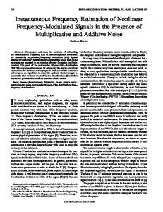
One of the most important application areas of this technology is the imaging and measurement of speech sound. It has been found to be particularly useful for analyzing the fine scale time-frequency features of individual pulsations of the vocal cords during phonation, so one example of this kind of short signal will be adopted as a test signal for the demonstration of the algorithms. The source-filter theory of speech production models phonation as a deterministic process, the excitation of a linear filter by a pulse train. The filter resonances of the mouth “ring” after excitation by each pulse, yielding the formants of a speech sound. One can observe these formants as they are excited by the individual glottal pulsations in Fig. 1, which pictures a portion of a vowel 关e兴 produced with creaky phonation having extremely low airflow and fundamental frequency to enhance the accuracy of the source-filter model. 362

J. Acoust. Soc. Am., Vol. 119, No. 1, January 2006

Figure 2 shows a conventional spectrogram of the test signal, which is one vocal cord pulsation excised from the previous signal. This and all subsequent examinations of this signal are computed using 7.8 ms windows and 78 ␮s frame advance. While it is possible to observe the numerous formant frequencies as they resonate, the conventional spectrogram shows an extreme amount of time-frequency “smearing” owing to the short window length employed and high magnification. A major goal of the time-corrected instantaneous frequency spectrogram is to move away from the pure time-frequency domain which attempts to show an energy distribution, and instead work to track the instantaneous frequency of each significant AM/FM line component constituting the signal frames. A. Methods computing the finite difference approximation 1. Spectrogram reassignment

Both the original proposal of Kodera et al.1 and the later independent developments by Nelson2 compute the channelized instantaneous frequency and local group delay using their definitions in Eqs. 共2兲 and 共3兲 by means of finite difference approximations. The only real disparity between the two approaches is in the details of how to compute this finite difference, so they can be described with a single algorithmic out-line. It can be presumed that Kodera et al.1 computed the finite differences of the short-time Fourier transform phases literally, e.g., CIF共␻,T兲 = ⬇

⳵ arg共STFTh共␻,T兲兲 ⳵T

冋冉

冊 冉

1 ⑀ ⑀ ␾ T + ,␻ − ␾ T − ,␻ ⑀ 2 2

冊册

.

共4兲

With the CIF and LGD matrices in hand, the frequency and time locations of each point in the digital short-time Fourier transform of the signal are reassigned to new locations according to 共␻,T兲 哫 关CIF共␻,T兲,T + LGD共␻,T兲兴.

共5兲

This form of the reassignment is obtained when the shorttime Fourier transform of the signal f共T兲 is defined following Nelson2 as STFTh共␻,T兲 =

冕

⬁

f共t + T兲h共− t兲e−i␻tdt.

共6兲

−⬁

This form of the transform is equivalent modulo a phase factor ei␻t to the more standard form in which the window is time-translated with the signal held to a fixed time. This important difference between the two forms of the short-time Fourier transform propagates into the local group delay in the expressions and algorithms presented here, so that the value computed from the phase derivative of the abovedefined short-time Fourier transform provides a correction to the signal time for the reassignment rather than a new time value that supersedes the signal time. A later approach to reassigning the power spectrum and spectrogram using the same general ideas was developed by Fulop and Fitz: Computing time-corrected frequency spectrogram

The primary insight of Nelson was that each of the two partial derivatives of the short-time Fourier transform phase can be estimated by means of point-by-point multiplication of two related transform surfaces. Nelson2 states that the self-cross-spectral surface C defined in Eq. 共7兲 encodes the channelized instantaneous frequency in its complex argument, and that analogously the surface L defined in Eq. 共8兲 encodes the local group delay in its complex argument,

冉

C共␻,T, ⑀兲 = STFT ␻,T +

FIG. 1. Vocal cord pulsations during a creaky voiced production of the vowel 关e兴, “day,” wave form and conventional spectrogram shown.

Nelson.25,26,2 Nelson’s stated goal was the estimation of the desired partial derivatives without finite differencing, since it was assumed that phase unwrapping was important in extracting acceptable performance from that method, and phase unwrapping can present well-understood difficulties in certain circumstances.

冉

⑀ ⑀ STFT* ␻,T − , 2 2

冊 冉

冊

共7兲

冊 冉

冊

共8兲

⑀ ⑀ L共␻,t, ⑀兲 = STFT ␻ + ,T STFT* ␻ − ,T . 2 2

Let us demonstrate that the argument of C does indeed provide the same approximation to the STFT phase derivative as the finite difference, since no derivation can be found in the literature:

FIG. 2. Conventional spectrogram of a single vocal cord pulsation from the vowel 关e兴. Computed using 7.8 ms windows and 78 ␮s frame advance. J. Acoust. Soc. Am., Vol. 119, No. 1, January 2006

Fulop and Fitz: Computing time-corrected frequency spectrogram

363

冉 冉 冊 冉 冊冊 冉冉 冊 冉 冊

1 1 ⑀ ⑀ arg关C共␻,T, ⑀兲兴 = arg STFT ␻,T + STFT* ␻,T − ⑀ ⑀ 2 2 =

共9兲

1 ⑀ ⑀ arg M ␻,T + e j␾共␻,T+⑀/2兲M ␻,T − e−j␾共␻,T−⑀/2兲 ⑀ 2 2

冊

共10兲

where M共·兲 is the magnitude of the short-time Fourier transform and ␾共·兲 is its phase, =

冉冉

and because M is always real, =

冊冉

冊

冊

1 ⑀ ⑀ arg M ␻,T + M ␻,T − e j关␾共␻,T+⑀/2兲−␾共␻,T−⑀/2兲兴 , ⑀ 2 2

冋冉

冊 冉

1 ⑀ ⑀ ␾ ␻,T + − ␾ ␻,T − ⑀ 2 2

冊册

共12兲

.

An analogous derivation holds for the other surface L. Given this, it is possible to write the following estimates: CIF共␻,T兲 ⬇

1 arg关C共␻,T, ⑀兲兴, ⑀

LGD共␻,T兲 ⬇

−1 arg关L共␻,T, ⑀兲兴. ⑀

共11兲

共13兲

共14兲

It is important to note that in a digital implementation of Nelson’s procedure the resulting CIF and LGD values are approximations to the same degree of precision as with the original method of Kodera et al.,1 but this procedure automatically takes care of phase unwrapping. It might also be noted that while the reassigned locations of STFT magnitudes computed here do diminish unwanted time-frequency smearing and focus tightly on individual components, two components cannot be separated if they are closer than the classical uncertainty limit that is determined by the length of the analysis window, as was first elucidated by Gabor.6

form matrices; each column is fftn-length Fourier transform of a signal frame computed with a fast Fourier transform function called fft. The length value fftn is supplied by the user. The difference between fftn and winគsize is zero-padded up to fftn for the computation. STFTdel= fft共Sdel兲 STFT= fft共S兲 STFTfreqdel is just STFT rotated by one frequency bin—this can be accomplished by shifting the rows in STFT up by one step and moving the former last row to the new first row. 共3兲 Here are the computational steps at which the original proposal and Nelson’s method differ. 共a兲 In the original method, compute the channelized instantaneous frequency matrix by a direct finite difference approximation. It is possible to define the phase angle in relation to the usual principal argument 共required to be a value between −␲ and ␲ here兲 so that phase unwrapping is a byproduct 共taking the principle angle mod 2␲ should do the trick, so long as the mod function output is defined to take the sign of its second argument兲,

2. Algorithm using the finite difference approximations

The input to the procedure is a signal; its output is a time-corrected instantaneous frequency spectrogram, presented as a three-dimensional 共3D兲 scatterplot showing time on the x axis, channelized instantaneous frequency on the y axis, and short-time Fourier transform log magnitude on the z axis. The plotted points can have their z-axis values linked to a colormap, and then when the 3D plot is viewed directly down the z axis the image will look similar to a conventional spectrogram. 共1兲 First, one builds two matrices S and Sdel of windowed signal frames of length winគsize 共user-supplied to the procedure兲 time samples, with Sdel having frames that are delayed by one sample with respect to S. For the present purposes a standard Hanning window function will suffice, but other windows may be more appropriate for other applications. The windowed signal frames overlap by the same user-input number of points in each of the matrices. 共2兲 One next computes three short-time Fourier trans364

J. Acoust. Soc. Am., Vol. 119, No. 1, January 2006

CIF =

− Fs ⫻ mod共共arg共STFTdel兲 − arg共STFT兲兲,2␲兲, 2␲ 共15兲

where Fs is the sampling rate 共in Hz兲 of the signal. This yields a matrix of CIF rows, one for each frequency bin 共discrete channel兲 in the STFT matrices. 共b兲 Alternatively, compute Nelson’s cross-spectral matrix: C = STFT⫻ STFTdel*, where the notation X* for complex X indicates the complex conjugate 共pointwise if X is a matrix of complex numbers兲. The notation A ⫻ B for matrices A , B denotes a pointby-point product, not a matrix multiplication. C is a matrix of complex numbers; each row’s phase angles equal the channelized instantaneous frequencies in the channel indexed by that row. Then compute the channelized instantaneous frequency: Fulop and Fitz: Computing time-corrected frequency spectrogram

FIG. 3. Time-corrected instantaneous frequency spectrogram computed with finite difference approximations.

CIF =

Fs ⫻ arg共C兲, 2␲

共16兲

where Fs is the sampling rate 共in Hz兲 of the signal. 共4兲 Compute the local group delay matrix by finite difference approximation, analogously. 共a兲 For the original method: LGD =

fftn ⫻ 共mod共arg共STFTfreqdel兲 2␲Fs − arg共STFT兲兲,2␲兲.

共17兲

This yields a matrix of LGD columns, one for each time step in the STFT matrices. 共b兲 Alternatively, compute Nelson’s cross-spectral matrix: L = STFT⫻ STFTfreqdel* L is also a matrix of complex numbers; each column’s phase angles equal the local group delay values over all the frequencies at the time index of the column. Now compute the local group delay: LGD =

− fftn ⫻ arg共L兲. 2␲Fs

共18兲

For subsequent plotting, each STFT matrix value is positioned on the x axis at its corrected time by adding to its signal time the corresponding 共i.e., coindexed兲 value in the LGD matrix, plus an additional time offset equal to winគsize/2Fs. The offset is required because this LGD computation corrects the time relative to the leading edge of the analysis window, but it is conventional to reference the signal time to the center of the window. Each STFT matrix value is positioned on the y axis at its instantaneous freJ. Acoust. Soc. Am., Vol. 119, No. 1, January 2006

quency value found at the coindexed element in the CIF matrix. 3. Performance on a test signal

It is apparent from Fig. 3 that, in comparison to the above-shown conventional spectrogram, the instantaneous frequencies of the line components 共vowel formants, in this instance兲 are successfully highlighted, and the time correction by the local group delay is significant and shows the event time of the glottal impulse to a much higher degree of precision. It is important to emphasize that while this technique has been said to “increase the readability of the spectrogram,”3 since it no longer plots a conventional timefrequency representation it also eliminates some spectrographic information such as the spread of energy around the components 共bandwidth兲. 共This “bandwidth” information in a spectrogram is as much or more a result of the window function as it is of the actual energy distribution in the signal, but it could of course be kept and used somehow in a modified TCIF spectrogram if so desired.兲 What is now plotted is the instantaneous frequency of the 共assumed兲 single dominant line component in the vicinity of each frequency bin in the original short-time Fourier transform, the occurrence time of which is also corrected by the group delay. When there is more than one significant line component within one frequency bin, these cannot be resolved, and a weighted average of these will be plotted. When there is not significant energy within a particular time-frequency cell in the shorttime Fourier transform matrix, a point with a meaningless location will be plotted somewhere, but it is not so easy to remove these troublesome points by clipping because the “significance” of a point is relative to the amplitudes of nearby components. A more sophisticated technique for reFulop and Fitz: Computing time-corrected frequency spectrogram

365

moving points that do not represent actual components has been suggested,2,27 but cannot be considered in this paper. The TCIF spectrogram for the above-mentioned signal computed using the Nelson method is by all measures indistinguishable from that shown in Fig. 3, so it would be redundant to print it. After considerable testing, we conclude that the two methods of approximating the phase derivatives are equally successful in practice. In addition, their computational complexity is similar, in that they each require the computation of two short-time Fourier transforms from the signal. The time-corrected instantaneous frequency spectrogram can reasonably be viewed as an excellent solution to the problem of tracking the instantaneous frequencies of the components in a multicomponent signal.24 In many common applications of spectrography 共e.g., imaging and measuring the formants of speech sounds, as well as tracking the harmonics of periodic sounds兲, the solution to this problem is actually more relevant than what a conventional timefrequency distribution shows. In particular it should be emphasized that, while the frequencies that can be measured in a conventional spectrogram are constrained to the quantized frequency bin center values, the channelized instantaneous frequency of the dominant component near a bin is not quantized, and can be arbitrarily accurate under ideal separability of the components, even at fast chirp rates. B. The method of Auger and Flandrin 1. Theory of the method

The method of Kodera et al. was further developed by Auger and Flandrin,3 but the digital implementation details were somewhat difficult to tease out from their theoryfocused paper. Digital implementations 共MATLAB programs兲 which included the ability to create time-corrected instantaneous frequency spectrograms were ultimately released to the public domain by these authors on the Internet and have since been published,4 though these have not been consulted or used here. At the root of this technique there lies a rigorously derived pair of analytical expressions for the desired partial phase derivatives which invoke two new transforms using modifications of the window function h共t兲, viz. a derivative window dh共t兲 / dt and a time-product window t · h共t兲. Referring to the present choice of definition of the short-time Fourier transform in Eq. 共6兲, the Auger-Flandrin equations must be written as follows; note the importance of using two different time variables T and t: CIF共␻,T兲 = I

再

LGD共␻,T兲 = R

冎

STFTdh/dt共␻,T兲 ⫻ STFT*h共␻,T兲 + ␻, 兩STFTh共␻,T兲兩2

再

冎

STFTt·h共␻,T兲 ⫻ STFT*h共␻,T兲 . 兩STFTh共␻,T兲兩2

共19兲 共20兲

These expressions can be sampled in a discrete implementation, to yield values of the derivatives at the STFT matrix points. Thus the resulting CIF and LGD computations are 366

J. Acoust. Soc. Am., Vol. 119, No. 1, January 2006

not estimates in the sense provided by the other two methods. It is easy to show empirically, however, that there is virtually no apparent difference between the results of this method and those of the finite difference methods.

2. Algorithm computing the Auger-Flandrin reassigned spectrogram

共1兲 A time ramp and frequency ramp are constructed for the modified window functions, and these depend in detail on whether there is an odd or even number of data points in each frame. Accordingly, the following algorithm should be used to obtain the ramps and the special windows: 1: if mod共winគsize, 2兲 then 2: Mw = 共winគsize− 1兲 / 2 3: framp= 关共0 : Mw兲 , 共−Mw : −1兲兴 共using MATLAB colon notation for a sequence of numbers stepping by one over the specified range兲 4: tramp= 共−Mw : Mw兲 5: else 6: Mw = winគsize/ 2 7: framp= 关共0.5: Mw − 0.5兲 , 共−Mw + 0.5: −0.5兲兴 8: tramp= 共−Mw + 0.5: Mw − 0.5兲 9: end if 10: Wt= tramp⫻ window 11: Wdt= −imag共ifft共framp⫻ fft共window兲兲兲; 共ifft is the inverse transform function to fft兲 共2兲 One next builds three matrices of windowed signal frames of length winគsize time samples. The matrix S has its frames windowed by the nominal function window. The matrix Sគtime has its frames windowed by Wt, while the matrix Sគderiv has its frames windowed by Wdt. The windowed signal frames overlap by a user-supplied number of points. 共3兲 One next computes three corresponding short-time Fourier transform matrices in the above-described customary manner: STFT= fft共S兲 STFTគtime= fft共Sគtime兲 STFTគderiv= fft共Sគderiv兲 共4兲 CIF = − Fs ⫻

I共STFT គ deriv ⫻ STFT*兲 + fbin 兩STFT兩2 共21兲

where Fs is the sampling rate 共in Hz兲 of the signal and fbin is a column vector of frequency bin values resulting from the Fourier transform, to be added pointwise. Once again the notation A ⫻ B for matrices A , B denotes a point-by-point product. 共5兲 LGD =

R共STFT គ time ⫻ STFT*兲 Fs ⫻ 兩STFT兩2

共22兲

Fulop and Fitz: Computing time-corrected frequency spectrogram

FIG. 4. Time-corrected instantaneous frequency spectrogram computed with the Auger-Flandrin equations.

3. Performance on the test signal

It is sufficient to note for our purposes that any differences that can be detected in any way between Figs. 3 and 4 are very minute and affect chiefly points that show computational artifacts rather than true signal components. No signal has yet been found to betray significant sizable differences between the Auger-Flandrin method and either of the finite-difference methods. Considering the computational load, the last and most exact method requires one more short-time Fourier transform matrix than the other methods. Theoretically the Auger-Flandrin technique is more exact, yet the advantage is in no way apparent for this or any other test signal that we have tried.

To exaggerate the aerodynamic aspect of glottal excitation, one can pronounce a vowel with an obviously breathy voice, in which the vocal cords never completely close during the glottal cycles and an audible flow of turbulent air is permitted to pass through at all times. It has long been known in practical acoustic phonetics that breathy voiced sounds yield formants whose frequencies are more difficult to measure. From Fig. 6 one can see why—the acoustic output of the process no longer conforms to a simple sourcefilter model, and has apparently been modified by other forces. This is expected from basic considerations of aeroacoustics when excitation by sources within the flow 共turbulence兲 competes in importance with the more ideal excitation by vocal cord pulsation.

IV. APPLICATIONS A. Examining phonation

As mentioned earlier, the phonation process involves the repetitive acoustic excitation of the vocal tract air chambers by pulsation of the vocal cords, which in an idealized model provide spectrally tilted impulses. As the test signal shows, the time-corrected instantaneous frequency spectrogram provides an impressive picture of the formant frequencies and their amplitudes following excitation by a single such impulse. The test signal was produced using creaky phonation, which has a very low airflow and is quite pulsatile, to render the process as purely acoustic as possible. Under more natural phonatory conditions, the process is significantly aeroacoustic, meaning that the higher airflow cannot be neglected and has clearly observable effects on the excitation of resonances. The manifold effects can easily be observed by comparing Fig. 5 with any of the preceding, even though the vowel in the former was still pronounced with an artificial degree of vocal cord stiffness. J. Acoust. Soc. Am., Vol. 119, No. 1, January 2006

B. Tracking the pitch of whale songs

One of the main pieces of information about whale songs and calls that interests bioacousticians is of course, the melody, or pitch track, of the songs. Whale songs, however, have infamous features that spoil conventional pitch tracking methods, including intervals of disrupted periodicity and occasional chirps with considerably fast frequency modulation. Figure 7 shows a long frame 共40 ms兲 time-corrected instantaneous frequency spectrogram of a portion of a Humpback whale song 共thanks to Gary Bold of the University of Auckland for sharing this Humpback recording with us兲. The hydrophone signal is quite noisy, but the fundamental and second harmonic of the periodic portions of the song are easy to see and measure in this representation. The initial chirp is too fast for conventional pitch tracking algorithms to follow, but in the figure it is shown as a line component with no difficulty. Fulop and Fitz: Computing time-corrected frequency spectrogram

367

FIG. 5. Time-corrected instantaneous frequency spectrogram of one glottal pulsation from the vowel 关e兴 pronounced with stiff modal phonation. Computed using the Nelson method with 5.9 ms windows and 78 ␮s frame advance.

C. Sound modeling and resynthesis

Sound modeling goes beyond analysis or transformation of the sample data to construct something not present in the original wave form. In sound modeling, one attempts to extract a complete set of features to compose a sufficient description of all perceptually relevant characteristics of a sound. One further strives to give structure to those features such that the combined features and structure 共the model兲 form a sufficient description of a family of perceptually similar or related sounds.

The models are intended to be sufficient in detail and fidelity to construct a perceptual equivalent of the original sound based solely on the model. Furthermore, deformations of the model should be sufficient to construct sounds differing from the original only in predictable ways. Examples of such deformations are pitch shifting and time dilation. Traditional additive sound models represent sounds as a collection of amplitude- and frequency-modulated sinusoids. These models have the very desirable property of easy and intuitive manipulability. Their parameters are easy to under-

FIG. 6. Time-corrected instantaneous frequency spectrogram of one glottal pulsation from the vowel 关e兴 pronounced with breathy phonation. Computed using the Nelson method with 5.9 ms windows and 78 ␮s frame advance.

368

J. Acoust. Soc. Am., Vol. 119, No. 1, January 2006

Fulop and Fitz: Computing time-corrected frequency spectrogram

FIG. 7. Time-corrected instantaneous frequency spectrogram of a song segment produced by a Humpback whale. Computed using the Nelson method with 40 ms windows and 4.5 ms frame advance.

stand and deformations of the model data yield predictable results. Unfortunately, for many kinds of sounds, it is extremely difficult, using conventional techniques, to obtain a robust sinusoidal model that preserves all relevant characteristics of the original sound without introducing artifacts. The reassigned bandwidth-enhanced additive sound model22 is a high-fidelity representation that allows manipulation and transformation of a great variety of sounds, including noisy and nonharmonic sounds. This sound model combines sinusoidal and noise energy in a homogeneous representation, obtained by means of the time-corrected instan-

taneous frequency spectrogram. The amplitude and frequency envelopes of the line components are obtained by following ridges on a TCIF spectrogram. This model yields greater precision in time and frequency than is possible using conventional additive techniques, and preserves the temporal envelope of transient signals, even in modified reconstruction. Figure 8 shows the conventional spectrogram of an acoustic bass tone. The long analysis window is needed to resolve the harmonic components in the decay of the bass tone, which are spaced at approximately 73.4 Hz. This

FIG. 8. Conventional spectrogram of acoustic bass pluck, computed using a Kaiser window of 1901 samples at 44.1 kHz with a shaping parameter to achieve 66 dB of sidelobe rejection.

J. Acoust. Soc. Am., Vol. 119, No. 1, January 2006

Fulop and Fitz: Computing time-corrected frequency spectrogram

369

FIG. 9. TCIF spectrogram of acoustic bass pluck, computed with the same window parameters as Fig. 8.

acoustic bass sound is difficult to model because it requires very high temporal resolution to represent the abrupt attack without smearing. In fact, in order to capture the transient behavior of the attack, a window much shorter than a single period of the wave form 共approximately 13.6 ms兲 is needed, on the order of 3 ms. Any window that achieves the desired temporal resolution in a conventional approach will fail to resolve the harmonic components. Figure 9 shows a TCIF spectrogram for the same bass tone as above. From this reassigned spectral data, a robust model of the bass tone that captures both the harmonic components in the decay and the transient behavior of the abrupt attack can be constructed. Again it is prudent to emphasize that this single attack transient has been located in time to a high level of precision; this is not to suggest that two closely spaced transients could be resolved if they both fell within a single analysis frame. V. CONCLUSION

The time-corrected instantaneous frequency spectrogram has gone by many names, and has so far remained littleknown and underappreciated in the signal processing and acoustic literature. This is suspected to be due to the widely scattered research papers often containing perfunctory explanations of the proper interpretation of this signal representation, and subsequent natural confusion in the community about its precise nature and relationship to well-understood time-frequency representations. In short, the TCIF spectrogram is not an ordinary time-frequency representation at all, in that it is not a two-dimensional invertible transform, or even a two-dimensional function, and it does not endeavor to show the overall distribution of signal energy in the timefrequency plane. Rather, it is a different way of examining 370

J. Acoust. Soc. Am., Vol. 119, No. 1, January 2006

the time-frequency makeup of a signal by showing only the instantaneous frequencies of its AM/FM line components as revealed by a particular choice of analysis frame length. For many applications such as those exemplified here, focusing solely on the line components is oftentimes more valuable than the time-frequency energy distribution. ACKNOWLEDGMENTS

This work was supported in part by a Research Incentive Grant from the University of Chicago Department of Computer Science while S. A. F. was a Visiting Assistant Professor with the Departments of Linguistics and Computer Science. The authors are grateful to Mike O’Donnell for introducing them to each other. 1

K. Kodera, C. de Villedary, and R. Gendrin, “A new method for the numerical analysis of non-stationary signals,” Phys. Earth Planet. Inter. 12, 142–150 共1976兲. 2 D. J. Nelson, “Cross-spectral methods for processing speech,” J. Acoust. Soc. Am. 110, 2575–2592 共2001兲. 3 F. Auger and P. Flandrin, “Improving the readability of time-frequency and time-scale representations by the reassignment method,” IEEE Trans. Signal Process. 43, 1068–1089 共1995兲. 4 P. Flandrin, F. Auger, and E. Chassande-Mottin, “Time-frequency reassignment: From principles to algorithms,” in Applications in TimeFrequency Signal Processing, edited by A. Papandreou-Suppappola 共CRC Press, Boca Raton, FL, 2003兲, pp. 179–203. 5 R. K. Potter, “Visible patterns of sound,” Science 102, 463–470 共1945兲. 6 D. Gabor, “Theory of communication,” J. Inst. Electr. Eng., Part 3 93, 429–457 共1946兲. 7 R. M. Fano, “Short-time autocorrelation functions and power spectra,” J. Acoust. Soc. Am. 22, 546–550 共1950兲. 8 M. R. Schroeder and B. S. Atal, “Generalized short-time power spectra and autocorrelation functions,” J. Acoust. Soc. Am. 34, 1679–1683 共1962兲. 9 R. M. Lerner, “Representation of signals,” in Lectures on Communication System Theory, edited by E. J. Baghdady 共McGraw-Hill, New York, 1961兲, pp. 203–242. Fulop and Fitz: Computing time-corrected frequency spectrogram

10

C. W. Helstrom, “An expansion of a signal in Gaussian elementary signals,” IEEE Trans. Inf. Theory IT-12, 81–82 共1966兲. 11 L. K. Montgomery and I. S. Reed, “A generalization of the GaborHelstrom transform,” IEEE Trans. Inf. Theory IT-13, 344–345 共1967兲. 12 A. W. Rihaczek, “Signal energy distribution in time and frequency,” IEEE Trans. Inf. Theory IT-14, 369–374 共1968兲. 13 J. R. Carson, “Notes on the theory of modulation,” Proc. IRE 10, 57–64 共1922兲. 14 K. Kodera, R. Gendrin, and C. de Villedary, “Analysis of time-varying signals with small BT values,” IEEE Trans. Acoust., Speech, Signal Process. ASSP-26, 64–76 共1978兲. 15 D. H. Friedman, “Instantaneous-frequency distribution vs. time: An interpretation of the phase structure of speech,” in Proceedings of the IEEEICASSP, 1985, pp. 1121–1124. 16 R. G. Stockwell, L. Mansinha, and R. P. Lowe, “Localization of the complex spectrum: The S transform,” IEEE Trans. Signal Process. 44, 998– 1001 共1996兲. 17 S. A. Fulop, P. Ladefoged, F. Liu, and R. Vossen, “Yeyi clicks: Acoustic description and analysis,” Phonetica 60, 231–260 共2003兲. 18 F. Plante, G. Meyer, and W. A. Ainsworth, “Speech signal analysis with reallocated spectrogram,” in Proceedings of the IEEE Symposium on Time-Frequency and Time-Scale Analysis, 1994, pp. 640–643. 19 F. Plante, G. Meyer, and W. A. Ainsworth, “Improvement of speech spectrogram accuracy by the method of reassignment,” IEEE Trans. Speech

J. Acoust. Soc. Am., Vol. 119, No. 1, January 2006

Audio Process. 6, 282–287 共1998兲. S. W. Hainsworth, M. D. Macleod, and P. J. Wolfe, “Analysis of reassigned spectrograms for musical transcription,” in IEEE Workshop on Applications of Signal Processing to Audio and Acoustics, 2001. 21 M. Niethammer, L. J. Jacobs, J. Qu, and J. Jarzynski, “Time-frequency representation of Lamb waves using the reassigned spectrogram,” J. Acoust. Soc. Am. 107, L19–L24 共2000兲. 22 K. Fitz and L. Haken, “On the use of time-frequency reassignment in additive sound modeling,” J. Audio Eng. Soc. 50, 879–893 共2002兲. 23 T. Nakatani and T. Irino, “Robust and accurate fundamental frequency estimation based on dominant harmonic components,” J. Acoust. Soc. Am. 116, 3690–3700 共2004兲. 24 T. J. Gardner and M. O. Magnasco, “Instantaneous frequency decomposition: An application to spectrally sparse sounds with fast frequency modulations,” J. Acoust. Soc. Am. 117, 2896–2903 共2005兲. 25 D. J. Nelson, “Special purpose correlation functions for improved signal detection and parameter estimation,” in Proceedings of the IEEE Conference on Acoustics, Speech and Signal Processing, 1993, pp. 73–76. 26 D. J. Nelson and W. Wysocki, “Cross-spectral methods with an application to speech processing,” in SPIE Conference on Advanced Signal Processing Algorithms, Architectures, and Implementations IX 关Proc. SPIE 3807, 552–563兴. 27 D. J. Nelson, “Instantaneous higher order phase derivatives,” Digit. Signal Process. 12, 416–428 共2002兲. 20

Fulop and Fitz: Computing time-corrected frequency spectrogram

371