Algorithms for Haptic Rendering of CSG Trees

Algorithms for Haptic Rendering of CSG Trees Chris Raymaekers

Frank Van Reeth

Expertise centre for Digital Media, Limburg University Centre Wetenschapspark 2, B-3590 Diepenbeek Belgium E-mail: {chris.raymaekers, frank.vanreeth}@luc.ac.be Abstract We present an algorithm for haptic rendering of CSG models. This algorithm makes use of the normalised and pruned CSG tree as needed by the graphics algorithm, thus not requiring an extra evaluation of the CSG tree. The algorithm also uses a generic implementation of the intersection, subtraction and union operators which do not make any assumptions on their children in the CSG tree, other than their ability to calculate a surface contact point. This allows us to implement extra primitives without making any modifications to the existing algorithm. In order to implement the subtraction operator, we propose a haptic algorithm to render the inside of an object.

2. CSG Trees A CSG model consists of a series of primitives and boolean operators, which are grouped into a tree. Most CSG implementations use the intersection (∩), subtraction (−) and union (∪) operators. An example of such a tree can be seen in figure 1. Such a tree is often written as (A ∩ B) − C or, assuming left association of operators, A ∩ B − C.

1. Introduction Constructive solid geometry (CSG) has proven to be a good metaphor for constructing complex objects. These complex objects are created by applying boolean operations on simple, mathematical objects. For instance, a box with a hole can easily be defined as a cylinder subtracted from a box. The algorithms for interactive rendering of CSG models have been known for a number of years. However, at present no algorithm for haptic rendering of CSG models is reported on. Since force feedback has proven to be beneficial for 3D modelling [5, 9] and virtual prototyping [1, 2, 7] and since CSG has long been used for modelling solid objects, we believe that these techniques should be combined. This paper elaborates on a generic algorithm for haptic rendering of CSG models; this algorithm can make use of any primitive without any modifications of the existing code for the intersection, subtraction and union operators. First, a brief explanation of haptic rendering and CSG trees will be given. Next the algorithms are explained. Finally, the results of the algorithm will be discussed and a conclusion will be given.

Figure 1. Example CSG tree In this CSG tree, the intersection of a cube and a sphere is taken, which results in a rounded cube. Next a hole is created by subtracting a cylinder from this cube. The result of this tree is depicted in figure 2. The usage of CSG trees has a number of advantages [3]: • • • •

Files from a number of applications can be read. CSG trees are accurate. CSG trees can easily be validated. CSG representations are compact.

3. Haptic Rendering of CSG Trees The algorithms for interactive visual rendering of CSG models have been known for a number of years. These algorithms either use special hardware with 2 depth buffers [8] or the stencil buffer available on standard OpenGL graphics boards [10].

The explanation of our algorithms, in the next sections, make use of the objects depicted in figure 3: a sphere and a cube that intersect each other (a cross section is shown).

Figure 2. Result of the CSG tree of figure 1 Techniques needed for haptic rendering differ radically from the graphical techniques. Graphical algorithms make use of the fact that the objects must be projected on a viewport in such a manner that a perspective is maintained in a viewpoint. All graphical CSG algorithms make use of a variation of a ray-casting scheme. However, no haptic equivalent of such a viewport exists: haptic algorithms make objects touchable from all sides, even invisible sides. Our algorithm for rendering CSG trees calculates a surface contact point (SCP) for CSG models. In order to create a set of primitives that can be easily expanded, the algorithms do not make any assumptions on the geometries of the primitives. A primitive has to provide two methods in order to be used in a CSG tree: 1. The primitive has to check if a point lies inside or outside its surface. 2. The primitive has to calculate the SCP if the point lies inside its surface. The algorithms will then combine the surface contact points of the subtrees. The subtraction operator requires an extra functionality, because it has to be able to haptically render the inside of a surface: 3. The primitive has to calculate the SCP if the point lies outside its surface. This requirement differs from requirement 2 because the techniques for rendering the outside of an object differ from the techniques to render the inside of an object. This problem is further discussed in section 3.3. For most primitives the inside-outside test and the calculation of a SCP if the pointer lies inside its surface are well-known and are thus not explained in this paper. We will however elaborate on the calculation of a SCP if the pointer lies outside an object’s surface and on the calculations for the operation nodes.

Figure 3. Example objects

3.1. Intersection The intersection of two objects is formed by the volume that is shared by these objects. As a result, only the surfaces that are shaded black in figure 4 have to be felt. The rendering algorithm should ignore the greyed surfaces.

Figure 4. Intersection of the example objects The algorithm will only calculate the SCP if the pointer is located in the volume that is defined by the black surfaces in this figure. Otherwise, the pointer is considered outside the intersection and no forces should be applied. The inside-outside test for a intersection node should therefore test if an object is located inside the left tree and inside the right tree. Both subtrees are responsible for calculating if the pointer is located within the object represented by the subtree. When the SCP is inside the intersection and thus passed the inside-outside test, the black surfaces are closer than the grey surfaces, so algorithm 1 is valid. The intersection algorithm calculates which of the two SCPs lies closest to the pointer’s position; this SCP is chosen, unless it is too far away from the previous SCP. This extra check is performed to avoid the pointer to pop through an object if too much pressure is applied by the user. The algorithm however, can only assure that this effect is avoided if the primitives do not allow the pointer to pop through themselves: an individual primitive must never allow the pointer

GetIntersectionSCP () { SCP1 = L e f t T r e e . GetSCP ( ) ; SCP2 = R i g h t T r e e . GetSCP ( ) ; d i f f 1 = SCP1 − P o i n t e r P o s i t i o n ; d i f f 2 = SCP2 − P o i n t e r P o s i t i o n ; d i s t a n c e 1 = SCP1 − P r e v i o u s S C P ; d i s t a n c e 2 = SCP2 − P r e v i o u s S C P ; if diff1 . length < diff2 . length if distance1 . length / distance2 . length < threshold r e t u r n SCP1 ; else r e t u r n SCP2 ; else if distance2 . length / distance1 . length < threshold r e t u r n SCP2 ; else r e t u r n SCP1 ; }

surface to another can never be smooth. We can therefore use the previous SCP to ensure that the pointer will not pop through the resulting object. The procedure for rendering a subtraction is given in algorithm 2. GetDifferenceSCP ( ) { SCP1 = L e f t T r e e . GetSCP ( ) ; SCP2 = R i g h t T r e e . G e t I n t e r n a l S C P ( ) ; d i f f 1 = SCP1 − P r e v i o u s S C P ; d i f f 2 = SCP2 − P r e v i o u s S C P ; if diff1 . length < diff2 . length r e t u r n SCP1 ; else r e t u r n SCP2 ; }

Algorithm 2. Subtraction algorithm Algorithm 1. Intersection algorithm

to pop through. The current pointer position, not the previous SCP, is used as the main check, because this would cause the SCP to jitter on transitions from one subtree to the other that should feel like a smooth transition. This is not a problem in the example of figure 4, because the orientations of the surfaces of the sphere and cube differ; the edges in this figure are “hard edges”. However, situations exist where the transition between two objects should either not be felt or should be felt as a slight change in orientation of the surface. Experiments have shown us that a value of 50 is sufficient for the threshold to avoid pop-throughs and does not cause a jitter effect.

The main difference between algorithms 1 and 2 is the haptic rendering of the right subtree: the inside of this subtree’s surface should be rendered, since it is subtracted from the other object and the pointer does not lie inside the right subtree. The next section will discuss the problems that arise when rendering the inside surface of an object.

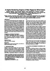
3.3. Internal Rendering of an Object The rendering process for an object’s outside surface is known for a large number of primitives. Figure 6(a) shows how the volume of a cube is divided into 6 segments in the shape of a pyramid. The base of each of these pyramidal segments is a face of the cube; if the pointer enters the segment, the SCP is calculated on this face.

3.2. Subtraction When subtracting an object from another object, the resulting object is defined by the volume of the latter object that is not shared with the former. The inside-outside test of a subtraction node should succeed if the left subtree’s inside-outside test succeeds and the right subtree’s insideoutside test fails. For our example, the resulting object that is formed by subtracting a cube from a sphere is shaded black in figure 5.

(a) Internal segments

(b) External segments

Figure 6. Haptic rendering of a cube (cross section)

Figure 5. Subtracting the example objects Because the object on the right part of the tree is a primitive, as will be explained in section 3.5, the transition of one

The well-known algorithms for rendering objects cannot be used when rendering the inside of the surface if the object’s surface is not continuous. For instance, experiments have shown us the transition between two faces of a cube feels smooth if the segments are expanded into the space outside the cube. Therefore, when the pointer lies outside a cube, a different algorithm must be used to calculate the SCP. Contrary, the rendering algorithm for a sphere is suitable for both rendering the outside and inside surface.

The algorithm for haptic rendering of the internal surface of a cube divides the 3D world into 27 segments (figure 6(b) depicts a cross section of this approach in which 9 segments are shown): • The volume within the cube. This segment is not used for the haptic rendering process since the pointer has to be located outside the cube. Figure 6(b) shows this segment in white. • 6 surface segments. These segments consist of the points that can be projected onto a face of the cube by changing only 1 co-ordinate (x, y or z). Each face has one associated segment. Four of these segments are coloured dark-grey in figure 6(b). • 12 edge segments. The points that can be projected onto the edges by changing two co-ordinates make up these segments. Figure 6(b) displays four edge segments, coloured light-grey.

GetInternalCubeSCP ( ) { f o r each s u r f a c e segment i f P o i n t e r i n segment r e t u r n p r o j e c t i o n of P o i n t e r onto s u r f a c e f o r each edge segment i f P o i n t e r i n segment r e t u r n p r o j e c t i o n of P o i n t e r onto edge f o r each v e r t e x segment i f P o i n t e r i n segment return vertex }

Algorithm 3. Haptic rendering of a cube

3.4. Union The union of two objects is defined as the points in space that are enclosed by either of the objects. The inside-outside test should thus succeed if the inside-outside test of one of the subtrees succeeds. The surface that should be felt for the example objects is coloured black in figure 7.

• 8 vertex segments. Points, whose x, y and z coordinates fall outside the range defined by the cube are projected onto the nearest vertex. These segments are not shown in figure 6(b). Experiments show that, contrary to the extension of the internal algorithm, the above-mentioned procedure ensures that the edges of the cube are felt as hard edges. In general, the inside surface of an arbitrary primitive, consisting of a number of continuous surfaces, can be rendered by dividing space into several segments: one segment for the internal volume of the primitive, one segment for each continuous surface and one segment for each transition between surfaces (both edges and vertices). The rendering algorithm for a sphere that was mentioned earlier is thus a special case of the general approach: only two segments are defined, the internal segment and the external segment for the surface of the sphere. Using the same algorithm, one can see that the haptic rendering process for a cylinder divides space into 6 segments: • The volume within the cylinder. • The volume around the side of the cylinder. • The two volumes that are the extensions of the top and bottom of the cylinder. • The two remaining volumes that are associated with the circles that define the edges between the side and the top and bottom of the cylinder. Algorithm 3 shows a general algorithm for the haptic rendering of the inside surface of an arbitrary primitive.

Figure 7. Union of the example objects The grey surfaces in this figure define the intersection of the two objects. As already mentioned in section 3.1, if the pointer enters this volume, the SCP of one or both subtrees will be positioned on this intersection surface. Algorithm 4 takes this effect into account in order to avoid the SCP to be positioned inside the object. GetUnionSCP ( ) { SCP1 = L e f t T r e e . GetSCP ( ) ; SCP2 = R i g h t T r e e . GetSCP ( ) ; i f P o i n t e r P o s i t i o n i n L e f t T r e e and P o i n t e r P o s i t i o n not in RightTree i f SCP1 n o t i n R i g h t T r e e r e t u r n SCP1 ; i f P o i n t e r P o s i t i o n n o t i n L e f t T r e e and P o i n t e r P o s i t i o n in RightTree i f SCP2 n o t i n L e f t T r e e r e t u r n SCP2 d i f f 1 = SCP1 − P r e v i o u s S C P ; d i f f 2 = SCP2 − P r e v i o u s S C P ; if diff1 . length < diff2 . length { i f SCP1 n o t i n R i g h t T r e e r e t u r n SCP1 ; } e l s e i f SCP2 n o t i n L e f t T r e e r e t u r n SCP2 ;

Candidate = PreviousSCP + P o i n t e r P o s i t i o n − PreviousPointerPosition ; SCP1 = L e f t T r e e . GetSCP ( ) ; SCP2 = R i g h t T r e e . GetSCP ( ) ; i f ( Candidate in union o b j e c t ) { i f C a n d i d a t e i n L e f t T r e e and Candidate not in RightTree { SCP = L e f t T r e e . GetSCP ( C a n d i d a t e ) ; i f SCP n o t i n R i g h t T r e e r e t u r n SCP ; } i f C a n d i d a t e n o t i n L e f t T r e e and Candidate in RightTree { SCP = R i g h t T r e e . GetSCP ( C a n d i d a t e ) ; i f SCP n o t i n L e f t T r e e r e t u r n SCP ; } d i f f 1 = SCP1 − P r e v i o u s S C P ; d i f f 2 = SCP2 − P r e v i o u s S C P ; if diff1 . length < diff2 . length { i f SCP1 n o t i n R i g h t T r e e r e t u r n SCP1 ; } e l s e i f SCP2 n o t i n L e f t T r e e r e t u r n SCP2 ;

3.5. Tree Normalisation Most graphic rendering algorithms assume that the CSG tree is in normal form. A tree is in normal form when all intersection and subtraction operators have a left subtree that contains no union operator and a right subtree that is simply a primitive [4]. A CSG tree can be converted to a normal form by repeatedly applying the following set of production rules to the tree. These production rules make use of the associative and distributive properties of boolean operations: 1. 2. 3. 4. 5. 6. 7. 8. 9.

X − (Y ∪ Z) → (X − Y ) − Z X ∩ (Y ∪ Z) → (X ∩ Y ) ∪ (X ∩ Z) X − (Y ∩ Z) → (X − Y ) ∪ (X − Z) X ∩ (Y ∩ Z) → (X ∩ Y ) ∩ Z X − (Y − Z) → (X − Y ) ∪ (X ∩ Z) X ∩ (Y − Z) → (X ∩ Y ) − Z (X − Y ) ∩ Z → (X ∩ Z) − Y (X ∪ Y ) − Z → (X − Z) ∪ (Y − Z) (X ∪ Y ) ∩ Z → (X ∩ Z) ∪ (Y ∩ Z)

} r e t u r n PreviousSCP ; }

Algorithm 4. Union algorithm If the pointer is located in only one of the two subtrees, the algorithm uses its SCP unless this SCP is located in the other object. Otherwise the closest SCP is used if it is not located in the other object. The other SCP is not considered because this SCP is possibly located on the other side of the union object, thus allowing the pointer to pop through. When the SCPs of both subtrees cannot be used, a heuristic should be used to calculate the exact resulting SCP. This can be done by using numerical methods which make use of knowledge of the primitives, but this is not acceptable because this information is not provided by operation nodes in the subtrees and is not required from the primitives and because these calculations would require a lot of processing time, which would cause the haptic loop to break the 0.9ms restriction. Another, faster method is thus needed. The algorithm calculates a “candidate” SCP by moving the previous SCP in the same direction as the pointer. This candidate is then treated as a new pointer position and the same calculations are made on this candidate. If this step also fails, the algorithm stops in order to respect the timing constraints and using the previous SCP. The proposed algorithm does not always return the exact SCP, but can give a good approximation. Experiments have shown that the errors are smaller than the resolution of the PHANToM device, which is 0.03mm and are thus hardly noticeable.

Normalisation may add a number of nodes to the tree. Some of these nodes do not contribute to the final (graphical and haptic) rendering process. By calculating the bounding volume of the nodes, some nodes may be pruned. The following rules are applied for the operator nodes: 1. Bound(A ∪ B) = Bound(Bound(A) ∪ (Bound(B)) 2. Bound(A ∩ B) = Bound(Bound(A) ∩ (Bound(B)) 3. Bound(A − B) = Bound(A) An intersection node can be pruned if the bounding boxes do not intersect. Likewise, the right subtree of a subtraction node can be pruned if the bounding boxes do not intersect. The third requirement from section 3 implies that a subtraction node’s right subtree is a primitive since the algorithms for the operation nodes do not guarantee that the inside of the surface is rendered properly. This is the only requirement that the haptic rendering process demands. The normalised tree can thus also be used for haptic rendering. However, the union algorithm requires its subtree to calculate the inside-outside test and the SCP a number of times. The normalisation process brings the union operators to the root of the CSG tree, which causes the underlying tree to be calculated several times. Although it is not necessary, processor time can be saved by using an alternative normalised tree for haptic rendering. This tree is calculated by using only a subset of the production rules: 1. X − (Y ∪ Z) → (X − Y ) − Z 2. X − (Y ∩ Z) → (X − Y ) ∪ (X − Z) 3. X − (Y − Z) → (X − Y ) ∪ (X ∩ Z)

The application of this subset leads to a tree that is smaller than the normalised tree; in worst case it is just as large as the normalised tree. Just like the normalised tree, this “subnormalised” tree can be pruned using the rules mentioned earlier.

4. Results We implemented the CSG algorithms using the eTouch [6] library. A PHANToM Premium 1.5A was used as haptic device. This device was attached to a Pentium III, 863 MHz computer with 128 MB RAM, running Windows NT. The graphical output was rendered using OpenGL and the algorithm described in [10]. The different algorithms were assessed by looking at the haptic load when making the calculations. The haptic load is defined as the percentage of the processor time that is needed to perform the haptic algorithms. This haptic load includes (but is not limited to) the time needed to read the haptic device’s encoders, to evaluate the haptic scene graph and to sent force back to the device. Since the haptic loop must be performed at a rate of 1kHz, the haptic load is a considerable percentage. Because the haptic loop is executed 1000 times per second and because the other threads and programs must have time to execute, the haptic loop should not take more than 90ms. Unfortunately, at this moment, no exact measurement of the haptic load is available since the haptic loop is shielded from the user (one can only write extensions of the haptic loop). The PHANToM device drivers, however, include a utility that visually shows the haptic load. Since this is the only way to assess the haptic load, this tool is currently considered a valid (although not precise) means to measure the performance of haptic algorithms. All values that are mentioned in this paragraph are estimates from this visual output; no exact figures can be given. CSG expression Empty scene Sphere Internal sphere Cube Internal cube Cylinder Internal cylinder Object from figure 1

No touch ±25% < 30% < 30% < 30% < 30% < 30% < 30% ±30%

Touch N/A ±30% ±30% ±30% ±30% ±30% ±30% ±35%

Table 1. Comparison of haptic load Table 1 compares the haptic load for some primitives (both “normal” rendering and rendering of the inside of the primitive’s surface) and the CSG tree from figure 1. As an extra comparison, the haptic load for an empty scene graph is also given. The second column of this table gives the

haptic load when the object is not touched. This means that only the inside-outside test is performed. The third column summarises the haptic load when the pointing device touches the object, thus also requiring the calculation of a SCP. Since an empty scene requires a haptic load of ±25% and the haptic load must always be less than 90%, ±65% of the processor time is still available for the calculation of the CSG tree’s SCP. Table 1 shows that our algorithms stay well under the haptic load of 90%.

5. Conclusions We have implemented algorithms that are needed for haptic rendering of a CSG tree. These algorithms make use of the same representation as the graphical rendering algorithms. These algorithms do not make any assumptions on the primitives, other than that a primitive renders its surface contact point in a correct manner. However, the subtraction algorithm also requires that a primitive is able to haptic render the inside of its surface. Finally, we have experimentally shown that the CSG algorithms do not drastically increase the haptic load of an application.

References [1] T. Antilla. A haptic rendering system for virtual handheld electronic products. VTT Publications 347, Technical Research Centre of Finland, 1998. [2] E. Chen. Six degree-of-freedom haptic system as a desktop virtual prototyping interface. In Proceedings of the First International Workshop on Virtual Reality and Prototyping, pages 97–106, Laval, FR, June 1999. [3] J. D. Foley, A. van Dam, S. K. Feiner, and J. F. Hughes. Computer graphics: principles and practice. Systems Programming Series. Addison-Wesley, 1990. [4] J. Goldfeather, S. Molnar, G. Turk, and H. Fuchs. Near realtime CSG rendering using tree normalization and geometric pruning. IEEE Computer Graphics and Applications, 9(3):20–27, May 1989. [5] T. Massie. A tangible goal for 3d modeling. IEEE Computer Graphics and Applications, 18(3):62–65, May–June 1998. [6] e-Touch Programmers Guide, 2000–2001. [7] J. K. Salisbury. Making graphics physically tangible. Communications of the ACM, 42(8):74–81, August 1999. [8] N. Steward, G. Leach, and S. John. An improved Zbuffer CSG rendering algorithm. In 1998 Eurographics/SIGGRAPH Workshop on Graphics Hardware, pages 25–30, Lisbon, PT, August 31–September 1 1998. [9] R. J. Stone. Haptic feedback: A potted history, from telepresence to virtual reality. In Proceedings of the Workshop on Haptic Human-Computer Interaction, pages 1–8, Glasgow, UK, August 31–September 1 2000. [10] T. Wiegand. Interactive rendering of CSG models. Computer Graphics Forum, 15(4):249–261, 1996.