has yet designed a complete computer using only adiabatic logic. We have ... by the MIT Reversible Computing project, and will serve as a benchmark test chip ...
AN ADIABATIC LOGIC IMPLEMENTATION OF A REVERSIBLE CELLULAR AUTOMATON Michael P. Frank Nicole Love Arti cial Intelligence Laboratory Massachusetts Institute of Technology Cambridge, MA 02139
ABSTRACT
Adiabatic circuit techniques have lately been a topic of interest in the low-power design community, but nobody has yet designed a complete computer using only adiabatic logic. We have (almost) completed the circuit design and layout of a simple fully-adiabatic processing element (PE) that nevertheless comprises a general-purpose parallel processor when tiled in large arrays. This PE implements the local update rule for Margolus's Billiard Ball Model Cellular Automaton [3], a reversible universal model of computation. The PE is implemented using Younis and Knight's SCRL logic family [1]. Our cell contains just 292 transistors and tiles on a 131 � 117 �m2 grid in the HP14 process. Hand-calculations indicate that our adiabatic circuit can operate with up to about 1000 times the energy e�ciency of the equivalent standard CMOS circuit.
1. INTRODUCTION
Microscopic physical dynamics is invertible, which suggests that an optimal computation technology using this dynamics would be reversible as well [3]. Any operation that is not reversible is required by thermodynamics to dissipate energy kB T ln 2, where kB is Boltzmann's constant and T is the temperature in K, per bit of information discarded. Current computers dissipate far more energy than this, namely 21 CV 2 , where C is node capacitance and V is voltage swing, whenever they change the voltage of an internal node. However, recent developments in the eld of adiabatic circuits have shown that this CV 2 energy per operation is not really necessary. If circuit nodes are charged and discharged gradually and reversibly, they can operate adiabatically (a term from thermodynamics meaning \without heat ow"). Despite the interest in adibatic computation, nobody has yet carried through the exercise of designing a complete computer based on totally reversible adiabatic technology. Such a design would demonstrate the physical realizability of universal reversible computation and give us practice analyzing and programming such computers, which could be useful if we ever do approach the scale where reversibility is required for e�ciency, by the laws of physics. So for our project we decided to design a very simple adiabatic computer, using a fully-adiabatic circuit technology called SCRL (Split-level Charge Recovery Logic) developed earlier at our lab. Later, the design will be fabricated and tested by the MIT Reversible Computing project, and will serve as a benchmark test chip for evaluating SCRL with di�erent adibatic rail driver technologies. To make the project feasible, we chose the simplest par-
allel universal computer model we knew about, namely that of Margolus's Billiard Ball Model Cellular Automaton (BBMCA) [3]. It is not exactly the most convenient computer to program, but it is simple, universal, reversible, and scalable. In the following sections, we note a few facts about SCRL and BBMCA, describe our circuit design and layout, and provide hand-analysis indicating the power savings achieved by our circuit.
2. SCRL
SCRL [1, 2] has several advantages over its predecessors in adiabatic logic. The main one is that SCRL can be pipelined, allowing for continuously-running, sequential adiabatic circuits. This pipelining requires that each gate be paired with another gate to compute the reverse function. Normal SCRL stages cannot compute non-inverting logic functions, but it is actually possible to compute noninverting functions by providing an extra pair of \fast" rails that split before the main rails do, and re-combine after the main ones. (See [1, 2].) These rails can be used to drive an extra level of logic (such as inverters) to feed the inputs of the main logicq. In this way, a single SCRL stage can compute any logic function. We used this trick to help make our circuits simpler. SCRL, along with many other adiabatic circuit families, requires a power supply that can generate many resonant, swinging supply rails with low dissipation. If the power supplies do not have enough e�ciency, that will limit our power savings. The development of a satisfactory power supply is an active research topic, but in this paper we assume it's given.
3. THE BBMCA
In the billiard-ball model of computation, signals are represented by the presence or absence of billiard balls moving along predetermined paths in a grid. A logic gate is a point where two potential ball trajectories interact. Fixed walls bounce signals around. Any reversible sequential logic circuit can be implemented in this model. The BBM cellular automaton simulates the billiard ball model by representing balls and walls as 1s, and empty space as 0s in a grid. The grid is subdivided into 2x2 blocks, in two di�erent alignments of subdivisions, which alternate between cycles, and are o�set from each other by 1 cell in each of the x and y directions. On each cycle, the contents of each block in the array are modi ed according a simple reversible transformation. Figure 1 shows the BBMCA update rules. The rules are applied independently of block orientation. All con gurations
Free motion.
Collision. Figure 1. BBMCA block update rules.
other than those listed remain constant. Fixed features can be constructed out of several adjacent bits that are all on. Bits that are isolated move diagonally through the array. We implement the CA by placing an SCRL processor at the center of every 2x2 block on each of the two alignments. The processor takes its inputs from block's four cells (which are really just wires coming from the processors in the centers of the four overlapping blocks) and produces its outputs in those same cells, but shifted to an alternate bit-plane (another set of four wires going back out to the neighboring processors). The wires going o� the edges of the array can be folded back into the array to connect the two bit-planes, or fed out to neighboring chips in a larger array.
Figure 2. Block diagram of PE cell.
4. CIRCUIT DESIGN
We decided to focus on so-called \3-phase SCRL" [2] for implementing our array because it is the simplest version of SCRL that doesn't depend on dynamic charge storage, and we wanted to be able to run the clocks arbitrarily slowly or stop them altogether without worrying about losing our logic values, in order to make testing easier. One constraint of 3-phase SCRL is that all circular pipelines must be a multiple of 3 stages long. We chose 6 stages for the complete cycle of interaction from a cell to its neighbors and back, with 3 stages in each cell, and all cells identical. The 2-cell loop could perhaps have been accomplished in 3 stages, but it seemed that this would require more fast rails, and two asymmetrically di�erent types of cells.
4.1. Logic Minimization
We spent a fair amount of time early in the project guring out how to implement the BBMCA update rule in 3 SCRL stages using a minimum amount of logic. Initial concepts had 600 transistors, but nally we arrived at a 240-transistor design. However, this did not allow array initialization, so later we tacked extra logic onto the design which increased the count to 292. It's possible to get by with less, but we haven't had time to re-minimize the logic since adding initialization. The initial 240-transistor logic involved stages generating the following signals. The inputs to stage 1 are A; B; C; D.
� Stage 1. A, B, C , D, S = (A + C )(B + D). � Stage 2. A, B , C , D, S , S , Aout = SA + SA(C + BD),
and similarly for Bout , Cout , Dout . � Stage 3. Aout , Bout , Cout , Dout . In this logic, stage 1 is mainly a bu�er, but also generates the S signal which is used in stage 2. Stage 2 does all the real work of computing the update function, and stage 3 is another bu�er. The reason stage 2 must produce S at its output is so that S will be available for use by the reverse half of stage 2, to compute the inverse update function. The new logic is shown in the schematics section.
Figure 3. Stage 1 logic, S = sh + (A + C )(B + D). Gate for computing Aout in stage 2. 4.2. Block Diagram
Figure 2 shows a schematic block diagram of a single processing element cell. Note the three forward stages along the top, and the three reverse stages along the bottom. There is a mistake in this diagram that was added when incorporating initialization circuitry but we have not yet had time to correct it. (The diagram shows the reverse part of the rst stage being identical to the forward stage 3, and vice-versa, whereas this should not actually the case, due to asymmetry in our initialization scheme.) The sh and sh signals down the middle determine whether the array is in initialization mode or computation mode. Along the bottom are shown the 22 SCRL rails that go to each cell: six swinging supply rails and their complements, two \fast" supply rails and their complements for use in stage 2, and three pass transistor control rails and their complements. Not shown are the constant Vdd and GND rails, which go everywhere to set bulk voltage levels, but carry no current (except for that due to diode leakage).
4.3. Schematics
Below are the schematics for the logic in the forward stages. The reverse stages are very similar. We have not yet had time to size the transistors in our design so as to minimize power, but within each gate, we have, for uniformity, sized its transistors so that the worst-case transition times are the same as that of an inverter with a minimum-width NFET and a twice-minimum-width PFET. (The layout does not yet re ect exactly this sizing in all cases.) Figure 3 shows the logic in stage 1 which computes the inverses of the inputs, together with the S (static) signal used in stage 2. Note that S is turned on when in sh (shift) mode. This special case was added to support array initialization. The gure also shows the gate used for computing each second-stage output. Stage 2 includes four repititions of this gate, di�ering as to which inputs are fed to the A; B; C; D
Table 1. Cadence Device Parameters
NMOS PMOS Value Var Value �0 1.1V �0 0.8993 mj 0.726 mj 0.4905 mjsw 0.2451 mjsw 0.2451 Cj 4.67x10?4 F/m2 Cj 8.76x10?4 F/m2 Cjsw 3.20x10?10 F/m Cjsw 2.13x10?10 F/m tox 9nm tox 9nm �n 978.1 cm2 /V2 -s �p 228.5 cm2 /V2 -s Cox 3.89x10?15 F/�m2 Cox 3.89x10?15 F/�m2 k'n 3.80x10?4 A/V2 k'p 8.889x10?5 A/V2 ally the symmetry here is a mistake; we broke the symmetry when we introduced array initialization circuitry late in the design process. This new circuitry should have gone into just the third SCRL stage, but out of habit, we incorporated it symmetrically into the rst and third stages, which doesn't work. Besides this, we are fairly proud of our layout job; transistors are arranged along neat rows of di�usion to minimize junction area and perimiter capacitances, wire routing is neat and orderly, and things are generally packed as tightly as possible to minimize overall cell area. We perhaps spent too much time on layout, but are generally pleased with the results. Var
Figure 4. Gate for computing A0 = sh A + sh C in stage 3.
5. HAND-ANALYSIS
Figure 5. Current cell layout.
pins, plus 5 \fast" inverters for generating the A; B; C; D;S signals from their inverses using the f�2 and f�2t rails, plus one other inverter for generating S on the stage 2 output. Finally, gure 4 shows the gate that is repeated four times (with di�erent pin assignments) in stage 3. This gate selects either A or the bit in the opposite corner of the block for passing through to the output, depending on sh. Thus if sh is on, input bits go to the opposite output bits, enabling the array as a whole to act as one large shift register, which can be used to initialize the array contents.
4.4. Layout
Figure 5 shows our current cell layout, with metal layers 2 and 3 stripped o� for clarity. The inputs are on the left, outputs on the right. The forward stages run left to right across the top, reverse stages right to left across the bottom. The metal2 layer is used for some local connections, but is primarily reserved for horizontal channels across the cell for routing the 26 global signals to all the cells in a row of the array; metal3 is used similarly in vertical stripes to tie rows of cells together. The layout is highly symmetrical due to the fact that the BBMCA update rule is self-reversing so that the reverse SCRL stages are identical to the forward ones. But actu-
Determining the energy/power dissipation for an adiabatic circuit requires a massive amount of hand calculations. Therefore we decided to make several assumptions and approximations to simplify the hand calculations. Producing results which we believe are a rst order approximation of the power/energy dissipation. The initial assumptions consist of ignoring body e�ect and channel length modulation. Our hand calculations begin by determining the capacitive loads on the output of each stage of the circuit. The circuit consists of three forward stages and three reverse stages, there are two possible drivers for each load line, a forward stage gate or a reverse stage gate. The load line drives two stages the following stage and the reverse stage. For example, the capacitance on the load line of Stage 1 consists of the drain capacitance of Stage 1 and Stage 2R and the gate capacitance of Stage 2 and Stage 1R. Using the values shown in Table 1, equation 1, and equation 3 the worstcase capacitance of a load line was determined, CL . The capacitance per signal was calculated to be �170fF.
Cdb = Keq j � Cj � ADn + Keq jsw � Cjsw � PDn (1) � � ?�0 m (�0 ? Vhigh )1?m ? (�0 ? Vlow )1?m Keq = (2) (Vhigh ? Vlow ) (1 ? m) Cg = Cox WL (3) CL is used to determine an estimate of the maximum current being drawn from the rails. In an adiabatic circuit determining the characteristics of the circuit during the transient is extremely di�cult because both the source and the drain are changing. In adiabatic circuits switching the rails slowly produces a smooth transition because the capacitive load has enough time to charge up with the rail. With a slow changing rail the drain follows the source with a small lag, this lag is VDS which will be constant during most of the switching time. We assume the rails are switching slow
Table 2. Adiabatic Edis vs trf
trf Iest VDS Esw /cyc Psw Eleak 1ns 280.5�A 0.22V 2.71pJ 113�W 9.5aJ 10ns 28.0�A 0.021V 264fJ 1.1�W 95aJ 100ns 2.80�A 2mV 26fJ 10.8nW 950aJ 1�s 280nA 207�V 2.6fJ 108pW 9.5fJ 10�s 28.0nA 20�V 260aJ 1.08pW 95fJ 100�s 2.80nA 2�V 26aJ 10.8fW 950fJ 1ms 0.280nA 200nV 2.6aJ 0.108fW 9.5pJ enough to produce a fairly constant VDS which we label as VDSest. We use a crude estimate of the current shown in equation 4 based on the voltage change at the output. With the assumption that the rail is changing slowly this approximation of the current should be close to the average current during the transient. In calculating VDSest we also approximate VGS to be it's value at the halfway mark of the transient, which seems to be a fair approximation for a rst order approximation. Table 2 shows the results of calculating Iest and VDSest with varying rise/fall times. (4) Iest = CL �Vtout r � � 2 ? � Iest = kp0 WL V GS ? VT VDSest ? VDS (5) 2 r (6) VDSest = V GS ? V GS 2 ? 2 Ikest p The equation used for energy dissipation due to switching of the adiabatic circuit was determined by intergrating the power=IV over the rise/fall time of rails. Using equation 7 the energy per signal per cycle was calculated and is shown in Table 2. The energy?11dissipated due to leakage was calculated using Ileak = 10 A as the leakage current through a transistor (Cadence device characteristics). From the table it is clear that the energy due to switching is proportional to the inverse of trf and the energy due to the leakage is proportional to trf . Therefore equation 9 shows Etot with the proportionality constants Ksw and Kleak referring to the switching and leakage energy respectively. Using this equation the optimum trf can be found which minimizes the energy dissipated by the circuit. (Eswdis =signal) =cycle = Etot = Etot = trf opt = tcycleopt =
2Iest VDSesttrf (7) Esw + Eleak (8) Ksw + Kleak trf (9) trf 523ns (10) 24trf = 12:5�s (11)
In comparison, implementing the same circuit using conventional CMOS required 4 stages corresponding to the three stages and the fast stage of the adiabatic circuit. The energy dissipated by the CMOS circuit is given by equation 12. Where the rst term is the energy dissipated due to switching and the second due to short circuit current. Equation 12 assumes worst-case switching activity (i.e. � = 1). In conventional CMOS the reversible stages are not needed therefore the load capacitance of the circuit will be approximately half the capacitance of the adiabatic circuit. The
Table 3. CMOS vs Adiabatic
Var CMOS Adi. Adi./CMOS E (pJ/cyc) 21.4 9.9x10?3 1/2164 prop. del.(ps) 238 6240 26 worst E (pJ/cyc) 21.4 10.38 .5 total energy dissipated per cycle for the convntional CMOS circuit is 21.4pJ/cycle. The propagation delay of the conventional CMOS circuit using equation 13 is 59.5ps/stage therefore the total propagation delay for the four stages is 238ps. The propagation delay for the adiabatic circuit using the same equation is 260ps/edge and there are 24 edges used to propagate through the three stages, therefore the total propagation delay is 6240ps. Table 3 is a summary of the comparison of the conventional CMOS vs. an adiabatic version. The conventional CMOS circuit has a propagation delay which is more than 26 times less than the propagation delay of the adiabatic circuit. The energy savings of � 2000!!! by the adiabatic circuit over the conventional CMOS circuit is enormous. The worst-case energy dissipation for the adiabatic circuit is assuming that the power supplies are switching instantaneously and therefore the same equation used for energy dissipation due to switching can be used as an approximation for the adiabatic circuit. The worst-case energy dissipation is 10.38pJ/cycle.
Etot =cycle = 12 CL Vdd 2 + trf Ipeak Vdd td = CL (VI2 ? V1 ) av
(12) (13)
6. CONCLUSION
We have created the world's rst complete (though still slightly buggy) circuit- and layout-level design for a fully adibatic and reversible universal computer. The architecture is parallel and scalable to arbitrarily large arrays, assuming power supply inputs are repeated periodically. (Global timing skew is not an issue since all data interconnections are local.) We have thus provided the rst concrete example of a piece of hardware that can be programmed to perform arbitrary computations using arbitrarily little energy per operation (ignoring leakage). Even when actual leakage factors are taken into account, our circuit can still operate with less than one thousandth of the energy per operation of a traditional circuit implementing the same computation model. Assuming adequate power supplies can be built, our design and analysis illustrate the enormous power bene ts that can be gained by computing adibatically.
REFERENCES
[1] Younis, S. G. and Knight, Jr., T. F., \Asymptotically Zero Energy Split-Level Charge Recovery Logic." International Workshop on Low Power Design, pp. 177{182, 1994. http://www.ai.mit.edu/people/tk/ lowpower/low94.ps
[2] Younis, S. G., Asymptotically Zero Energy Computing Using Split-Level Charge Recovery Logic, Ph.D. Thesis, MIT Arti cial Intelligence Laboratory, 1994. [3] Margolus, N. H., Physics and Computation, Ph.D. Thesis, MIT Physics Department, 1987.