converge the bound state energies to within a fraction of an meV of the exact energies. As the ..... accuracy because of the large storage sizes required. At best ...
An efficient method for calculating electronic states in self-assembled quantum dots Mervyn Roy and P A Maksym Department of Physics and Astronomy, University of Leicester, University Road, Leicester, LE1 7RH, UK. It is demonstrated that the bound electronic states of a self-assembled quantum dot (SAQD) may be calculated more efficiently with a harmonic oscillator (HO) basis than with the commonly used plane wave basis. First, the bound electron states of a physically realistic self-assembled quantum dot model are calculated within the single-band, position-dependent effective mass approximation including the full details of the strain within the self-assembled dot. A comparison is then made between the number of states needed to diagonalise the Hamiltonian with either a HO or a plane wave basis. With the harmonic oscillator basis, significantly fewer basis functions are needed to converge the bound state energies to within a fraction of an meV of the exact energies. As the time needed to diagonalise the matrix varies as the cube of the matrix size this leads to a dramatic decrease in the computing time required. With this basis the effects of a magnetic field may also be easily included. This is demonstrated, and the field dependence of the bound electron energies is shown.
I.
INTRODUCTION
Self-assembled quantum dots (SAQDs) are fully quantised atom-like systems in the solid state. Over the past decade there has been a large amount of interest in these structures, mainly due to the potential for applications, for example in quantum information processing and optoelectronic devices. Until recently, progress in the field was hampered by the need to study large ensembles of dots and consequently, average dot properties. However, due to advances in experimental techniques it is now possible to study individual dots in detail. Photoluminescence experiments on single self-assembled dots can resolve the many particle energy levels to within a fraction of an meV [1]. Scanning tunnelling spectroscopy [2] and magneto-tunnelling experiments [3] have been used to directly image the single particle bound states within individual SAQDs, whilst, most importantly, STM images of cleaved quantum dots have been used to provide detailed physical information on the shape, size and composition profile of the dots [4]. This additional information has demonstrated that the bound state wavefunctions of SAQDs are significantly affected by the physical dot structure. To calculate the single particle energies to the accuracy now required by experiment, the details of the physical dot structure and most importantly, the strain within each SAQD must be included in the calculation. We propose an efficient method of calculating the electronic states in SAQDs by expanding the SAQD state in terms of harmonic oscillator (HO) functions. The motivation being that the actual localised states of the dot may be represented using fewer basis functions if the basis is already localised on the appropriate length scale. To our knowledge, no other calculations of the bound state wavefunctions of physically realistic SAQD models have been performed with a HO basis. Instead most work has focused on the expansion of the SAQD states in terms of plane waves [5–7], or the solution of the discretised Schr¨odinger equation in real space [8]. Both these methods can be computationally expensive. In this paper we calculate the bound states of a physically realistic model of a SAQD. The calculation is performed within the single-band effective mass approximation including the position dependence of the effective mass and the effect of the strain field within the system. The bound electron wavefunctions are calculated by exact diagonalisation of the Hamiltonian. A comparison is then made between the convergence of the calculation with a harmonic oscillator basis and the convergence with a plane wave basis. We show that the advantages of the harmonic oscillator basis are twofold. First, the bound state energies are found to converge much more rapidly with the HO basis. We demonstrate that the ground state energy may be calculated to within 1% with only a few tens of HO states as compared to a 3 few thousand plane wave states. As the time taken to diagonalise an Nbs × Nbs matrix scales as Nbs this leads to a dramatic reduction in the required computing time. Second, it is relatively straightforward to include the effects of magnetic fields in the calculation with the HO basis. In this paper we calculate the field dependence of the bound electron states between 0 and 20T.
2 II. A.
METHOD The dot model
Throughout this work we use a dot model with dimensions and composition identical to those measured by Bruls et al [4] using cross sectional scanning tunnelling microscopy. The physical description of the dot provided by Bruls et al is very detailed and is therefore used as an example of a typical dot. The calculational methods described in this paper are, however, completely general and may be used to calculate the bound states within SAQDs of arbitrary shape, size and composition profile. The Bruls dot (see Fig. 1) is a square based truncated pyramidal Inc Ga1−c As dot with an Indium fraction varying linearly from c = 0.6 at the base of the dot to c = 1 at the top of the dot. The SAQD rests on a 0.6 nm InAs wetting layer and is surrounded by a GaAs matrix. The dot base is 18 nm x 18 nm, the dot height is 5 nm and the top surface has dimension 10.6 nm x 10.6 nm. The origin of the co-ordinate system used is taken to be at the centre of the Inc Ga1−c As dot with the z direction defined as the growth direction. The x and y axes are aligned with the edges of the dot base. In this model the GaAs cap and substrate have height 30 nm and the entire heterostructure has a square base of 140 × 140 nm. The conduction band offset between GaAs and InAs is taken to be 0.797 eV, with bulk electron effective masses in GaAs and InAs of 0.067 mo and 0.023 mo respectively. To obtain the relevant parameters in the Inc Ga1−c As material we linearly interpolate the effective electron masses, and calculate the conduction band offset in eV with an empirical relation from Barker [6], Vo = −1.178c + 0.381c2.
(1)
The composition and the conduction band offset both vary with position. B.
Solution of the Schr¨ odinger equation
To calculate the bound energy levels and the electron wavefunctions we use the single-band effective mass approximation to the Schr¨odinger equation, HΨ = EΨ, � � 1 −1 (−i¯ h∇ + eA)M (−i¯h∇ + eA) + V (r) Ψ = EΨ, 2
(2)
where M is the effective mass tensor and A is the vector potential related to the magnetic field by B = ∇ × A. V (r) is the electron confinement potential, V (r) = Vo (r) + Vc (r), where Vc (r) is the contribution to the potential due to the strain. The piezoelectric potential is not yet included in this work, however we expect its inclusion to have no effect on the convergence rates investigated. The change in the absolute energies of the bound states caused by the piezoelectric potential is thought to be small [9]. The lattice constant of InAs is 6.7% larger than that of GaAs, consequently the SAQD system is highly strained. The strain field affects the band gaps in the dot and substrate material and hence alters the confinement potential and the effective masses throughout the heterostructure. The relations between the hydrostatic (ǫh ) and biaxial (ǫb ) strains and the strained confinement potentials for electrons, heavy holes (Vhh ) and light holes (Vlh ) are well documented in the literature [10], Vc (r) = ac ǫh (r), b Vhh (r) = av ǫh (r) + ǫb (r), 2 b (3) Vlh (r) = av ǫh (r) − ǫb (r). 2 Then, given the strained potentials, the strained effective electron masses may be evaluated from first order perturbation theory [10], m∗z (r) = m∗ m∗xy (r) = m∗
Vc + EgGaAs − Vlh , Eg (Vc + EgGaAs − Vhh )(Vc + EgGaAs − Vlh ) Eg (Vc + EgGaAs − 34 Vlh − 41 Vhh )
,
(4)
3 where, m∗ , m∗z and m∗xy denote bulk, perpendicular and in-plane effective masses. Vc , and hence the calculated bound state energies are specified with an energy zero at the GaAs conduction band edge. Finally, in units of eV, the band gap, Eg , and the deformation potentials, ac , av and b, in Inc Ga1−c As are [10], Eg ac av b
= = = =
0.41c + 1.52(1 − c), −5.08c − 7.17(1 − c), 1.00c + 1.16(1 − c), −1.80c − 1.70(1 − c).
(5)
Given the position-dependent confinement potentials and effective masses we can always solve Eq. (2) by expanding the exact wavefunction, Ψ, in terms of an arbitrary set of basis functions, ψi , and eigenvectors, ai , X ai ψi , (6) Ψ= i
and then diagonalising the resultant Hamiltonian matrix. C.
Harmonic oscillator basis
In cylindrical polar co-ordinates we may write the actual single particle states of the dot as a sum of harmonic oscillator functions, Ψ(r) =
X
ai ψi =
lX max
mX max nX max
ali mi ni Φli (φ)Zmi (z)Rni li (r)
(7)
li =−lmax mi =0 ni =0
i
where, the ali mi ni are expansion coefficients, and we have used Nbs = (2lmax + 1)(mmax + 1)(nmax + 1) basis functions to approximate the full single particle wavefunction. The individual basis functions in Eq. (7) are given by, 1 Φli (φ) = √ eili φ 2π � � 12 2 2 λz √ Zmi (z) = Hmi [(z − zo )λz ] e−(z−zo ) λz /2 , 2 mi m i ! π � 21 � � � ni !λ2r |li | |li | 1 2 2 − 14 r 2 λ2r (rλ ) L Rni li (r) = e r λ r ni r . 2 2|li | (ni + |li |)!
(8)
|l |
In Eq. (8), Hmi and Lnii are the Hermite and Laguerre polynomials respectively [11] and λz and λr are the reciprocals of the respective length scales of the HO wavefunctions in the parallel and perpendicular directions. The length scales and the offset parameter, zo , can be chosen to optimise the rate of convergence of the HO calculation. Essentially we choose values of λr , λz and zo to give the ground harmonic oscillator basis function a similar spatial extent to the actual localised state of the dot. This is discussed further in section III B. The values of λr are taken to be independent of the magnetic field as the changes in length scales caused by fields of up to 20T are less than 2% and therefore have little effect on the convergence rate. To diagonalise the Hamiltonian (Eq. (2)) and solve for the exact single particle states we must calculate the matrix elements of the Hamiltonian operator between individual HO states (Eq. (7)), Z ∗ (9) Rn∗ j lj (Ho + HB )Φli Zmi Rni li rdrdφdz, Hji = Φ∗lj Zm j where we have split the Hamiltonian into a field independent and a field dependent part, ¯2 h ∇M −1 ∇ + V (r), 2 i¯h 1 i¯ h = − ∇M −1 eA − M −1 A · ∇ + (eA)2 M −1 . 2 2 2
Ho = − HB
(10)
Equation (9) contains terms in which the differential operator acts on products of the inverse effective mass tensor and the basis states. In the present model the effective mass must be calculated numerically, it is therefore advantageous to integrate these terms by parts in order to rearrange the operator order. In this way, the terms containing
4 the differential operator may be written as products of the inverse effective mass tensor and derivatives of the basis functions which may be evaluated analytically. The derivative of the HO function with respect to φ is easily found, whilst the r and z derivatives may be written in a form similar to that of the wavefunctions themselves by using recurrence relations for the Laguerre and Hermite polynomials [11], � 12
dZmi = dz
�
λ3z √ 2 mi m i ! π
dRni li = dr
�
ni !λ4r 2|li | (ni + |li |)!
[2mi Hmi −1 [(z − zo )λz ] − λz (z − zo )Hmi [(z − zo )λz ]] e−(z−zo ) � 12
1
2
2
e− 4 r λr (rλr )|li |−1 � �� 1 |l | −2(ni + |li |)Lnii −1 r2 λ2r . 2
2
λ2z /2
,
�� � � � 1 1 |li | + 2n − r2 λ2r L|lnii | r2 λ2r 2 2 (11)
The field independent matrix elements are then given by, � 2 �� Z � 2 h dψj∗ dψi ¯ ¯h li lj ¯h2 dψj∗ dψi ∗ + V rdrdzdφ. (Ho )ji = + + ψ ψ j i 2m∗xy dr dr 2m∗z dz dz 2m∗xy r2
(12)
With the HO basis it is relatively easy to include the field dependent terms by working in the circular gauge. In cylindrical polar co-ordinates we have, 1 A = (0, Br, 0), 2
(13)
and the matrix elements containing the three field dependent terms are simply, � � Z ¯h(li + lj ) eBr2 eB rdrdφdz. − ψj∗ ψi (HB )ji = 4 2m∗xy m∗xy
(14)
The terms (HB )ij have a very similar form to the matrix elements of the field independent Hamiltonian. The effects of the magnetic field may therefore be included with little additional programming effort and CPU time. D.
Plane wave basis
The Schr¨odinger equation may also be solved by expanding the actual wavefunction in terms of plane waves, Ψ(r) =
X i
ai ψi =
lX max
m max X
nX max
ali mi ni (8Lx Ly Lz )− 2 eiki ·r , 1
(15)
li =−lmax mi =−mmax ni =−nmax
where we have used a total number of Nbs = (2lmax + 1)(2mmax + 1)(2nmax + 1) states in the expansion, and are now working in Cartesian co-ordinates so that r = (x, y, z). The plane wave calculation is carried out with periodic boundary conditions, ki = (ni π/Lx , mi π/Ly , li π/Lz ),
(16)
within a superlattice unit cell of dimension 2Lx × 2Ly × 2Lz . The superlattice unit cell size affects both the converged values obtained for the bound state energies and the rate of convergence of the calculation. This will be discussed in section III C. We must calculate the matrix elements of the Hamiltonian in the plane wave basis. Considering the field independent Hamiltonian and, again integrating by parts so that the differential operators only act on the basis functions, we find, � � Z � 2� kxj kxi + kyj kyi kzj kzi h ¯ −1 + V ei(ki −kj )·r dxdydz. (17) + (Ho )ji = (8Lx Ly Lz ) 2 m∗xy m∗z
5 III.
COMPUTATION
The computational problem was split into three parts. First we calculated the strained confinement potential and effective masses from Eqs. (1), (3) and (4). We then found the relevant matrix elements in the presence or absence of a magnetic field and, finally, diagonalised the Hamiltonian. The diagonalisation was performed with the LAPACK library standard linear algebra routines. We optimised the calculation time for both the HO and the plane wave calculations by considering the symmetry properties of the dot. The Bruls dot belongs to the symmetry group C4v , we, however, use the irreducible representations of the more general symmetry group, C2v , in order to block diagonalise the Hamiltonian into 4 blocks. Each block can then be diagonalised separately, reducing the time taken to fully diagonalise the matrix by up to a factor of 16. Moving from a description of this specific SAQD in terms of the C2v symmetry group to a description in terms of the C4v symmetry group only reduces the time taken to diagonalise the matrix by a factor of about 1.6, at the cost of making the code less general. Both rectangular and square based dots belong to the C2v symmetry group and so the methods used for blocking the matrix may be applied to both types of SAQD. A.
Strain
We calculate the strain within the continuum elasticity approximation with a commercially available, finite element model, Abaqus. This model has already been demonstrated to provide an accurate representation of the strain within a cleaved dot [4]. In this approximation, the system is completely specified in terms of values for the Youngs moduli and Poisson ratios (85.3 Gpa (GaAs), 51.4 GPa (InAs) and 0.32 (GaAs), 0.35 (InAs) respectively [12]) and the lattice mismatch strain (6.7%). As usual we linearly interpolate to obtain the relevant values in the Inc Ga1−c As material. In this paper we are interested in the bound electronic states of an isolated SAQD. We therefore locate the Bruls dot at the centre of a 140 × 140 × 65.6 nm block of semiconductor material and, when calculating the strain, apply periodic boundary conditions to the edges of this block. This system is large enough so that the strain within each dot is unperturbed by the neighbouring dots in the periodic lattice. Figure 2 shows the confinement potential, and the electron effective masses as a function of z through the centre of the dot. The characteristic z dependence of the confinement potential and the effective mass comes mostly from the differences in composition, while the compressive hydrostatic strain inside the dot reduces the electron confinement potential from the unstrained well depth of 0.797 eV. The InAs wetting layer is included as an integral part of this calculation. Its effects on the confinement potential and effective mass can be clearly seen in Fig. 2. B.
Harmonic oscillator basis
To calculate the φ integrals with the HO basis functions we use a fast Fourier transform with 8192 points. The z and r integrals are then calculated using Simpson’s rule on a non-uniform grid, with the highest point densities in the regions where the strained potential varies most rapidly. This gives each matrix element to an accuracy of better than 0.05% The rate of convergence of the harmonic oscillator calculation can be improved by optimising zo and the parallel and perpendicular length scales of the basis states. This is done by minimising the energy of the ground harmonic oscillator state in the dot potential with respect to the HO length scales, and to the offset of the perpendicular R HO states from the centre of the dot, zo . For a given dot we search for the global minimum in Hoo (zo , λr , λz ) = ψo∗ Hψo rdrdzdφ. In the Bruls dot the minimum value of Hoo = −0.218 eV is obtained with zo = −0.25 nm, 1/λr = 3.12 nm and 1/λz = 2.41 nm. Although the convergence rate is improved by optimising these parameters, the rate is not critically dependent on the values chosen for zo , 1/λr and 1/λz , and the final converged values obtained for the bound state energies do not depend on the values chosen for these parameters at all. For example, varying the length scales by 10% changes the value of Hoo by less than 0.1% and therefore gives little difference in the rate of convergence of the calculation. C.
Plane wave basis
The optimum method to calculate the plane wave matrix elements would appear to be a fast Fourier transform. However, using the linear grid required for an FFT it proved impossible to calculate the integrals to the required accuracy because of the large storage sizes required. At best we obtained converged energies only accurate to within a few meV of the actual bound state energies.
6 Instead of the FFT, we therefore used a Simpson’s rule routine to perform each of the integrals. The efficiency of the integration routine was improved by considering the symmetry properties of this particular SAQD: both the x and y integrals are symmetric and real. We estimate that, with this method, we are able to calculate the matrix elements to an accuracy of approximately 0.2%. The plane wave calculation was carried out with periodic boundary conditions within a superlattice unit cell of dimension 2Lz × 2Ly × 2Lx . It was found that the rate of convergence and the converged energies vary according to the box size used. Typically, the smaller the box the faster the convergence, however, with smaller box sizes, the bound wavefunctions within each SAQD are perturbed by the neighbouring dots in the periodic lattice. The converged energies are then smaller than those expected for an isolated SAQD. These effects can be observed in a 1D calculation. Figure 3 shows the calculated ground state energy of electrons confined by the radially averaged confinement potential as a function of the perpendicular box size. The energies calculated with a basis of 200 plane waves vary by less than 0.1% beyond a box size of Lz = 18 nm whilst the convergence using 20 plane waves gets progressively worse at larger box sizes. At small box sizes the calculated ground state energies are much smaller than those of an isolated SAQD. The inset to the plot shows the radially averaged confinement potential in eV referenced to the conduction band offset in GaAs, and the negative of the charge density of the converged ground state calculated using Lz = 30 nm. If the tail of the wavefunction overlaps the edges of the box, the energies converge to lower values than those for an isolated dot. In the 3 dimensional calculation of the electronic states of the Bruls dot we use a box size of Lz = 30 nm, Ly = 30 nm and Lx = 30 nm. However, larger box sizes may be needed to reproduce the isolated dot results for the excited states which have a larger spatial extent than the ground state. IV. A.
RESULTS
Convergence properties
Using the HO basis we calculated the bound state energies of the Bruls SAQD at zero magnetic field. With maximum quantum numbers of lmax = 12, mmax = 20, nmax = 20 and therefore a total number of Nbs = 11025 harmonic oscillator functions in the basis set we found 6 bound states inside the dot. The energies of the bound states are given in table I. The next two most tightly bound states were found to be degenerate and delocalised throughout the wetting layer at an energy of -0.0295 eV relative to the conduction band edge in GaAs. The delocalised states are easily identified by examining the spatial extent of the calculated wavefunctions. Figure 4 shows the rate of convergence of each of the bound states of the Bruls dot. The plot shows the difference in energy between the converged energy and the energies calculated with Nbs basis functions. This is the number of basis functions before the matrix has been blocked. From Fig. 4 we can see the total number of basis states required to obtain any given accuracy. For example, we can obtain ground state energies within 1% of the converged energy with only 24 HO basis states (lmax = 0, mmax = 7, nmax = 2). To calculate the ground state energy to within 1 meV of the converged energy we need 324 basis states (lmax = 4, mmax = 8, nmax = 3). As we would expect, the excited states are slower to converge but we can achieve 1 meV accuracy for all the bound states of the dot with only 1368 basis functions in the expansion. At zero field we also diagonalised the Hamiltonian in a plane wave basis with Nbs = 18081, or maximum quantum numbers of lmax = 20, mmax = 10, nmax = 10 in the z, y and x directions respectively. The energies obtained from the plane wave calculation and the harmonic oscillator calculation typically agree to within a fraction of a percent (see table I). Figure 5 shows the difference in the bound state energies calculated with Nbs plane wave states and those obtained with 18081 plane waves in the expansion. This figure demonstrates that the excited states have clearly not converged, even with a total of 18081 basis functions. The ground state is closer to convergence, but its energy is still decreasing by almost 0.05 meV with the addition of extra in-plane states. To obtain a ground state energy within 1% of the calculated energy found with 18081 basis states we need to include at least 3993 plane waves in the expansion (lmax = 16, mmax = 5, nmax = 5), while to achieve 1 meV accuracy and still retain the C4v symmetry of the dot we need to include a total of 7425 plane waves. The plane wave basis calculation is much slower to converge than the HO calculation. We require at least a factor of 100 more states to obtain convergence to within approximately 1%. The excited state energies found with the plane wave expansion converge to values lower than those obtained from the harmonic oscillator calculation. This indicates that the box size chosen (Lz = Ly = Lx = 30 nm) is too small to completely reproduce the case of an isolated dot. To emphasise that the energies obtained from the plane wave calculation are critically dependent on box size, we recalculated the solutions to the Schr¨odinger equation after setting the inter-dot distance in the periodic lattice to be equal to the dot dimension in each direction. This follows a prescription used by Barker [7] to calculate the bound electron and hole states within a square based pyramidal dot of height 6nm and base 12 nm × 12 nm. With a superlattice unit cell of size Lx = 11.2 nm, Ly = 18 nm, Lz = 18 nm
7 for the plane wave calculation we obtain much more rapid convergence for the states in the Bruls dot. The ground state energy was found to be converged to within 1% of the exact energy with only 91 basis states. However the value obtained for this converged ground state of -0.2472 eV is over 20 meV lower than the ground state energy in an isolated dot. B.
Magnetic field dependence
The bound state energies for the Bruls dot were calculated as a function of magnetic field from 0 to 20 T with 7497 HO states in the expansion to ensure an accuracy to within 0.2 meV for each of the bound states. Figure 6 shows the field dependence of the lowest 8 bound states. Because of the large inter-level spacing, typical of self-assembled dots, the behaviour with magnetic field is relatively simple. We observe crossings between states 7 (dashed line) and 8 (dotted line) at 7.2 T, between states 8 and 6 at 13.1 T and between states 6 and 7 at 18.8 T. We can easily identify crossings and anti-crossings by keeping track of the particular block of the block diagonal Hamiltonian from which each of the bound state energies originates. State 8 (dotted line), one of a pair of degenerate delocalised states at 0 T, becomes bound within the dot above 8.5 T. V.
CONCLUSION
In summary we have demonstrated that the bound electronic states of a self-assembled quantum dot may be calculated more efficiently with a harmonic oscillator (HO) basis than with the commonly used plane wave basis. We calculated the bound electron states within a physically realistic model of a self-assembled quantum dot. The single-band, position-dependent effective mass Hamiltonian was diagonalised with a harmonic oscillator basis and a plane wave basis, and a comparison made between the rates of convergence of the two calculations. It was found that the HO basis gave a much more rapid convergence. Bound state energies within 1 meV of the exact converged energy were obtained with only 324 harmonic oscillator basis functions, while, to achieve similar convergence with a plane wave basis, we required at least 7425 plane waves. This leads to a increase in the computer time needed to diagonalise the Hamiltonian matrix by a factor of approximately 12 ×103 . In both calculations there is also a significant overhead involved in setting up the Hamiltonian matrix which is not affected by the choice of basis. The plane wave basis also has a second disadvantage: The energies obtained are critically dependent on the size of superlattice unit cell used. For example, within a superlattice box chosen to give inter-dot separations equal to the dot dimension we obtained similarly rapid convergence to the HO calculation, but energies which differed from the isolated dot energies by at least 10%. In this paper we have also demonstrated that the effects of a magnetic field may be easily included when working with the HO basis and have shown the field dependence of the bound states between 0 and 20T. Acknowledgements
We would like to thank Dr S P A Gill and Dr F Long of the University of Leicester Engineering department for useful discussions and advice on the strain calculations. This work was performed using the University of Leicester Mathematical Modelling Centre’s supercomputer which was purchased through the EPSRC strategic equipment initiative.
[1] J J Finley, P W Fry, A D Ashmore, A Lemaitre, A I Tartakovskii, R Oulton, D J Mowbray, M S Skolnick, M Hopkinson, P D Buckle and P A Maksym, Phys. Rev. B 63, 161305(R) (2001). [2] U Banin, Y Cao, D Katz and O Millo, Nature 400, 542 (1999). [3] E E Vdovin, A Levin, A Patane, L Eaves, P C Main, Yu N Khanin, Yu V Dubrovski, M Henini and G Hill, Science 290, 122 (2000). [4] D M Bruls, J W A M Vugs, P M Koenraad, M S Skolnick, M Hopkinson, F Long, S P A Gill and J H Wolter, Appl. Phys. Lett. 81, 1708 (2002). [5] M A Cusack, P R Briddon and M Jaros, Phys. Rev. B. 54, R2300 (1996). [6] J A Barker, E P O’Reilly, Physica E 4, 231 (1999). [7] J A Barker, E P O’Reilly, Phys. Rev. B. 61, 13840 (2000). [8] O Stier, M Grundmann and D Bimberg, Phys. Rev. B 59, 5688 (1999).
8 TABLE I: Comparison between the bound state energies calculated with the harmonic oscillator basis (left column) and the plane wave basis (centre column). The energies of the bound states are given relative to the GaAs conduction band edge. State Energy (eV) HO Nbs = 11025 1 -0.2247 2 -0.1563 3 -0.1563 4 -0.0947 5 -0.0720 6 -0.0594
Energy (eV) pw Nbs = 18081 -0.2234 -0.1564 -0.1564 -0.0960 -0.0726 -0.0606
IncGa1-cAs
% difference 0.6 0.1 0.1 1.4 0.8 2.0
GaAs 5
InAs
18
18
0.6
FIG. 1: Schematic of the dot model investigated by Bruls et al.
[9] [10] [11] [12]
M Grundmann, O Stier, and D Bimberg, Phys. Rev. B 52, 11969 (1995). L R C Fonseca, J L Jimenez, J P Leburton and R M Martin, Phys. Rev. B 57, 4017 (1998). M Abramowitz and I A Stegun, Handbook of Mathematical Functions, (Dover Publications, New York, 1965). M R Bruni, A Lapiccirella, G Scavia, M G Simeone, S Viticoli, and N. Tomassini, Thermochemica Acta., 210, 49 (1992).
9
0.08 effective mass (mo)
1.75
V (eV)
1.25 electrons heavy holes light holes
0.75 0.25 −0.25 −20
−10
0 10 z (nm)
20
0.07 0.06
m
* xy
0.05
m
* z
0.04 0.03 −20
−10
0 10 z (nm)
20
FIG. 2: Left: Electron, heavy hole and light hole confinement potentials plotted as a function of z through the centre of the dot. Right: Effective electron masses in units of the bare electron mass.
−0.04
energy (eV)
−0.042 −0.044 0.0 −0.1 −0.2 −0.3 −0.4 −0.5 −0.6 −20
−0.046 −0.048 −0.05 −0.052
0
10
−10
20 30 box size in z (nm)
0
10
40
20
50
FIG. 3: Inset: Variation in radially averaged confinement potential (eV) with z (nm) (solid line). Negative of the charge density of converged ground state in arbitrary units (dashed line). Main figure: Calculated ground state energies for this potential as a function of box size using 200 plane waves (solid line) and 20 plane waves (dashed line).
10
Difference in energy (eV)
0.003
0.002
0.001
0 0
2000
4000
6000
8000
10000
Nbs FIG. 4: Rate of convergence of bound states as a function of number of HO basis functions included in the calculation. Solid line (ground state), dotted line (state 2), points (state 3), dashed line (state 4), long dashed line (state 5), dot dash line (state 6). Horizontal solid lines show energy differences of 0, 0.2 meV and 1 meV between the converged energy and the energies calculated with Nbs basis functions.
Difference in energy (eV)
0.003
0.002
0.001
0 0
5000
10000
15000
Nbs FIG. 5: Rate of convergence of bound states as a function of number of plane wave basis functions included in the calculation. Solid line (ground state), dotted line (state 2), points (state 3), dashed line (state 4), long dashed line (state 5), dot dash line (state 6). Horizontal solid lines show energy differences of 0, 0.2 meV and 1 meV between the energy obtained with 18081 basis states and the energies calculated with Nbs basis functions.
11
0
energy (eV)
−0.05
−0.1
−0.15
−0.2
−0.25
0
5
10 B (T)
15
20
FIG. 6: Field dependence of lowest 8 energy states given by the exact diagonalisation of the single-band Hamiltonian for the Bruls dot. Horizontal solid line shows the cut-off energy for the wetting layer states.