Hindawi Publishing Corporation VLSI Design Volume 2016, Article ID 9532762, 22 pages http://dx.doi.org/10.1155/2016/9532762
Research Article An Efficient Reconfigurable Architecture for Fingerprint Recognition Satish S. Bhairannawar,1 K. B. Raja,2 and K. R. Venugopal3 1
Department of Electronics and Communication, SDMCET, Dharwad 580002, India Department of Electronics and Communication, UVCE, Bangalore 560001, India 3 UVCE, Bangalore University, Bangalore, India 2
Correspondence should be addressed to Satish S. Bhairannawar;
[email protected] Received 7 December 2015; Revised 26 April 2016; Accepted 9 May 2016 Academic Editor: Lazhar Khriji Copyright © 2016 Satish S. Bhairannawar et al. This is an open access article distributed under the Creative Commons Attribution License, which permits unrestricted use, distribution, and reproduction in any medium, provided the original work is properly cited. The fingerprint identification is an efficient biometric technique to authenticate human beings in real-time Big Data Analytics. In this paper, we propose an efficient Finite State Machine (FSM) based reconfigurable architecture for fingerprint recognition. The fingerprint image is resized, and Compound Linear Binary Pattern (CLBP) is applied on fingerprint, followed by histogram to obtain histogram CLBP features. Discrete Wavelet Transform (DWT) Level 2 features are obtained by the same methodology. The novel matching score of CLBP is computed using histogram CLBP features of test image and fingerprint images in the database. Similarly, the DWT matching score is computed using DWT features of test image and fingerprint images in the database. Further, the matching scores of CLBP and DWT are fused with arithmetic equation using improvement factor. The performance parameters such as TSR (Total Success Rate), FAR (False Acceptance Rate), and FRR (False Rejection Rate) are computed using fusion scores with correlation matching technique for FVC2004 DB3 Database. The proposed fusion based VLSI architecture is synthesized on Virtex xc5vlx30T-3 FPGA board using Finite State Machine resulting in optimized parameters.
1. Introduction The reliable personnel authentication [1, 2] based on biometrics has significant importance in the present digital world and can be achieved by human and computer interface activities. The evolution of biometrics in recent years from single mode to multiple mode closed systems has made it possible to consider for Big Data processing [3, 4]. The development of new algorithms and parallel processing architectures has an impact for Big Data processing response time. The interoperable feature and many sources and avenues for collection of biometric samples have made the biometric evolution of Big Data possible. The biometric physiological or behavioural samples are captured using sensors or devices, which are further processed in the next level of vetting through Office for Personal Management (OPM) which can be either verification or identification. Fingerprint based identification is one of the most important biometric
technologies, which have drawn a substantial amount of attention recently since the process of acquiring fingerprint samples are easy and simple. A fingerprint is seen as a set of interleaved ridges and valleys on the surface of the finger. The most fingerprint matching approach relies on the fact that the uniqueness of a fingerprint can be determined by minutiae, which are represented by either bifurcation or termination of ridges. The quality and enhanced minutiae [5–7], which influence recognition rates are discussed in literature. The features of a fingerprint can be derived using the following: (i) Spatial domain: the features of an image are carried out directly on pixel value. Examples are Local Binary Pattern [8], Complete Linear Binary Pattern [9], and Singular Value Decomposition [10]. (ii) Transform domain: in this any transform is applied to an original image to get a transformed image on which further processing is done. Examples are Fast Fourier Transform [11], Discrete Cosine Transform [12], Discrete Wavelet Transform [13], and Dual Tree Complex
2 Wavelet Transform [14]. (iii) Fusion: in this technique [15, 16] it combines the advantages of both spatial and transform domain. The automated fingerprint recognition system is used for both identification and verification against standard database law enforcement agencies to identify the suspect for committing crime or for attendance verification process to verify the claimed identity. The performance speed of fingerprint system is a critical factor to be addressed while dealing with large databases. The real-time processing of a fingerprint recognition system is its ability to process the large data and produce the results within certain time constraints in the order of milliseconds and sometimes microseconds depending on the application and the user requirements. In this category, Field Programmable Gate Array (FPGA) outperforms other processors. The FPGAs are specially built hardware optimized for speed and are suitable for real-time biometric data processing. Multicores and HPC clusters have reasonable real-time processing capabilities, but not efficient as FPGA with many processing cores and high bandwidth memory. In real time, speed of the algorithm becomes crucial which in turn defines the throughput. The efficient FPGA architectures [17–20] for fingerprint processing and existing algorithms to identify a fingerprint based on minutiae [21], ridge, multiresolution features, and Hough transform were discussed. Vatsa et al. [22] proposed Redundant Discrete Wavelet Transform based on local image quality assessment algorithm followed by extraction algorithm using Level 3 features. These features are combined with Level 1 and Level 2 in the fingerprint identification scheme. Finally, the matching performance was improved by using quality based likelihood ratios. Govan and Buggy [23] proposed effective matching solution that addresses security and privacy issues. This technique eliminates the requirement to release biometric template data into an open environment which uses embedded applications such as smart cards. The effective disturbance rejection methodology which is able to differentiate between equivalent and insignificant structure models was discussed. Nain et al. [24] proposed an algorithm to classify fingerprint images into four different classes using High Ridge Curvature (HRC) algorithm involving two stages. In the first stage, HRC region was extracted, which avoids core point detection. In the second stage, ridges inside HRC region were considered for matching. The global distribution structure and the local matching similarities [25] between fingerprints were considered for matching using Hidden Markov Model (HMM) [26]. Nikam and Agarwal [27] proposed spoof fingerprint detection using ridge let transform. The comparisons of individual ridgelet energy and cooccurrence signatures were analysed and also testing was done using diverse classifiers. Masmoudi et al. [28] proposed an algorithm which used the rotation invariant measured as local phase and was combined with Linear Binary Pattern Features to improve the performance accuracy. Stewart et al. [29] proposed the test technique to determine the effects of outdoor and cold weather effects on chip versus optical fingerprint scanner, fingerprint recognition quality, and device interaction. The
VLSI Design results suggested that performance has no dependence on temperature and humidity. Cao and Dai [30] proposed fingerprint segmentation for online process using frame difference technique. Further the segmented foreground was used for identification. Umamaheswari et al. [31] proposed fingerprint classification and recognition using neuro-nearest neighbour based method which improves classification rate. This consists of different stages such as image enhancement, line detector base feature extraction, and neural network classification using back propagation networks. The results have shown the accurate estimation of orientation and ridge frequency which helps in better recognition. Conti et al. [32] proposed pseudo-singularity points based fingerprint recognition. This technique uses additional parameters such as their relative distance and orientation around standard singularity points (core and delta) which enhances the matching performance. Ahmed et al. [33] proposed Compound Local Binary Pattern (CLBP) for rotation invariant texture classification. This combines magnitude information of the difference between two grey values with original LBP pattern and provides robustness. Paulino et al. [34] proposed an alignment algorithm (descriptor-based Hough transform) for latent fingerprint matching. This technique measures similarity between fingerprints by considering both minutiae and orientation field information. The comparison was done between proposed and generalized Hough transform for large database. Feng et al. [35] proposed a technique using orientation field estimation based on prior knowledge of fingerprint structure. The dictionary of reference for orientation patches was constructed using a true set of orientation fields. The approach was applied to the overlapped latent fingerprint database to achieve better performance compared to conventional algorithms. Contribution. The contribution and novel aspects of the proposed techniques are listed as follows: (i) the computation of the novel matching score for CLBP and DWT features; (ii) the matching score values which are varied based on characteristics of images, that is, the values which are computed adaptively based on characteristics of the images; (iii) the fusion of matching scores with improvement factor; (iv) the implementation of FSM based VLSI architecture to improve the hardware performance.
2. Proposed Fingerprint Recognition System An efficient fingerprint recognition model using histogram of CLBP scores, DWT feature scores, and fusion of both scores is given in Figure 1. 2.1. Fingerprint Database. The DB3 of FVC2004 fingerprint database [36] is considered for performance analysis. The size of each fingerprint image is 300 × 480 with 512 dpi. The fingerprint samples of ten different persons are shown in Figure 2.
VLSI Design
3
Training stage CLBP
Histogram
DWT
DWT features
Image resizer (256 × 256) Match score DWT DWT matching
Training samples
Match/ mismatch Recognition stage
Fusion DWT
DWT features
Image resizer (256 × 256)
CLBP matching
CLBP
Match score CLBP
Histogram
Test samples
Figure 1: Block diagram of the proposed fingerprint recognition system.
2.2. Preprocessing. The original fingerprint image of size 300 × 480 is resized to 256 × 256, which is suitable for hardware implementation. 2.3. Complete Local Binary Pattern (CLBP). It is an extension of the Local Binary Pattern (LBP) [37] texture operator. The CLBP operator gives both sign CLBP 𝑆 and magnitude components CLBP 𝑀 for each pixel from its neighbouring pixels. If 𝑃 is the number of neighbours of a centre pixel, then CLBP operator uses 2𝑃 bits to code centre pixel. The first 𝑃 MSB bits represent sign and the next 𝑃 LSB bits represent magnitude. The binary bit patterns are generated for sign and magnitude components for each pixel. The fingerprint image is scanned from left to right and top to bottom and considering each pixel which is surrounded by 8 neighbouring pixels, that is, 3 × 3 matrix. The centre pixel intensity value is 𝐼𝑐 and surrounded neighbouring pixel intensity values, say, 𝐼𝑝 . The sign bit patterns for 3 × 3 matrices are generated using {0, 𝐼𝑝 − 𝐼𝑐 ≤ 0 𝑆 (𝐼) = { 1, 𝐼𝑝 − 𝐼𝑐 > 0. { The magnitude bit pattern is generated using {0, 𝑀 (𝐼) = { 1, {
𝐼𝑝 − 𝐼𝑐 ≤ 𝑀avg 𝐼𝑝 − 𝐼𝑐 > 𝑀avg ,
(1)
(2)
where 𝑀avg = |𝑚1| + |𝑚2| ⋅ ⋅ ⋅ |𝑚8|/8 and 𝑚1 to 𝑚8 are the magnitude values of the difference between respective 𝐼𝑝 and 𝐼𝑐 . Each neighbourhood pixel is represented by two bits; that is, MSB bit represents sign and the LSB bit represents magnitude. Each centre pixel is represented by eight sign bits and eight magnitude bits. The example for CLBP is as shown in Figure 3. The arbitrary values for 3 × 3 matrix are considered in Figure 3(a). The values of neighbouring pixels are subtracted from centre pixel value and are given in Figure 3(b). The sign of each coefficient in Figure 3(b) is represented in Figure 3(c) as sign component of CLBP. The magnitude components of CLBP are shown in Figure 3(d) by considering only magnitude of Figure 3(b). The average value of the CLBP magnitude component is computed and is compared with neighbouring CLBP magnitude coefficient values and assigns binary values using (2) to generate CLBP magnitude pattern given in Figure 3(f). The numbers of centre pixels available for image size 256 × 256 are 64516 using 3 × 3 window matrix. The binary eight bits of sign and magnitude of each pixel are converted into decimal values for feature extraction. If the CLBP sign and magnitude coefficient features are considered directly for an image size of 256 × 256, the algorithm requires 64516 for sign and 64516 for magnitude; that is, total number of features are 129032. 2.3.1. Histogram of CLBP Features. The features obtained directly from CLBP are large in number and hence increase in
4
VLSI Design
Figure 2: Sample images of ten different persons of FVC2004 database.
matching processing time and are a disadvantage in hardware implementation. The histogram on CLBP produces only 256 features for each sign and magnitude. Hence the number of features is reduced from 129032 to 512, that is, approximately 0.4% features compared to CLBP. The advantage of histogram on CLBP is that the number of features reduces and also features are more unique. The histograms of original fingerprint, sign, and magnitude components of CLBP are shown in Figure 4. 2.3.2. Proposed CLBP Matching Score. The CLBP histograms of test and database images are compared componentwise to compute CLBP match score 𝐶. The absolute sign component difference CLBP 𝑆 𝐷𝑖 between sign component CLBP 𝑆 𝑇𝑖 of test fingerprint and sign component CLBP 𝑆 𝐷𝑗𝑖 of fingerprint images in the database is computed using CLBP 𝑆 𝐷𝑖 = CLBP 𝑆 𝑇𝑖 − CLBP 𝑆 𝐷𝑗𝑖 ,
(3)
where 𝑖 is intensity values (0 to 255); 𝑗 = number of persons in the database × number of images per person.
The CLBP sign histogram coefficients match 𝑥𝑖 is computed based on threshold sign difference value (14 for best match) given in {1, CLBP 𝑆 𝐷𝑖 < 14 (4) 𝑥𝑖 = { 0, otherwise. { The absolute magnitude component difference CLBP 𝑀 𝐷𝑖 between magnitude component CLBP 𝑀 𝑇𝑖 of test fingerprint and magnitude component CLBP 𝑀 𝐷𝑗𝑖 of fingerprint images in the database is computed using (5) CLBP 𝑀 𝐷𝑖 = CLBP 𝑀 𝑇𝑖 − CLBP 𝑀 𝐷𝑗𝑖 , where 𝑖 is intensity values (0 to 255); 𝑗 = number of persons in the database × number of images per person. The CLBP magnitude histogram coefficient match 𝑦𝑖 is computed based on threshold magnitude difference value (18 for best match) given in {1, CLBP 𝑀𝐷𝑖 < 18 𝑦𝑖 = { 0, otherwise. {
(6)
VLSI Design
5
9
12
34
−16
10
25
28
−15
99
64
56
74
(a)
−1
−1
−1
−13
9
3
39
9
31
12
34
1
16
13
15
10
25
28
00
1
1
(c)
74
11
99
64
56
11
11
9 11
11
3 (e)
1
00
CLBP operator
(b)
1
00
39
(f)
31
(d)
Figure 3: CLBP operator: (a) 3 × 3 sample block; (b) local difference; (c) sign components; (d) magnitude components; (e) original matrix; (f) CLBP matrix.
The overall CLBP match count by considering both sign and magnitude histogram coefficients is CLBP Match count (7) {Match count + 1, if 𝑥𝑖 ⋅ 𝑦𝑖 = 1 ={ Match count, otherwise. { The CLBP match score is computed using CLBP match count and number of histogram levels using % CLBP Match score 𝐶 =
CLBP Match count ∗ 100 . Number of Histogram Levels
(8)
The first and eighth samples of same person are considered as database and test image. The original fingerprint, CLBP magnitude component, and CLBP sign component images of database and test image are shown in Figures 5(a)–5(c) and 5(d)–5(f) respectively. The CLBP Match score is computed between database image and test image of the same person, which yields high value, that is, 67.9%. The first and eighth samples of different person are considered as database and test image. The original fingerprint, CLBP magnitude component and CLBP sign component images of the database and test image are shown in Figures 6(a)–6(c) and 6(d)–6(f) respectively. The CLBP Match score is computed between the database image and test image of the different person, which yields low value, that is, 51.9531%.
2.4. DWT Algorithm. The DWT [38] provides spatial and frequency characteristics of an image. It has an advantage over Fourier transform in terms of temporal resolution where it captures both frequency and location information. The signal is translated into shifted and scaled versions of the mother wavelet to generate DWT bands. The fingerprint image is decomposed into multiresolution representation using DWT. The LL subband gives overall information of the original fingerprint image, the LH subband represents horizontal information of the fingerprint image, HL gives vertical characteristics of the fingerprint image, and HH gives diagonal details. The Haar wavelets are orthogonal and have simplest useful energy compression process. The Haar transformation on one-dimension inputs leads to a 2-element vector using (𝑦 (1) , 𝑦 (2)) = 𝑇 (𝑥 (1) , 𝑥 (2)) ,
(9)
1 ) (1/√2) ( 11 −1
is the Haar operator and 𝑦(1) where 𝑇 = and 𝑦(2) are the sum and difference of 𝑥(1) and 𝑥(2) which produce low pass and high pass filtering, respectively, scaled by 1/√2 to preserve energy. The Haar operator 𝑇 is an orthonormal matrix since its rows are orthogonal to each other (their dot products are zero) and have unit lengths; therefore 𝑇−1 = 𝑇𝑇 . Hence we may recover 𝑥 from 𝑦 using (𝑥 (1) , 𝑥 (2)) = 𝑇𝑇 (𝑦 (1) , 𝑦 (2)) .
(10)
For 2D image, Let 𝑥 be 2 × 2 matrix of an image; the transformation 𝑦 is obtained by multiplying columns of 𝑥 by
6
VLSI Design 1200
1000 800 600 400 200 0 50
0
100
150
200
250
(a) Histogram of fingerprint
×104 2.5
12000
10000
2
8000 1.5 6000 1 4000 0.5
0
2000
0
50
100
150
200
250
300
(b) Magnitude histogram
0
0
50
100
150
200
250
300
(c) Sign histogram
Figure 4: Histograms of original fingerprint and CLBP features.
𝑇, and then the rows of the result are by multiplying by 𝑇𝑇 using 𝑦 = 𝑇 ∗ 𝑥 ∗ 𝑇𝑇 .
(11)
The original values are recovered using 𝑥 = 𝑇𝑇 ∗ 𝑦 ∗ 𝑇.
(12)
An example of DWT is as follows. If 𝑥 = ( 𝑎𝑐 𝑑𝑏 ) is the original matrix, then DWT is given in (13). Then 𝑦=
1 𝑎+𝑏+𝑐+𝑑 𝑎−𝑏+𝑐−𝑑 ). ( 2 𝑎+𝑏−𝑐−𝑑 𝑎−𝑏−𝑐+𝑑
(13)
The level 2 DWT features can be obtained by applying Haar wavelet on LL subband of Level 1. The decomposition of fingerprint using DWT at two levels is shown in Figure 7.
The DWT bands correspond to the following filtering processes: (i) LL (𝑎 + 𝑏 + 𝑐 + 𝑑): low pass filtering in horizontal as well as vertical direction. (ii) HL (𝑎 − 𝑏 + 𝑐 − 𝑑): high pass filtering in horizontal direction and low pass filtering in vertical direction. (iii) LH (𝑎 + 𝑏 − 𝑐 − 𝑑): low pass filtering in horizontal and high pass filtering in vertical direction. (iv) HH (𝑎−𝑏−𝑐+𝑑): high pass filtering in both horizontal and vertical direction. To use this transform to a complete image, the pixels are grouped into 2 × 2 blocks and transformations are obtained using (13) for each block. The 2-level DWT is applied to the fingerprint image of size 256 × 256 to obtain 128 × 128 coefficients after first level and 64 × 64 coefficients after second-level stage. The 64 × 64 LL subband coefficients are considered as DWT features.
VLSI Design
7
(a)
(b)
(c)
(d)
(e)
(f)
Figure 5: CLBP images of same person with matching score 67.9%.
2.4.1. Proposed DWT Matching Score. The LL subband coefficients of Level 2 DWT of the test fingerprint are compared with LL band coefficients of fingerprint images present in the database using difference formula between coefficients using DWT 𝐷𝑘 = DWT 𝑇𝑘 − DWT 𝐷𝑗𝑘 ,
(14)
where 𝐾 is the number of second-level subband coefficients, that is, 4096 for original image size of 256 × 256. The DWT coefficient match 𝑍𝐾 is given by {1, DWT 𝐷𝑘 < 45 𝑍𝑘 = { 0, otherwise. {
(15)
The DWT Match count by considering Level 2 coefficients is given in DWT Match count {Match count + 1, ={ Match count, {
if 𝑍𝑘 = 1 otherwise.
(16)
The DWT Match score is computed using DWT match count and total number of DWT coefficients using % DWT Match score 𝐷 (17) DWT Match count ∗ 100 . Total No. of Level 2 DWT coefficients The first and eighth samples of same person are considered as database image and the test image. The corresponding LL subband images of DWT database image and test image are shown in Figures 8(a)-8(b) and 8(c)-8(d) respectively. The matching score of 21.6768% is high, since the score is computed between two samples of the same person. The first and eighth samples of different person are considered as database image and the test image. The corresponding LL subband images of DWT database image and test image are shown in Figures 9(a)-9(b) and 9(c)-9(d) respectively. The matching score of 14.2129% is low, since the score is computed between two samples of different person. =
2.5. Fusion. The percentage CLBP match score is fused with percentage DWT matching score [39] to improve performance of the proposed algorithm using Final Score 𝐹 = 𝑃 ∗ 𝐷 + (1 − 𝑃) ∗ 𝐶,
(18)
where 𝑃 is an improvement factor which varies from 0 to 1.
8
VLSI Design
(a)
(b)
(d)
(e)
(c)
(f)
Figure 6: CLBP images of different persons with matching score 51.9531%.
(a) Original fingerprint image
(b) One-level decomposition
Figure 7: DWT decomposition.
(c) Two-level decomposition
VLSI Design
9
(a) Sample image of database
(b) DWT Level 2 LL subband image of database
(c) Sample of test image
(d) DWT Level 2 LL subband image of test image
Figure 8: DWT images of same person with matching score 21.6768%.
3. Algorithm The proposed efficient algorithm is shown as follows. Proposed Algorithm Input. This includes fingerprint database and test image. Output. This includes fingerprint authentication. (i) The DB3 of FVC2004 fingerprint database is considered. (ii) Resize to 256 × 256. (iii) The CLBP is applied on fingerprints to obtain CLBP sign and magnitude coefficient. (iv) The histogram of CLBP sign and magnitude are obtained to form features. (v) The 2-level DWT is applied on the fingerprint and second-level LL band coefficients are considered as features.
(vi) The CLBP sign and magnitude histogram of the test and database fingerprint images are compared using difference formula to compute CLBP match score. (vii) The LL subband coefficient test and fingerprint images are compared using difference formula to compute DWT score. (viii) The matching scores of CLBP and DWT are fused using an arithmetic equation 𝐹 = 𝑃 ∗ 𝐷 + (1 − 𝑃) ∗ 𝐶.
(19)
(ix) The performances parameters are computed using fused matching scores. The fingerprint identification to authenticate a person effectively on FPGA with optimized parameters is discussed. The spatial domain CLBP and transform domain DWT are used to extract features. The arithmetic fusion is employed on CLBP and DWT match score to compute performance parameters. The algorithm is implemented on Virtex 5 FPGA board. The main objective is to increase TSR, decrease FRR and FAR, and improve hardware optimization parameters.
10
VLSI Design
(a) Sample image of database
(b) DWT Level 2 LL subband image of database
(c) Sample of test image
(d) DWT Level 2 LL subband image of test image
Figure 9: DWT images of different person with matching score 14.2129%.
4. Performance Analysis and Results In this section, the definitions of performance parameters and performance analysis are discussed. 4.1. Definitions of Performance Parameters
% FRR No. of authorized persons rejected × 100 . Total No. of persons in database
(20)
4.1.2. False Acceptance Rate (FAR). False Acceptance Rate (FAR) is the measure of the number of unauthorized persons accepted and is computed using % FAR =
% TSR =
4.1.1. False Rejection Rate (FRR). False Rejection Rate (FRR) is the measure of the number of authorized persons rejected. It is computed using
=
4.1.3. Total Success Rate (TSR). Total Success Rate (TSR) is the number of authorized persons successfully matched in the database and is computed using
No. of unauthorized persons accepted × 100 (21) . Total No. of persons outside the database
No. of authorized persons correctly matched × 100 (22) . Total No. of persons in the database
4.1.4. Equal Error Rate (EER). Equal error rate (EER) is the point of intersection of FRR and FAR values at particular threshold value. The EER is the tradeoff between FRR and FAR. The value of EER must be low for better performance of an algorithm. 4.2. MATLAB Experimental Results. The performance parameters are computed by running a computer simulation using MATLAB 12.1 version. The performance improvements are explained in this section. The DB3 of FVC2004 fingerprint database is considered for performance analysis. The DB3 A database has one hundred persons with eight samples per person. The size of each fingerprint image is 300 × 480 with 512 dpi. The database is created by considering the number of persons inside database varied from 30 to 50 with 7 fingerprint samples per person in the database;
11
100
100
80
80
60
60
40
FAR, FRR
FAR, FRR
VLSI Design
EER = 13.33 X: 65.3 Y: 13.33
20 0
0
10
20
30
40 50 60 Threshold
70
80
40
EER = 10 X: 64.5 Y: 10
20
90
0
100
0
FRR FAR
80
80
60
60
EER = 14.29
X: 64.8 Y: 14.29
20
0
10
30
40 50 60 Threshold
70
80
90
100
90
100
(b) FAR and FRR versus threshold for 40 : 30
100
FAR, FRR
FAR, FRR
(a) FAR and FRR versus threshold for 30 : 30
0
20
FRR FAR
100
40
10
20
30
40 50 60 Threshold
70
80
40
EER = 22.5
X: 66 Y: 22.5
20
90
100
FRR FAR
0
0
10
20
30
40 50 60 Threshold
70
80
FRR FAR
(c) FAR and FRR versus threshold for 45 : 35
(d) FAR and FRR versus threshold for 50 : 40
Figure 10: FAR and FRR versus threshold for various PID : POD.
that is, number of images varies between 210 and 350 to compute FRR and TSR. The eighth sample of each person is considered as test fingerprint. 4.2.1. CLBP Algorithm. In this section the performance analysis is discussed for features extracted using only CLBP by substituting power factor 𝑃 = 0 in (18). Consider 𝐹 = 𝐶.
(23)
The variations of FRR and FAR with a threshold for PID : POD combinations of 30 : 30, 40 : 30, 45 : 35, and 50 : 40 are shown in Figure 10. It is observed that for lower threshold values FAR is high and FRR is low. As threshold value increases, FAR decreases from higher values, whereas FRR increases from lower to higher values. The computed values of EERs for different PID and POD combinations of 30 : 30,
40 : 30, 45 : 35, and 50 : 40 are 13.33, 10, 14.29, and 22.5, respectively. The variations of percentage TSR with threshold for different combinations of PID and POD are given in Table 1. The value of % TSR decreases from higher values to zero as threshold increases. The value of TSR is zero for higher threshold value since the correlation technique is used for matching. It is also observed that as PID increases, the % TSR decreases. 4.2.2. DWT Algorithm. The performance parameters are computed by considering only DWT features by substituting power factor 𝑃 = 1 in (18) to obtain 𝐹 = 𝐷.
(24)
The variations of FRR and FAR with a threshold for PID : POD of 30 : 30, 40 : 30, 45 : 35, and 50 : 40 are shown
VLSI Design 100
100
80
80
60
60
40
EER = 33.33
FAR, FRR
FAR, FRR
12
X: 29.7 Y: 33.33
EER = 33.33
0
10
20
30
40 50 60 Threshold
70
80
90
0
100
0
20
30
40 50 60 Threshold
70
80
90
100
90
100
(b) FAR and FRR versus threshold for 40 : 30
100
100
80
80
60
FAR, FRR
FAR, FRR
(a) FAR and FRR versus threshold for 30 : 30
X: 30.8 Y: 37.14
40
10 FRR FAR
FRR FAR
EER = 37.14
20 0
X: 30.52 Y: 33.33
20
20 0
40
60
X: 32.4 Y: 42.5
40
EER = 42.5
20
0
10
20
30
40
50
60
70
80
90
100
0
0
10
Threshold FRR FAR
20
30
40 50 60 Threshold
70
80
FRR FAR
(c) FAR and FRR versus threshold for 45 : 35
(d) FAR and FRR versus threshold for 50 : 40
Figure 11: FAR and FRR versus threshold for various PID : POD.
Table 1: Variations of TSR with threshold for different values of PID and POD. Threshold 40 50 60 65 70 80
30 : 30 96.7 96.7 96.7 86.67 53.3 0
% TSR PID : POD 40 : 30 45 : 35 90 88.9 90 88.9 90 88.9 80 80 42.5 37.8 0 0
50 : 40 88 88 88 68 34 0
in Figure 11. It is observed that for lower threshold values FAR is high and FRR is low. As threshold value increases, FAR decreases from higher values, whereas FRR increases
from lower to higher values. The computed values of EERs in percentage for different PID and POD combinations of 30 : 30, 40 : 30, 45 : 35, and 50 : 40 are 33.33, 33.33, 37.14, and 42.5, respectively. The variations of percentage TSR with threshold for different combinations of PID and POD are given in Table 2. The value of % TSR decreases from higher values to zero as threshold increases. The value of TSR is zero for higher threshold value since the correlation technique is used for matching. It is also observed that as PID increases the percentage TSR value decreases. 4.2.3. Fusion of CLBP and DWT. The performance parameters are computed considering fusion based given by (18). The variations of FRR and FAR with a threshold for PID : POD of 30 : 30, 40 : 30, 45 : 35, and 50 : 40 are shown in Figure 12. It is observed that for lower threshold values FAR is high and FRR is low. As threshold value increases,
VLSI Design
13
80
80
60
60
40
FAR, FRR
100
FAR, FRR
100
EER = 0
20 0
10
20
30
40 50 60 Threshold
70
EER = 0
20
X: 54.6 Y: 0 0
40
80
90
0
100
X: 52.1 Y: 0 0
(a) FAR and FRR versus threshold for 30 : 30
60
60
FAR, FRR
80
FAR, FRR
80
EER = 0
20
20
30
40
50
60
70
40
50
60
70
80
90
100
90
100
X: 53.7 Y: 20
EER = 20
20
X: 53.3 Y: 0 10
40
(b) FAR and FRR versus threshold for 40 : 30
100
0
30
FRR FAR
100
0
20
Threshold
FRR FAR
40
10
80
90
100
0
0
10
20
30
Threshold FRR FAR
40 50 60 Threshold
70
80
FRR FAR
(c) FAR and FRR versus threshold for 45 : 35
(d) FAR and FRR versus threshold for 50 : 40
Figure 12: FAR and FRR versus threshold for various PID : POD.
Table 2: Variations of TSR with threshold for different values of PID and POD. Threshold 20 30 40 50 60
30 : 30 36.7 23.33 13.33 0 0
% TSR PID : POD 40 : 30 45 : 35 27.5 24.44 27.5 20 12.5 11.11 0 0 0 0
Table 3: Variations of TSR with threshold for different values of PID and POD. Threshold
50 : 40 26 20 10 0 0
FAR decreases from higher values, whereas FRR increases from lower to higher values. The computed values of EERs in percentage for different PID and POD combinations of 30 : 30, 40 : 30, 45 : 35, and 50 : 40 are 0, 0, 0, and 20, respectively.
40 50 55 60 70 80
30 : 30 100 100 100 40 0 0
% TSR PID : POD 40 : 30 45 : 35 100 97.7 100 97.7 100 97.7 32.5 28.3 0 0 0 0
50 : 40 98 98 78 26 0 0
The variations of percentage TSR with threshold for different combinations of PID and POD are given in Table 3. The values of % TSR decrease from higher values to zero as threshold increases. The value of TSR is zero for higher threshold value since the correlation technique is used for
14
VLSI Design Table 4: Variations of EER and TSR for CLBP, DWT, and proposed model.
PID 30 40 45 50
POD 30 30 35 40
CLBP EER (%) 13.3 13.5 14.29 22
DWT TSR (%) 86.67 80 80 68
EER (%) 33.33 33.33 37.14 42.5
Table 5: Comparison of percentage EER and TSR existing techniques with proposed fusion based method. Author Karki and Sethu Selvi [40] Bartunek et al. [41] Ouzounoglou et al. [42] MedinaP´erez et al. [43] Proposed method
Techniques
% EER
% TSR
Curvelet-Euclidean
—
95.02
Adaptive fingerprint enhancement Self-Organizing Maps (SOM) algorithm
6.2
—
5.86
—
5.1
—
Minutiae triplets Fusion of CLBP and DWT
0
97.78
matching. It is also observed that as PID increases the percentage TSR value decreases. 4.2.4. Comparison between CLBP, DWT, and Proposed Model. The values of EER and TSR with different combinations of PID and POD are tabulated in Table 4. The value of %TSR decreases and EER increases with increase in PID and POD. The proposed model achieves reduced EER and increased TSR compared to individual technique of CLBP and DWT implementation. The performance parameters such as EER and TSR are compared with existing techniques published by Karki and Sethu Selvi [40], Bartunek et al. [41], Ouzounoglou et al. [42], and Medina-P´erez et al. [43] for FVC2004 DB3 Database given in Table 5. The proposed model achieves reduced EER and increased TSR.
5. FPGA Implementation of Proposed Model The proposed architectures are implemented on FPGA device using Virtex xc5vlx30T [44] with speed grade 3 and designed to work with external SRAM memory [45] which is used to store the database and test images. This SRAM has been required since the on-chip memory of FPGA is small to store the database and test images during algorithm execution. 5.1. CLBP Architecture. The CLBP algorithm is synthesized using CLBP VLSI architecture shown in Figure 13. The nine shift registers of eight bits along with two shift registers each of length 2008 bits are used to form First In First Out (FIFO) architecture to implement 3 × 3 matrix. The outputs p0, p1, and p2 are three pixels of first row, p3, p4, and p5 are three
TSR (%) 23.33 22.5 20 20
Proposed model EER (%) TSR (%) 0 100 0 100 0 97.78 20 80
pixels of second row, that is, exactly below first three pixels, and p6, p7, and p8 are three pixels of third row, that is, exactly below second row three pixels to form 3 × 3 matrix for sign and magnitude computations with CLBP. In the next rising edge of the clock, pixels are shifted to the right by one to form a new 3 × 3 matrix. The control unit along with 10bit and 8-bit counters is used to create new matrices which are sent to compute CLBP S and CLBP M blocks to obtain CLBP sign and magnitude components. These components are further used to obtain the histogram magnitude and sign CLBP features using two counter banks of 16 × 256. 5.1.1. Finite State Machine (FSM) of CLBP. The MODELSIM FSM view window is used to display state diagram. The FSM of control unit to compute CLBP 𝑀 and CLBP 𝑆 is shown in Figure 14. The st0 is the initial state of control unit and is continued in this state until 10-bit counter counts 515 clock cycles to allow the FIFO architecture to store pixel values of the first row, second row, and first three pixels of third row. The st0 state shifts to st1 state after 515 clock cycles. In st1 state first 3 × 3 matrices of first, second, and third rows are considered, sending q1 from 10-bit counter to control unit to activate s1 to compute CLBP 𝑆 and s2 to compute CLBP 𝑀. The sign and magnitudes of CLBP for successive 3 × 3 matrices of the first three rows are computed in st1 till 8-bit counter count reaches 253 and shifts to st2. The 8-bit counter count is reset and 10-bit counter count is incremented in state st2 to store fourth row by eliminating first row and shifts to st3 to create clock cycles delay before shifts to st1. The processes of CLBP 𝑆 and CLBP 𝑀 for every 3 × 3 matrix for all rows of an image are computed in st1, st2, and st3 states. Once all rows are processed state shifts st0 to read next image. 5.2. DWT Architecture. The DWT algorithm is synthesized using DWT architecture as shown in Figure 15. In case of DWT, 2 × 2 nonoverlapping matrix is required. The four shift registers of eight bits along with one shift register of length 254 bits are used for FIFO architecture to form 2 × 2 matrix. The outputs p0 and p1 are two pixels of the first row and p2 and p3 are pixels exactly below the first row to form 2 × 2 matrix for DWT computation. The control unit controls all the timing issues using a 9-bit counter. Its operation is based on the state diagram shown in Figure 16. In st0, the entire first row and two pixels of the second row of an image are read using 9-bit counter and shifts to st1. The LL of 2 × 2 matrix is computed in st1 and continued to compute LL coefficient with nonoverlapping pixels of the second row. Once first and second rows were completed, then st1 shifts to st2 and back
VLSI Design
15
p8 Pixel_in
DFF
p6
p7 DFF
p0
DFF
Diff (1 to 8)
p1 p5 SR_0 (253)
DFF
p4
p3
p2 p4
p2 SR_1 (253)
DFF
p1 DFF
Mean
p3
DFF
DFF
p0
p5
CLBP_M computation
CLBP_S computation s2
p6
DFF
p7 p8 s1
clk q2
rst
c1
rst
q1
10-bit counter
CLBP_S
clk
Control unit
rst
rst
Counter bank (16 × 256)
en
clk
en
CLBP_M
Counter bank (16 × 256)
rst
c2
8-bit counter
Histogram_M (0–255)
Histogram_S (0–255)
Figure 13: VLSI architecture of CLBP.
Cond: (rst == 1)
st0 Cond: (rst == 1)
Cond: (cnt == 514) Cond: (rst == 1)
Cond: 1
st1
st3 Cond 1: (cnt == 253) Cond 2: (rst == 1)
Cond: !(cnt == 253)
Cond: (cnt == 253)
st2
Figure 14: FSM of CLBP control unit.
16
VLSI Design p3
p2
Pixel_in DFF
DFF p1
SR_0 (254)
DFF
p0 DFF
p0 clk en
Control unit rst
cnt c1
p1
10-bit adder and 1-bit right shifter
Pixel_out
rst p2 10-bit counter
p3
Figure 15: VLSI architecture of Level 1 DWT.
Figure 16: FSM of DWT Level 1 control unit.
coefficients for every overlapping and nonoverlapping 2 × 2 matrix in an image are generated in Level 1 using moving window architecture and are connected to registers of Level 2 architecture shown in Figure 17. The LL coefficients of a nonoverlap 2 × 2 matrix of Level 1 are considered in Level 2 for further decomposition. The architecture uses a 10-bit counter, 11-bit adder, and 1 right shift register. The controller uses the counter to keep track of time and all the LL coefficient values P0, P1, P2, and P3 are added using 11-bit adder since all the values are about 9 bits. The result of the addition is scaled down by 2 by using one-bit right shift operation. The FSM of Level 2 DWT to generate LL coefficients is shown in Figure 18. In state st0, the 2 × 2 LL coefficients of Level 1 are read and jump to st1. The LL coefficients of Level 2 are computed in st1 by adding and shift technique. The states st2, st3, and st4 are used to create a delay to compute Level 2 coefficient of next nonoverlapped 2 × 2 windows. The process is continued until all nonoverlapped 2 × 2 windows are exhausted.
to st1 after two clock cycles’ delay to compute LL coefficients for third and fourth rows and is continued till all rows are completed in an image. The entire image of 256 × 256 will give rise to 128 × 128 DWT coefficients for 65536 clock cycles. The algorithm for DWT Level 2 remains the same as DWT Level 1 but is applied only on the LL component of DWT Level 1 coefficients. The 128 × 128 LL coefficients generated by Level 1 are again processed here to generate 64 × 64 coefficients. Now, instead of waiting for Level 1 to complete its processing and then executing Level 2, the pipelining has been done in both the stages to achieve better speed. The LL
5.3. Matching Score Architecture for CLBP and DWT. The architecture for computation of the matching score in percentage for both CLBP and DWT is shown in Figure 19. The feature of the test image is subtracted from that of database feature and if the difference is less than the threshold, then it is considered to be a match and the counter is updated. Similarly, after comparing all the features, the control unit asserts cnt out signal to use the content of counter to calculate the match score; also this signal is used to reset the counter to zero. The match score in percentage is obtained by multiplying the number of matched features by 100 and then dividing it by the total number of features as given in (8) and (17). This
st0
Cond: (cnt == 257)
Cond: (cnt == 254)
Cond: 1 st1
st2
Cond: !(cnt == 254)
VLSI Design
17 p3 Pixel_in
p2
DFF
SR_0 (253)
DFF
DFF
DFF
DFF
DFF
p1 SR_1 (253)
DFF
p0 DFF
DFF
p0 clk en
Control unit rst
p1 c1
cnt
rst
11-bit adder and 1-bit right shifter
Pixel_out
p2 10-bit counter
p3
Figure 17: VLSI architecture of Level 2 DWT.
division is performed by shifting right by 9 bits and 14 bits for CLBP score and DWT score, respectively.
st0 Cond: (cnt == 773)
st4
Cond: 1
Cond: (cnt == 126)
Cond: !(cnt == 126) st1
Cond: 1
st2
Cond: 1 st3
Figure 18: FSM of DWT Level 2 control unit.
requires a dedicated multiplier and divider which consumes more hardware and decreases the speed. In our architecture multiplication and division operation can be performed using shift registers reducing the area and increasing the speed. The numbers of matched features are shifted left by 6, 5, and 2 bits and then add to achieve multiplication by 100. Similarly the
5.4. Architecture for Fusion of CLBP and DWT Match Scores. The architecture for fusion of CLBP and DWT match scores using improvement factor using (18) is as shown in Figure 20. The process of multiplication with a fractional part like 0.7 and 0.3 is carried-out shift operation in three steps. To obtain 0.7, the parallel combination of 1 bit, 3 bits, and 4 bits right shift registers, this yields a value of 0.5 + 0.125 + 0.0625 = 0.6875 resulting in an error of 1.8%. Similarly to obtain 0.3, the parallel combination of 2 bits, 5 bits, and 6 bits right shift registers, this yields a value of 0.25 + 0.0313 + 0.016 = 0.2969 resulting in an error of 2.3%. These errors are negligible since the threshold used for decision circuit is not hard. Finally, the fusion match score is compared with a threshold and the decision is made whether the test sample is matched with database or not. This method of implementation eliminates the use of dedicated floating point and fixed point multiplier and divider circuits consuming more clock cycles and area. 5.5. Hardware Results. The performance parameters based on FPGA for CLBP, DWT, and fusion based architectures are given in Table 6. The limitation of fusion technique is that it requires more number of slice registers and LUTs as compared to individual technique. The RTL schematics of the proposed fusion based design with CLBP and DWT architecture, run in parallel, is shown
18
VLSI Design clk Test features
2’s complement Adder
Database features
Difference clk Comparator
clk
Less than 17 Control unit
Counter Matched features cnt_out
Shift left by 6 bits s6 Shift left by 5 bits
s5
Adder
Shift left by 9 bits
Match count%
s2 Shift left by 2 bits
Figure 19: VLSI architecture for CLBP and DWT matching.
Shift left by 6 bits s6 Shift left by 5 bits Match score CLBP
s5
Threshold (7 bits)
7-bit adder
a1
s2 Shift left by 2 bits
7-bit adder
Shift left by 6 bits s6 Shift left by 5 bits Match score DWT
s5
a2 7-bit adder
Decision circuit
Match/ not match
Fusion match score
s2 Shift left by 2 bits
Figure 20: VLSI architecture for fusion.
in Figure 21. The CLBP system consists of CLBP module and CLBP matching with its output CLBP match score. The DWT system consists of 2-level decomposition modules and finally DWT matching module with its output DWT match score. The two levels of DWT decomposition are pipelined in order to achieve high speed. Finally, using fusion module, both
the match scores are combined using strength factors and the fusion match score is computed upon which threshold is applied to decide whether a match has occurred or not. The routing design on the FPGA connecting several CLBs and block RAM is shown in Figure 22. The blue streaks indicate the connection between the logical blocks. Similarly,
VLSI Design
19
Table 6: Performance parameters on FPGA. Block CLBP system Number of slice registers 8435 Number of slice LUTs 20243 Max freq (MHz) 68.036
DWT system 359 440 298.77
Fusion 8776 20706 68.004
Figure 23: Schematic of the proposed design.
Figure 21: RTL schematic of the entire system.
Figure 24: Floor plan of the design.
Figure 22: Routed design view.
a schematic showing all interconnections between the LUTs, BLOCK RAM, and IOBs (input/output buffers) is shown in Figure 23. The schematic floor of our proposed design using Virtex 5 device is as shown in Figure 24. This snapshot is taken from a tool know as Xilinx PlanAhead. The small violet rectangular boxes represent CLBs (combinational logic block). The CLB consists of two slices and each slice has 4 LUTs, 3 multiplexers, 1 dedicated arithmetic logic (two 1-bit adders and a carry chain), and four 1-bit registers that can be configured either as flip-flops or as latches shown in Figure 25. This technique of hardware implementation does not require dedicated
multiplier and divider; hence it consumes less hardware to build and it is faster. 5.5.1. Comparison between Existing Fingerprint Architectures and Proposed Architecture. The area and total execution time estimated using FPGA for the proposed algorithm and existing algorithm are presented in Table 7. In case of comparing the proposed results with previous related work, it is better with respect to different aspects. (a) In [46] authors presented a hardware-software codesign of fingerprint recognition system. The coprocessors were used to speed up the execution time of algorithm resulting in 988 ms. The microblaze soft core processor along with coprocessor limits the speed of the entire system. In our proposed method the implementation of full flexible parallel and pipelined
20
VLSI Design Table 7: Comparison of area and execution time of existing method with proposed method on FPGA.
Author Lopez and Canto [46] Fons et al. [47] Conti et al. [48] Proposed method
Board
Slices (% utilization)
Total execution time
Spartan 3 XC3S2000 Altera ARM + FPGA EPXA10 DDR Xilinx Virtex II XC2V3000 Xilinx Virtex xc5vlx30T
3507/20480 (17.12%)
987.8 ms at 40 MHz
29327/38400 (76.37%)
955.842 ms
12,863/14,336 (89.72%)
183.32 ms at 22.5 MHz
8776/19200 (45.70%)
1.644 ms at 68 MHz
5 FPGA board is proposed. The novel matching score of CLBP is computed using histogram CLBP features of test image fingerprint images in the database. Similarly the DWT matching score is computed using DWT features of test image and fingerprint images in the database. The arithmetic fusion equation with improvement factor is used to combine the matching scores generated by histogram CLBP features and DWT features. The performance parameters are computed using fusion scores with correlation technique. It is observed that the values of EER, FAR, FRR, TSR, and hardware parameters such as area and delay are better in the case of proposed method compared to existing methods.
Competing Interests The authors declare that they have no competing interests. Figure 25: CLB consisting of two slices.
architecture using on-chip slices of FPGA improves the system matching speed. (b) In [47] authors proposed a solution of fingerprint recognition using a combination of ARM and FPGA. The use of full FPGA reconfiguration in our proposed method using Virtex 5 with SRAM is better in speed compared to reconfiguration latencies achieved using a combination of ARM and FPGA (EPXA10 DDR). (c) In [48] a sensor has been prototyped via FPGA to improve the speed of the system with best elaboration time of 183.32 ms and a working frequency of 22.5 MHz. In our method the elaboration time of 1.644 ms is achieved at the working frequency of 68 MHz, since the external SRAM is used to port via FPGA. Limitations. There exist some limitations in the proposed method despite the improvement of speed as it requires more area since the CLBP and DWT fused technique is used. The on-chip moving window FIFO architecture designed has initial clock latencies.
6. Conclusion In this paper, efficient FSM based reconfigurable architecture for fingerprint recognition implemented using Virtex
References [1] R. Bolle, J. Connell, S. Pankanti, N. Ratha, and A. Senior, Guide to Biometric, Springer, Berlin, Germany, 2004. [2] A. K. Jain, R. Bolle, and S. Pankanti, Biometrics: Personal Identification in Networked Society, Kluwer Academic Publishers, 1999. [3] D. Hagan, “Biometric systems & big dat,” in Proceedings of the Big Data Conference, 2012. [4] D. Singh and C. K. Reddy, “A survey on platforms for big data analytics,” Journal of Big Data, vol. 2, no. 1, article 8, 20 pages, 2014. [5] H. Xu and R. N. J. Veldhuis, “Spectral minutiae representations of fingerprints enhanced by quality data,” in Proceedings of the IEEE 3rd International Conference on Biometrics: Theory, Applications and Systems (BTAS ’09), pp. 1–5, Washington, DC, USA, September 2009. [6] D. Mulyono and H. S. Jinn, “A study of finger vein biometric for personal identification,” in Proceedings of the IEEE International Symposium on Biometrics and Security Technologies (ISBAST ’08), pp. 1–8, Islamabad, Pakistan, April 2008. [7] R. Cappelli, D. Maio, and D. Maltoni, “Semi-automatic enhancement of very low quality fingerprints,” in Proceedings of the 6th International Symposium on Image and Signal Processing and Analysis (ISPA ’09), pp. 678–683, September 2009. [8] M. H. V. Talele, P. V. Talele, and S. N. Bhutada, “Study of local binary pattern for partial fingerprint identification,” International Journal of Modern Engineering Research, vol. 4, no. 9, pp. 55–61, 2014. [9] Z. Guo, L. Zhang, and D. Zhang, “A completed modeling of local binary pattern operator for texture classification,” IEEE
VLSI Design
[10]
[11]
[12]
[13]
[14]
[15]
[16]
[17]
[18]
[19]
[20]
[21]
[22]
[23]
Transactions on Image Processing, vol. 19, no. 6, pp. 1657–1663, 2010. M. K. Shinde and S. A. Annadate, “Study of different methods for gender identification using fingerprints,” International Journal of Application or Innovation in Engineering & Management, vol. 3, no. 10, pp. 194–199, 2014. K. Tewari and R. L. Kalakoti, “Fingerprint recognition using transform domain techniques,” in Proceedings of the International Technological Conference, pp. 136–140, 2014. M. ShabanAl-Ani and W. M. Al-Aloosi, “Biometrics fingerprint recognition using Discrete Cosine Transform (DCT),” International Journal of Computer Applications, vol. 69, no. 6, pp. 44–48, 2013. A. Pokhriyal and S. Lehri, “A new method of fingerprint authentication using 2D wavelets,” Journal of Theoretical and Applied Information Technology, vol. 13, no. 2, pp. 131–138, 2010. J. D. B. Nelson and N. G. Kingsbury, “Enhanced shift and scale tolerance for rotation invariant polar matching with dual-tree wavelets,” IEEE Transactions on Image Processing, vol. 20, no. 3, pp. 814–821, 2011. U. Gawande, M. Zaveri, and A. Kapur, “A novel algorithm for feature level fusion using SVM classifier for multibiometricsbased person identification,” Applied Computational Intelligence and Soft Computing, vol. 2013, Article ID 515918, 11 pages, 2013. L. Nanni, C. Casanova, S. Brahnam, and A. Lumini, “Empirical tests on enhancement techniques for a hybrid fingerprint matcher based on minutiae and texture,” International Journal on Artificial Intelligence Tools, vol. 4, no. 1, pp. 1–10, 2012. G. Danese, M. Giachero, F. Leporati, G. Matrone, and N. Nazzicari, “An FPGA-based embedded system for fingerprint matching using phase-only correlation algorithm,” in Proceedings of the 12th Euromicro Conference on Digital System Design, Architectures, Methods and Tools (DSD ’09), pp. 672–679, Patras, Greece, August 2009. A. H. A. Razak and R. H. Taharim, “Implementing Gabor filter for fingerprint recognition using Verilog HDL,” in Proceedings of the 5th International Colloquium on Signal Processing and Its Applications (CSPA ’09), pp. 423–427, IEEE, Kuala Lumpur, Malaysia, March 2009. L. Hermanto, S. A. Sudiro, and E. P. Wibowo, “Hardware implementation of fingerprint image thinning algorithm in FPGA device,” in Proceedings of the International Conference on Networking and Information Technology (ICNIT ’10), pp. 187– 191, Manila, Philippines, June 2010. M. Fons, F. Fons, and E. Cant´o, “Fingerprint image processing acceleration through run-time reconfigurable hardware,” IEEE Transactions on Circuits and Systems II: Express Briefs, vol. 57, no. 12, pp. 991–995, 2010. S. Yoon, J. Feng, and A. K. Jain, “Altered fingerprints: analysis and detection,” IEEE Transactions on Pattern Analysis and Machine Intelligence, vol. 34, no. 3, pp. 451–464, 2012. M. Vatsa, R. Singh, A. Noore, and S. K. Singh, “Quality induced fingerprint identification using extended feature set,” in Proceedings of the IEEE 2nd International Conference on Biometrics: Theory, Applications and Systems (BTAS ’08), pp. 1–6, Arlington, Va, USA, October 2008. M. Govan and T. Buggy, “A computationally efficient fingerprint matching algorithm for implementation on smartcards,” in Proceedings of the 1st IEEE International Conference on Biometrics: Theory, Applications, and Systems (BTAS ’07), pp. 1–6, Crystal City, Va, USA, September 2007.
21 [24] N. Nain, B. Bhadviya, B. Gautam, D. Kumar, and B. M. Deepak, “A fast fingerprint classification algorithm by tracing ridge-flow patterns,” in Proceedings of the 4th International Conference on Signal Image Technology and Internet Based Systems (SITIS ’08), pp. 235–238, Bali, Indonesia, December 2008. [25] J. Li, S. Tulyakov, and V. Govindaraju, “Verifying fingerprint match by local correlation methods,” in Proceedings of the 1st IEEE International Conference on Biometrics: Theory, Applications, and Systems (BTAS ’07), pp. 1–5, IEEE, Crystal City, VA, USA, September 2007. [26] D. Singh, D. P. Singh, and D. R. Shukla, “Fingerprint recognition system based on mapping approach,” International Journal of Computer Applications, vol. 5, no. 2, pp. 1–5, 2010. [27] S. B. Nikam and S. Agarwal, “Fingerprint anti-spooflng using ridgelet transform,” in Proceedings of the 2nd International Conference on Biometrics: Theory, Applications and Systems (BTAS ’08), pp. 1–6, Arlington, Va, USA,, October 2008. [28] A. D. Masmoudi, R. B. Trabels, and D. S. Masmoudi, “A new biometric human identification based on fusion fingerprints and fingerveins using MonoLBP descriptor,” World Academy of Science, Engineering and Technology, vol. 78, pp. 1658–1663, 2013. [29] R. F. Stewart, M. Estevao, and A. Adler, “Fingerprint recognition performance in rugged outdoors and cold weather conditions,” in Proceedings of the IEEE 3rd International Conference on Biometrics: Theory, Applications and Systems (BTAS ’09), pp. 1–6, Washington, DC, USA, September 2009. [30] J.-Z. Cao and Q.-Y. Dai, “A novel online fingerprint segmentation method based on frame-difference,” in Proceedings of the International Conference on Image Analysis and Signal Processing (IASP ’09), pp. 57–60, April 2009. [31] K. Umamaheswari, S. Sumathi, S. N. Sivanandam, and K. K. N. Anburajan, “Efficient finger print image classification and recognition using neural network data mining,” in Proceedings of the International Conference on Signal Processing, Communications and Networking (ICSCN ’07), pp. 426–432, IEEE, Chennai, India, February 2007. [32] V. Conti, C. Militello, F. Sorbello, and S. Vitabile, “Introducing Pseudo-Singularity points for efficient fingerprints classification and recognition,” in Proceedings of the 4th International Conference on Complex, Intelligent and Software Intensive Systems (CISIS ’10), pp. 368–375, Krakow, Poland, February 2010. [33] F. Ahmed, E. Hossain, A. S. M. Hossain Bari, and Md. Sakhawat Hossen, “Compound Local Binary Pattern (CLBP) for rotation invariant texture classification,” International Journal of Computer Applications, vol. 33, no. 6, pp. 5–9, 2011. [34] A. A. Paulino, J. Feng, and A. K. Jain, “Latent fingerprint matching using descriptor-based hough transform,” IEEE Transactions on Information Forensics and Security, vol. 8, no. 1, pp. 31– 45, 2013. [35] J. Feng, J. Zhou, and A. K. Jain, “Orientation field estimation for latent fingerprint enhancement,” IEEE Transactions on Pattern Analysis and Machine Intelligence, vol. 35, no. 4, pp. 925–940, 2013. [36] Third Fingerprint Verification Competition, FVC 2004 Database Reference, 2004, http://bias.csr.unibo.it/fvc2004/download .asp. [37] C. Wen, T. Guo, and Y. Zhou, “A novel and efficient algorithm for segmentation of fingerprint image based on LBP operator,” in Proceedings of the International Conference on Information Technology and Computer Science (ITCS ’09), pp. 200–204, Kiev, Ukraine, July 2009.
22 [38] D. V. Jadhav and P. K. Ajmera, “Multi resolution feature based subspace analysis for fingerprint recognition,” International Journal of Computer Applications, vol. 1, no. 13, pp. 1–4, 2010. [39] J. Kittler, M. Hatef, R. P. W. Duin, and J. Matas, “On combining classifiers,” IEEE Transactions on Pattern Analysis and Machine Intelligence, vol. 20, no. 3, pp. 226–239, 1998. [40] M. V. Karki and S. Sethu Selvi, “Multimodal biometrics at feature level fusion using texture features,” International Journal of Biometrics and Bioinformatics, vol. 7, no. 1, pp. 58–72, 2013. [41] J. S. Bartunek, M. Nilsson, B. Sallberg, and I. Claesson, “Adaptive fingerprint image enhancement with emphasis on preprocessing of data,” IEEE Transactions on Image Processing, vol. 22, no. 2, pp. 644–656, 2013. [42] A. N. Ouzounoglou, P. A. Asvestas, and G. K. Matsopoulos, “A new approach in fingerprint matching based on a competitive learning algorithm,” International Journal of Information and Communication Technology Research, vol. 2, no. 9, pp. 723–731, 2012. [43] M. A. Medina-P´erez, M. Garc´ıa-Borroto, A. E. GutierrezRodr´ıguez, and L. Altamirano-Robles, “Improving fingerprint verification using minutiae triplets,” Sensors, vol. 12, no. 3, pp. 3418–3437, 2012. [44] Xilinx Vertrix-5 Family Datasheet, 2012, http://www.xilinx .com/support/documentation/data sheets/ds100.pdf. [45] SRAM Datasheet, 2012, http://www.cypress.com/search/all? f[0]=meta type%3Atechnical documents. [46] M. Lopez and E. Canto, “FPGA implementation of a minutiae extraction fingerprint algorithm,” in Proceedings of the Biometric Signal Processing Conference, pp. 21–25, September 2008. [47] M. Fons, F. Fons, E. Cant´o, and M. L´opez, “FPGA-based personal authentication using fingerprints,” Journal of Signal Processing Systems, vol. 66, no. 2, pp. 153–189, 2012. [48] V. Conti, S. Vitabile, G. Vitello, and F. Sorbello, “An embedded biometric sensor for ubiquitous authentication,” in Proceedings of the AEIT Annual Conference: Innovation and Scientific and Technical Culture for Development (AEIT ’13), pp. 1–6, Palermo, Italy, October 2013.
VLSI Design
International Journal of
Rotating Machinery
Engineering Journal of
Hindawi Publishing Corporation http://www.hindawi.com
Volume 2014
The Scientific World Journal Hindawi Publishing Corporation http://www.hindawi.com
Volume 2014
International Journal of
Distributed Sensor Networks
Journal of
Sensors Hindawi Publishing Corporation http://www.hindawi.com
Volume 2014
Hindawi Publishing Corporation http://www.hindawi.com
Volume 2014
Hindawi Publishing Corporation http://www.hindawi.com
Volume 2014
Journal of
Control Science and Engineering
Advances in
Civil Engineering Hindawi Publishing Corporation http://www.hindawi.com
Hindawi Publishing Corporation http://www.hindawi.com
Volume 2014
Volume 2014
Submit your manuscripts at http://www.hindawi.com Journal of
Journal of
Electrical and Computer Engineering
Robotics Hindawi Publishing Corporation http://www.hindawi.com
Hindawi Publishing Corporation http://www.hindawi.com
Volume 2014
Volume 2014
VLSI Design Advances in OptoElectronics
International Journal of
Navigation and Observation Hindawi Publishing Corporation http://www.hindawi.com
Volume 2014
Hindawi Publishing Corporation http://www.hindawi.com
Hindawi Publishing Corporation http://www.hindawi.com
Chemical Engineering Hindawi Publishing Corporation http://www.hindawi.com
Volume 2014
Volume 2014
Active and Passive Electronic Components
Antennas and Propagation Hindawi Publishing Corporation http://www.hindawi.com
Aerospace Engineering
Hindawi Publishing Corporation http://www.hindawi.com
Volume 2014
Hindawi Publishing Corporation http://www.hindawi.com
Volume 2014
Volume 2014
International Journal of
International Journal of
International Journal of
Modelling & Simulation in Engineering
Volume 2014
Hindawi Publishing Corporation http://www.hindawi.com
Volume 2014
Shock and Vibration Hindawi Publishing Corporation http://www.hindawi.com
Volume 2014
Advances in
Acoustics and Vibration Hindawi Publishing Corporation http://www.hindawi.com
Volume 2014