An example of Gaussian process model identification Kristjan Aˇzman† and Juˇs Kocijan†,‡ †
Department of System and Control Joˇzef Stefan Insitute Jamova 39, 1000 Ljubljana, Slovenia Phone: +386 1 4773 707 E-mail:
[email protected] ‡ Nova Gorica Polytechnic, Nova Gorica, Slovenia
Abstract— The paper describes the identification of nonlinear dynamic systems with a Gaussian process prior model. This approach is an example of a probabilistic, non-parametric modelling. Gaussian process model can be considered as the special case of radial basis function network and as such an alternative to neural networks or fuzzy black box models. An attractive feature of Gaussian process model is that the variance, associated with the model response, is readily obtained. Variance can be seen as uncertainty of the model and can be used to obtain more accurate multi-step ahead prediction. The method is demonstrated on laboratory pilot plant identification.
I. I NTRODUCTION While there are numerous methods for identification of linear dynamical systems from measured data (e.g. [1]), nonlinear systems are more difficult to tackle. This paper presents the modelling of dynamic systems with Gaussian processes prior model, which is probabilistic, nonparametric black-box model and is comparable to neural networks (NN) or Takagi-Sugeno fuzzy models (TSFM). The output of Gaussian processes (GP) model is Gaussian distribution, expressed in terms of mean and variance. Mean value represents the predicted output and the variance can be viewed as the measure of confidence in the predicted output. Obtained variance is important result, which distinguishes the GP method from NN or TSFM. It can be used to improve multi-step ahead prediction, which will be presented in this paper, and in the control of identified system [2]. The number of GP model’s parameters which need to be optimized is much smaller than in the comparable NN or TSFM. This reduces the problem of optimizing algorithm getting stuck in local minima. Another potentially useful attribute of GP model is the possibility to include various kinds of prior knowledge into the model, e.g. local models [3], [4], static characteristic, etc. GP model was first used for regression problem by O’Hagan [5], but it gained popularity among machine learning community later through works of Rasmussen [6] and Neal [7]. Research of a possible use of the GP model for the identification of dynamical systems was initiated recently with European project MAC (2000-04), which resulted in first publications on dynamical system identification with GP models [8], [9], [10]. The use of the model with uncertain input, which enables the propagation
of uncertainty through the model, is presented in [11], [12]. GP model was already used to identify some simulated first order examples, e.g. [8] [9], but to our knowledge never used to identify dynamical system on measurement data. The purpose of this paper is to present GP model identification of two tank pilot plant. Simulation with and without propagation of the uncertainty is used to validate the trained GP model. The paper is organized as follows. In the next section the problem to be solved is stated. In Section 3 basic principles of GP modelling are described. Dynamical system identification with GP model with propagation of variance through the GP model is outlined. In Section 4 the results of identification of laboratory pilot plant are presented. In the last section main conclusions are exposed.
II. P ROBLEM STATEMENT Consider the following autoregressive model of a L-th order dynamical system, where the current output y(k) ∈ R depends on delayed outputs and control inputs: y(k) = f (x(k)) + ²(k)
(1)
and ²(t) is a white noise with variance v0 . Vector of regressors x(k)
x(t) = [y(k − 1), . . . , y(k − L), u(k − 1), . . . , u(k − L)]T (2) from operating space RD , D = 2L, is composed of the previous values of outputs y and inputs u up to a given lag L, where (k − i) denotes corresponding time sample. We wish to model this dynamic system using a Gaussian process model and make n-step ahead predictions for validation. Gaussian processes model provides us with output value and its uncertainty. Simulation with and without propagation of uncertainty will be presented and used to evaluate the identified GP model on laboratory pilot plant measurement data.
III. I NTRODUCTION TO DYNAMICAL SYSTEMS IDENTIFICATION WITH G AUSSIAN PROCESSES MODEL A. Modelling with Gaussian processes Identification with Gaussian processes method is a statistical, non-parametric method for identification. In more detail it is presented for example in [13], [14], [6]. Gaussian process (GP) model fits nicely into Bayesian modelling framework. The idea behind GP modelling is to place prior directly over the function values instead of parameterizing unknown function f (x). The simplest type of such prior is Gaussian. Gaussian process is a Gaussian random function, fully described by its mean and variance. We can view on Gaussian process as on a collection of random variables, which have joint multivariate Gaussian distribution: f (x1 ), . . . , f (xn ) ∼ N (0, Σ ). Elements Σij of covariance matrix Σ are covariances between values of the function f (xi ) and f (xj ) and are functions of corresponding arguments xi and xj : Σij = C(xi , xj ). Any function C(xi , xj ) can be covariance function, providing it generates nonnegative definitive covariance matrix Σ. Certain assumptions about the process are made implicitly with the selection of covariance function. First such assumption is stationarity of the process. This results in the value of covariance function C(xi , xj ) between inputs xi and xj depending only on their distance and being invariant to their translation in the input space, see e.g. [15]. Second assumption is smoothness of the output. This results in the higher covariance for inputs which are closer together in the input space. Common choice for covariance function, representing these assumptions, is: "
D
1X C(xi , xj ) = v exp − wd (xdi − xdj )2 2
# (3)
d=1
where D is length of vector x and Θ = [w1 , . . . , wD , v]T are parameters called hyperparameters, as they define probability distribution of the functions and do not parameterize the function itself. Hyperparameter v controls the magnitude of the covariance and hyperparameters wi are representing relative importance of each component xd of vector x. Neal showed [7] that GP model with covariance function (3) is analogous to radial basis neural network (RBNN) with one hidden layer and infinite number of hidden units when assuming certain RBNN’s weights distribution. Consider system (1) with additive white noise with variance v0 , ² ∼ N (0, v0 ). The GP prior with covariance function (3) with unknown hyperparameters is put on space of functions f (.). Within this probabilistic framework, we have y1 , . . . , yN ∼ N (0, K) with K = Σ + v0 I, where I is N × N identity matrix. Based on a set of N training data pairs {xi , yi }N i=1 we wish to find the predictive distribution of y ∗ corresponding to a new given input x∗ . For collection of random variables
(y1 , . . . , yN , y ∗ ) we can write: µ ¶ y ∼ N (0, KN +1 ) y∗ with covariance matrix KN +1
(4)
K k(x∗ ) = £ ¤ £ ¤ ∗ ∗ T k(x ) k(x )
(5)
where y = [y1 , . . . , yn ]T is N ×1 vector of training targets. We can divide this joint probability into a marginal and a conditional part. The marginal term gives us the likelihood of the training data: y|X ∼ N (0, K), where X the N × D matrix of training inputs. We need to estimate the unknown parameters of the covariance function (3), as well as the noise variance v0 . This is done via maximization of the log-likelihood Θ) L(Θ
=
log(p(y|X)) 1 1 N = − log(| K |) − yT K−1 y − log(2π)(6) 2 2 2 with vector of hyperparameters Θ = [w1 . . . wD , v, v0 ]T and N × N training covariance matrix K. The optimization requires the computation of the derivative of L with respect to each of the parameters: µ ¶ Θ) ∂L(Θ 1 1 ∂K −1 −1 ∂K = − trace K + yT K−1 K y ∂Θi 2 ∂Θi 2 ∂Θi (7) Here, it involves the computation of the inverse of the N × N covariance matrix K at every iteration, which can be computationally demanding for large N . An alternative method for parameters optimization is to put a prior on the parameters and compute their posterior probability [6]. Now that the hyperparameters are optimized, we can obtain prediction of the GP model at the input x∗ . The conditional part of (4) provides the predictive distribution of y ∗ : p(y ∗ |y, X, x∗ ) =
p(y, y ∗ ) p(y|X)
(8)
It can be shown [14] that this distribution is Gaussian with mean and variance: µ(x∗ ) = σ 2 (x∗ ) =
k(x∗ )T K−1 y (9) k(x∗ ) − k(x∗ )T K−1 k(x∗ ) + v0 (10)
where k(x∗ ) = [C(x1 , x∗ ), . . . , C(xN , x∗ )]T is the N × 1 vector of covariances between training inputs and the test input case and k(x∗ ) = C(x∗ , x∗ ) is the autocovariance of the test input. Vector k(x∗ )T K−1 in (9) can be interpreted as a vector of smoothing terms which weights training outputs y to make a prediction at the test point x∗ . If the new input is far away from the data points, the term k(x∗ )T K−1 k(x∗ ) in (10) will be small, so that the predicted variance σ 2 (x∗ ) will be large. Regions of the input space, where there are few data or where the data has high complexity or noise, are in this way indicated through higher variance.
u (k -1 )
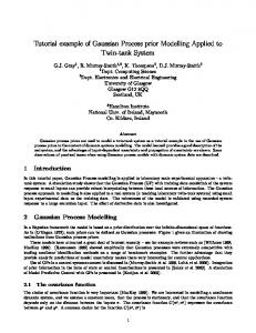
B. Dynamical system identification The identification method above was originally used for identification of static functions, but it can be extended to model dynamical systems as well [8]. Our task is to model the dynamical system (1) and be able to make n-step ahead prediction. One way to do nstep ahead prediction is to make iterative one-step ahead predictions up to desired step n whilst feeding back the predicted output. Two approaches to iterated one-step ahead prediction are possible using GP model. In the first approach only the mean values of the predicted output are feed back to input. Vector of regressors x(k) at time sample k from (2) for GP model is composed from L past predicted outputs and L past inputs: x(k) = [ˆ y (k − 1), . . . , yˆ(k − L), u(k − 1)), . . . , u(k − L)]T (11) where yˆ(k − i) and u(k − i) are past prediction yˆ and input u at time sample (k − i) respectively. This “naive” approach neglects information about the uncertainty of the output and is similar to that used in modelling dynamic systems with NNs. The obtained variance is still a rough indicator of the model’s local one-step ahead accuracy, but the values of predicted mean and variance are not correct for the n-step ahead prediction. C. Propagation of the uncertainty through the GP model In second approach to n-step ahead prediction not only the mean value of the predicted output is feed back to input of the GP model, but complete output distribution of the GP model is feed back instead [16], [12]. This way GP model not only models dynamical behaviour of the system but also provides the information about confidence in its prediction. Two realizations of this approach are possible: • numerical integration over input distribution, e.g. with MCMC method and • analytical solution, where assumption about output having Gaussian probability distribution, is made [12], [11]. Latter approach, referred to as “exact” approach, is depicted in Fig. 1. Output distribution N (m(k), v(k)) with mean value m(.) and variance v(.) of the model in time step k is presumed to be Gaussian. Note that distribution in Fig. 1 is denoted with N and not N , as it is Gaussian only by presumption. In “exact” approach input to GP model vector of past outputs xyˆ(k) = [ˆ y (k − 1), . . . , yˆ(k − L)]T is presented as:
-1
Z Z
... -L
u (k -2 )
G a u s s ia n p ro c e s s m o d e l
u (k -L )
N ( m ( k ) ,v ( k ) )
...
N N N
( m ( k - 1 ) ,v ( k - 1 ) )
-1
Z
-2
( m ( k - 2 ) ,v ( k - 2 ) )
Z
( m ( k - L ) ,v ( k - L ) )
Z
... -L
Fig. 1. Simulation with repeated one step-ahead prediction of dynamical model where uncertainty is propagated
The regressor x from (11) is completed with vector xu = [u(k − 1)), . . . , u(k − L)]T , where u(k − i) is the value of the input at time sample k −i. As they are known precisely, we can view on each of these values as on distribution with variance σ 2 (u(k − i)) = 0. Thus the input of the GP model x, at which we wish to predict the output, is a normally distributed random variable with mean vector µ x and covariance matrix Σ x : µ· ¸ · ¸¶ µ yˆ Σ yˆ 0 µx , Σ x ) = N x ∼ N (µ , (15) xu 0 0 New output yˆ(k) ∼ N (m(x(k)), v(x(k)) + v0 ) at time sample k is computed using (16) and (17), see [11], [12] for details. µx , Σ x ) = Ex [µ(x)] m(µ (16) 2 2 2 µx , Σ x ) = Ex [σ (x)] + Ex [µ(x) ] − (Ex [µ(x)]) (17) v(µ R +∞ µx , Σ x ) dx and the exwhere Ex [f (x)] = −∞ f (x) p(x|µ pressions for mean µ(x) and variance σ(x) are from (9) and (10) respectively. Due to space limitation only final expressions for mean and variance are given, refer to [12] for detailed calculations. Predicted mean m(.) and predicted variance v(.) at time sample k for normally distributed random variable x with mean vector µ x and covariance matrix Σ x are: µx , Σ x ) = m(µ
N X
µx , xi ) Ccorr1 (µ µ x , xi ) βi C(µ
(18)
i=1
and µyˆ, Σ yˆ) xyˆ(k) ∼ N (µ
(12)
where the vector of mean past predictions µ yˆ is µ yˆ = [m (xyˆ(k − 1)) . . . m (xyˆ(k − L))]T
(13)
and elements Σi,j of covariance matrix Σ yˆ between past predicted outputs are ½ v(xyˆ(k − i)) + v0 , i=j Σi,j = (14) cov (ˆ y (k − i), yˆ(k − j)) otherwise.
µx , Σ x ) = v − m(µ µx , Σ x )2 − v(µ N X ¡ −1 ¢ µx , xi )C(µ µx , xj )Ccorr2 (µ µx , xb ) (19) − Kij − βi βj C(µ i,j=1
where
¯ ¯−1/2 µx , xi ) = ¯ I + W−1Σ x ¯ Ccorr1 (µ · ¸ 1 µx − xi )T ∆−1 (µ µx − xi ) (20) exp (µ 2
B. Operating region, measurements and results
−1
∆−1 = W−1 − (W + Σ x )
(21)
¯ ¯ µx , xb ) = ¯ 2W−1Σ x + I¯ Ccorr2 (µ · ¸ 1 T −1 µx − xb ) Λ (µ µx − xb ) (22) exp (µ 2 µ ¶−1 µ ¶−1 1 1 Λ−1 = W W + Σx − (23) 2 2
The represented second order system is single-input single-output system, where voltage U on the DC motor of pump P 1 is the input and liquid level h2 in tank R2 is the output of the system. Static characteristic of the system’s response is given in Fig. 3. Besides the static nonlinearity, observed in Fig. 3, the system’s dynamics is nonlinear too. Statical characteristic of the chosen subsystem of the plant 60
and xi and xj are i-th and j-th input regressors with their mean xb = 12 (xi + xj ), β = K−1 y, I is D × D identity matrix and W−1 is diagonal matrix of hyperparameters wi : W−1 = diag[w1 , . . . , wD ].
50
level h2 (cm)
40
IV. I DENTIFICATION OF A TWO TANK SYSTEM A. Laboratory pilot plant and chosen subsection for identification The process scheme of laboratory pilot plant’s subsystem is presented in Fig. 2. Subsystem consist of two tanks, R1 and R2, connected with flow paths, which serve to supply liquid from the reservoir R0.
30
20
10
0 0.5
Fig. 3. R1
LT 2
1.5
2
2.5 voltage U (V)
3
3.5
4
4.5
Static characteristic of the chosen subsystem of the plant
R2
R0
P1
V5
Fig. 2.
1
Process scheme of chosen subsystem of the plant
Flow path from reservoir R0 to tank R1 has built-in pump P 1, driven with DC motor with permanent magnet. The angular speed of the motor is controlled by the analog controller. The time constant of the angular speed is very short compared to the time constants of the dynamics of the levels in the tanks, i.e. we can consider no lag between the reference speed and the real one. Flow is generated by varying the angular speed of the pump P 1. The other interesting part is manual valve V 5, which is positioned on the path from tank R2 to reservoir R0. It is partly open, so it enables liquid flow from tank R2 back to reservoir R0. Capacity of the reservoir R0 is much greater than capacity of the tanks so that its level can be considered constant during the operation. Voltage on the motor, which represents the input into the system, drives the pump P 1. Pump generates flow from reservoir R0 to tank R1. Liquid flows from tank R1 to tank R2 and from there back to reservoir R0 through ventil V 5. The liquid level in tank R2 represents the output of the system.
Working region is restricted with height hmax = 60 centimeters of the tanks R1 and R2. The maximum voltage on P 1 was fixed to Umax = 4 Volts with trial and error method, preventing the liquid level h1 to reach the top hmax of the tank R1. Sample time Ts = 10 seconds was chosen experimentally, so that dynamics of the system was satisfactory captured. Identification and validation data for GP model was obtained with measurements. Pseudo–random binary signal (PRBS) was used for input, except that the value of the magnitude of the signal could occupy any value between Umin = 0.8 and Umax = 4 Volts when changed. Two different signals were used, one for training of the model and one for model validation. The signal for training is depicted in Fig. 4 and the signal for validation in Fig. 5. The second order model was assumed as the underlying system is of second order too. Training points were sampled arbitrary from training signal. 92 training points were used for training of the GP model. The number of training points was selected as a tradeoff between quality of prediction and training time. As this is nonparametric model, where all training inputs are constituting the model via covariance matrix K, merely increasing the number of training points would not necessary substantially improve the prediction of the model, as is the case in our example. With the training the following values were gained for hyperparameters: v = 218, v0 = 0.03, w = [2.0E − 4, 2.5E − 3, 0.155, 1.28E − 2]T . The result of the simulation of the GP model without propagation of variance — the “naive” method — can be seen in Fig. 6 and the result of simulation with propagation of the variance — the “exact” method — in Fig. 7. From Fig. 6 we can deduce, that the mean value of the model’s
Gp model simulation on validation signal, order=2
Pilot plant training signal 24
voltage U (V)
6 utrain
mean−2σ mean+2σ predicted mean process
22
4
20 2
0
500
1000 time (s)
1500
2000
level h2 (cm)
25
level h2 (cm)
18 0
20
14 12
15
10
10 5 0
y 0
Fig. 4.
500
1000 time (s)
8 train
1500
6
2000
Training signal for LMGP model of the plant
valid
2
18 300 time (s)
400
500
600
25
level h2 (cm)
20
200
400
500
600
mean−2σ mean+2σ predicted mean process
22
3
100
300 time (s)
Validation of the GP model with simulation – “naive” method
u
0
200
24
4
1
100
Gp model simulation on validation signal with propagation, order=2
Pilot plant validation signal
voltage U (V)
0
Fig. 6.
5
level h2 (cm)
16
16 14 12
20
10
15 10
8
y
valid
5
6 0
100
200
300 time (s)
400
500
Fig. 5.
Validation signal for LMGP model of the plant
600
Fig. 7.
output corresponds quite well to target. The variance on the other hand can not be used as the proper measure of confidence, as it is not taking the uncertainty of the input into account, which results in too firm confidence in prediction. That is not the case when “exact” method is used. The confidence in the prediction loosens as the uncertainty of previous output is taken into consideration. This is particulary highlighted in the regions, modelled with smaller number of data, as can be seen from Fig. 8 in time interval from 400 to 550 seconds. We can observe, that during most of the simulation system’s output y lies within the 95% measure of confidence interval 2σ around the predicted output of the GP model yˆ: |ˆ y (t) − y(t)| < 2σ(t), see Fig. 8. Two quality measures [8] were used for results of validation: •
mean squared error (SE) SE = and
N 1 X 2 e N i=1 i
(24)
•
0
100
200
300 time (s)
400
500
600
Validation of the GP model with simulation – “exact” method
log-predictive density error (LD) [12] ¶ N µ 1 X e2i 2 LD = log(2π) + log(σi ) + 2 2N i=1 σi
(25)
where ei = yˆi − yi is error of model’s prediction and σi2 predicted variance of the model in i-th time step. Their evaluation for both simulation methods is given in Table I. It can be seen from comparison of SE, that the mean predicted value does not improve much with the use of “exact” method. More important is, that the variance can be used as the measure of confidence when using “exact” method, which can be seen from comparison of LD values in Table I and simulation results in Figs. 6, 7 and 8. TABLE I VALUES OF QUALITY MEASURES ON GP MODEL SIMULATION RESULTS method SE LD
“naive” 0.2039 1.66
“exact” 0.2019 0.65
Prediction error of the model and 95% confidence zone
ACKNOWLEDGMENT
1.8
The support of the Ministry of Higher Education, Science and Technology, Grant No. P2-0001, is gratefully acknowledged.
|eexact|
1.6
2 σnaive 2 σexact
1.4
level h2 (cm)
1.2 1
R EFERENCES
0.8
[1] 0.6
[2] 0.4 0.2 0
[3] 0
100
200
300 time (s)
400
500
600
Fig. 8. Absolute error of model with propagation compared to 95% confidence values of “naive” and “exact” method
V. C ONCLUSIONS In this paper the identification of dynamical systems with GP model is presented and used on two-tank system example. The identified GP model was validated with simulation. Two simulation methods were used — “naive” method without and “exact” method with propagation of variance. The main advantage of GP model over NN or fuzzy models is, that its output is predicted Gaussian distribution instead of predicted value. Gaussian distribution is defined with its mean and variance and in terms of GP model we can use the mean as prediction value and variance as the measure of confidence in prediction. It was shown that this uncertainty measure can be effectively used with “exact” realization to improve simulation results of the GP model. Second advantage of GP model over neural networks or fuzzy logic models is the smaller number of parameters that need to be optimized, as this reduces the problem of local minima. Another potential benefit of GP model is possibility to include prior knowledge in elegant matter. Disadvantage of the GP model is high computational burden, associated with training of hyperparameters and propagation of the uncertainty. In this paper two-tank system was successfully identified with nonparametric GP model. Only six hyperparameters of the model needed to be optimized. The model was validated with simulation, where gained uncertainty was effectively used to obtain confidence regions around predicted output. Ongoing activities include incorporation of prior knowledge into GP model and improvement of the algorithms as well as various applications of GP models.
[4] [5] [6] [7] [8]
[9]
[10] [11]
[12] [13] [14] [15] [16]
L. Ljung, System Identification – Theory for the User, 2nd Edn., Prentice Hall, New Jersey, 1999. J. Kocijan, R. Murray-Smith, C.E. Rasmussen and A. Girard, “Gasussian process model based predictive control”, Proc.: American Control Conference, Boston, pp. 2214-2219, 2004. E. Solak, R. Murray-Smith, W.E. Leithead, D.J. Leith and C.E. Rassmusen, “Derivative observations in Gaussian Process Models of Dynamic Systems”, S. Becker, S. Thrun and K. Obermayer (Eds) Advances in Neural Information Processing Systems 15, MIT Press, pp. 529–536, 2003. J. Kocijan and D.J. Leith, “Derivative Observations used in Predictive Control”. Proc.: Melecon 2004, Dubrovnik, 2004. A. O’Hagan, “On curve fitting and optimal design for regression (with discussion)”, Journal of the Royal Statistical Society B, vol. 40, pp.1-42, 1978. C.E. Rasmussen, Evaluation of Gaussian Processes and Other Methods for NonLinear Regresion, PhD thesis, University of Toronto, Toronto, 1996. R.M. Neal, Bayesian learning for neural networks, Springer Verlag, New York, 1996. J. Kocijan, A. Girard, B. Banko and R. Murray-Smith, “Dynamic Systems Identification with Gaussian Processes”, Proc.: 4th Mathmod, Wien, 2003, extended version in Mathematical and Computer Modelling of Dynamic Systems (in press). J. Kocijan, B. Banko, B. Likar, A. Girard, R. Murray-Smith and C.E. Rasmussen, “A case based comparison of identification with neural networks and Gaussian process models”, Proc.: IFAC Intelligent Control Systems and Signal Processing Conference, Faro, pp. 137– 142, 2003. G. Gregorˇciˇc and G. Lightbody: “Gaussian Processes for Modelling of Dynamic Non-linear Systems”, Proc.: Irish Signals and Systems Conference, Cork, 2002. A. Girard, C.E. Rasmussen, J. Qui˜nonero Candela and R. MurraySmith, “Multi-step ahead prediction for nonlinear dynamic sytems A Gaussian Process treatment with propagation of the uncertainty”, S. Becker, S. Thrun and K. Obermayer (Eds) Advances in Neural Information Processing Systems 15, MIT Press, pp. 1033–1040, 2003. A. Girard, Approximate Methods for Propagation of Uncertainty with Gaussian Process Models, Ph.D. Thesis, University of Glasgow, Glasgow, 2004. C.K.I. Williams, “Prediction with Gaussina processes: from linear regression and beyond”, M.I. Jordan (Ed) Learning and Inference in Graphical models, Kluwer Academic Press, pp. 599–621, 1998. M.N. Gibbs, Bayesian Gaussian Processes for Regression and Classification, Ph.D. Thesis, Cambridge University, Cambridge, 1997. D.J. Mackay, “Gaussian Processes”, Information theory, inference and learning algorithms, Cambridge University Press, 2003. J. Kocijan and A. Girard, “Incorporated linear local models in Gaussian process model”, accepted for presentation at 16th IFAC World Congress, Prague, 2005.