Patrick Dickinson, Koffi Appiah, Andrew Hunter and Stephen Ormston. Department of ... using non-visual sensors, and beyond the scope of our work. However, automated visual ..... on the RC300 [2], and operating at a clock speed of 25MHz. Video stream is .... DSP Algorithms,â www.accelchip.com, March 2005. [2] Celoxica ...
An FPGA-Based Infant Monitoring System Patrick Dickinson, Koffi Appiah, Andrew Hunter and Stephen Ormston Department of Computing and Informatics University of Lincoln Lincoln LN6 7TS, UK
Abstract
video stream
We have devised an automated visual surveillance system for monitoring sleeping infants. The system architecture requires that low-level image processing is executed on-camera by an embedded signal processing unit: we have designed and built this unit using a Xilinx’s Virtex II XC2v6000 FPGA. The processing unit quantifies the level of scene activity using a specifically designed background subtraction algorithm. In this paper we begin by describing the overall structure of our system. We proceed by presenting our algorithms, and demonstrating their effectiveness in measuring scene activity. We conclude by describing the FPGA-based low-level processing functions, and show how we have optimised them for maximum efficiency on this platform.
video stream
On-Camera Processing Unit
On-Camera Processing Unit
processed data
processed data
user selected video stream
video stream
On-Camera Processing Unit
processed data
Central Montoring Unit
Smart Camera Unit
Figure 1: System overview
less connections) to a single PC-based monitoring station. This enables a single carer may monitor several infants simultaneously. However, to support this hardware structure we need to adopt a corresponding distributed processing architecture. Video surveillance systems are typically characterised by hierarchical levels of processing. At the lowest-level, salient features of the scene, such as edges, regions, or motion information are extracted from raw video stream data: this stream occupies a high bandwidth such that processing requires the computational resources of a typical PC to achieve real-time performance. Thus, it is not feasible to process multiple video streams entirely on the monitoring station. Moreover concurrent wireless connections carry a limited shared bandwidth, which would restrict the transmission of multiple video stream signals. For this reason, low-level processing is to be implemented on-camera using an embedded FPGA unit, and the results transmitted to the monitoring station. The bandwidth requirement of the processed data is minimal, so that many cameras may simultaneously transmit results, whilst a raw video stream is transmitted from one (user selected) camera. We term the camera/embedded processor setup a “smart camera”. The overall system setup is shown graphically in figure 1.
1. Introduction Advances in surveillance technology have exposed many potential areas of application. Researchers have monitored human activity in various environments, with the aim of detecting specific modes of behaviour, such as criminal activity [11]. More recently, researchers such as Nait-Charif [7] have considered applying these technologies to supportive care, where automatic detection of hazardous events or behaviours can assist carers looking after vulnerable individuals. Thus far, infant monitoring has attracted little attention from vision researchers, however other monitoring technologies have been applied successfully. Qiaobing [8] used Hidden Markov Models to analyse infant cry signals and measures a level of distress. Sasanov [9] used an accelerometer to measure infants level of activity, and determine whether an infant is asleep or awake. Thus there is evidence that despite the apparently unpredictable nature of infant behavior, some level of analysis is possible. The objective of our work, then, is to develop automated visual surveillance technologies to support infant care. We have designed a surveillance system in which multiple cameras may be simultaneously connected (via wire1
1.1
System Functionality
1. The design of appropriate low and high-level processing algorithms.
PDSP provides system designers with the software components and development environment (such as C/C++ compilers) for rapid development across a broad breath of applications [10]. This allows designers the flexibility to refine algorithms late into the development cycle without significant impact on the development schedule. However, the demands of image processing systems outstrip the performance provided by the current generation PDSPs. This is because PDSPs are inherently sequential in nature, timesharing a restricted number of physical multipliers. This reduces the opportunity to fully parallelise processing algorithms [1] and ultimately limits data throughput. The FPGA platform offers rich resources, fast configuration speed, reconfigurability and support for extensive parallelism [6] making it an ideal choice for image processing. The suitability of this platform for low-level image processing has been demonstrated by a number of authors [13], [15]. In contrast to PDSPs, FPGAs are programmed by specifying the hardware functionality at register transfer level (RTL) using VHDL or verilog: consequently, image processing applications tend to suffer from longer development cycles, and sometime require re-synthesis, which may cause the FPGA to operate with reduced frequency [10]. However, the performance improvements offered by a highly parallel architecture are a deciding factor for our system. We chose to use a Xilinx Virtex II XC2v6000 FPGA for development, based on the appropriate computational and integrated memory resource offered by this platform. In the rest of this paper we describe our processing algorithms in more detail, and present an analysis of their effectiveness. This analysis is based on a PC-based prototype implementation. We then proceed to describe how we have re-engineered the algorithm for optimal implementation on the FPGA platform. We conclude with a performance comparison between the PC and FPGA based implementations, and a discussion of our work.
2. Implementation and assessment of these algorithms on PC platform.
2. Algorithm Design
Sleep phase is an appropriate context for remote monitoring. While awake, infants require direct supervision from a carer: during sleep, infants are mostly inactive and their movements constrained, such that the use of remote monitoring is feasible. The most severe hazards facing sleeping infants are acute medical conditions which are best detected using non-visual sensors, and beyond the scope of our work. However, automated visual monitoring may provide support for routine care. Sleeping infants normally experience a sleep-wake cycle in which they pass through different sleep modes (light/heavy) and wake naturally before returning to sleep. Infants sometimes wake for some other reason (such as hunger) which precipitates some action on the part of the carer (such as feeding). If left unattended in this state an infant typically develops a level of distress which impedes resolution of the situation. The aim of our system is to detect infant awakenings, and report those which are likely to require attention before distress develops. We propose to achieve this by quantifying the level of scene activity in terms of intensity and duration, and using these measurements to differentiate brief awakenings associated with the normal sleep-wake cycle from those which may require attention. Our system is user configurable, so that a carer may tune the sensitivity to match the behaviour of an individual infant.
1.2
Implementation and Platform Choice
Our work on developing the system so far comprises the following:
Our premis is that different perceived levels of activity (characterised by intensity and duration) are indicative of the waking state of the infant: short or low-intensity activity is assocaited with normal sleep-wake cycle and requires no attention. Longer or more agitated movement indicates that attention is required. The user may configure the system appropriately to match individual behaviour. Low-level processing is implemented on the FPGA, and estimates the level of activity from one frame to the next. High level processing models the activity level over time, and will be implemented on the PC-based monitoring station. There are some additional technical considerations that affect the design of our algorithm. Frames are captured by a camera observing the sleeping infant. Assuming that light-
3. Re-development of the low-level processing algorithm for FPGA platform. We have chosen to use a Field Programmable Gate Array (FPGA) platform over a Programmable Digital Signal Processor (PDSP) or embedded microprocessor to develop the smart camera processing unit. This choice has been guided by a number of considerations. Ma [6] characterises an ideal platform for developing image processing functions by flexibility, and by performance high computational throughput, low-power consumption, and small design area. In general, choice of platform involves making a trade off between these goals, but high data throughput is a critical requirement. 2
ing levels are low, we intend to use infra-red illumination to light the scene in a similar fashion to the low-light shooting mode available on many consumer DV camcorders. Under these conditions the captured frame image is monochromatic, and suffers from a significant level of noise.
2.1
new pixel value is classified as foreground equation 2 is still applied, but σ 2 is set to a default value. Applying equation 1 to each pixel results in a binary foreground image mask. To remove noise we apply morphological “erode” and “dilate”operations to the mask using a square 3 × 3 structuring element. We then calculate the proportion of foreground pixels in the mask, θ, which we define as the magnitude of activity for this frame. This value will be transmitted to the monitoring station for each frame.
Low-level Processing
We use a background subtraction algorithm to estimate of the intensity of activity between this frame and the previous frame. Background subtraction is a commonly used method of extracting foreground from video sequences. A model is maintained for each image pixel using the history of observed values, and some statistical process. Each pixel observation is classified as either foreground or background, based on it’s deviation from the current model, and is then used to update the background model. In this way, the model can adapt to slow lighting changes in the scene. Foreground pixels are thus taken to have been generated by a foreground process, such as a moving object. Many background subtraction algorithms have been proposed. The W4 system [4] models each pixel’s background using maximum and minimum observed values, and a maximum inter-frame difference. More sophisticated statistical have been introduced such as that used by the Wallflower system [14] which employs a per-pixel Weiner filter. A popular approach is to use a mixture of Gaussian model, such as that proposed by Stauffer [12] which can model multiple background processes for each pixel. We would like to employ Stauffer’s algorithm [12], however we are faced with some restrictions. Memory is limited, so we choose to model only one gaussian process per pixel. Secondly we use integer (fixed-point) arithmetic and avoid computationally complex mathematical functions, such as the exponent used in the Gaussian probability density function. Operating within these restrictions, we model each pixel’s background process as a mean intensity value µ, and a variance σ 2 . Note that these values are 1-dimensional, as pixel values are monochromatic. A pixel value is classified as background if the following holds: 2
(x − µ) ≤ kσ 2
2.2
The monitoring station maintains a history of activity Θ = {θn , . . . , θm } for each connected smart camera, where m is the last value received, (m − n) ≤ N , and N is the maximum number of values stored. Each value of θ is regarded as significant if it equals or exceeds some threshold θs . A corresponding set of values Γ = {γn , . . . , γm } is also maintained, and indicates the difference between the number of values of θ ≥ θs and the number of values of θ < θs during the preceding time period. When a new value θm+1 is received it is appended to Θ. A new value γm+1 is appended to Γ where γm+1 = γm + 1 if θm+1 ≥ θs or γm+1 = γm − 1 otherwise(γm+1 is restricted to be greater than 0). If (m − n) > N then the oldest values (θn ) and (tn ) are removed from the history. The monitoring station begins an alert state if the most recent value held in Γ reaches some threshold γs on this frame, and terminates the alert state if it drops below γs . The threshold values θs and γs are the user configurable parameters of the system. Note that for convenience we measure γs in seconds, rather than frames, to maintain framerate independence. This configurability allows the user to compensate for individual infant behaviour, and also for camera position and aspect.
3. Algorithm Evaluation We have evaluated the ability of our algorithm to discriminate between different perceived levels of activity. Our test data comprised 34 hours of video footage of sleeping infants. This was captured using a commercial DV camcorder operating in infra-red low-light mode. Three infants participated, and footage was captured in sections of 1 hour duration. We re-sampled most of the sequences from 25 Hz to 5 Hz to make storage more manageable. We manually inspected the data set, and made subjective assessment of each period of activity, recording the following information:
(1)
Where x is the new pixel value, and k is a constant which we set to 2.5. If the new pixel value is classified as background, the background model is updated as follows: µnew = αµ + (1 − α) x
(2)
2 = ασ 2 + (1 − α) x2 σnew
(3)
High-level Processing
1. start frame number 2. end frame number
2 Where α is a learning constant, and µnew and σnew are restricted to suitable minimum and maximum values. If the
3. Level of agitation (low, medium, high) 3
Ground Truth Parameter Set ψ = {40s, low, low} ψ = {40s, medium, medium} ψ = {16s, medium, medium} ψ = {16s, medium, medium} ψ = {6s, medium, medium} ψ = {1s, medium, medium}
4. Proportion of body involved (low, medium, high) The indexation scheme allows us to specify a subset of significant activites by defining a 3-dimensional parameter vector: ψ = {Dmin , Amin , Lmin },where Dmin in the minimum activity duration, Amin is the minimum perceived agitation, and Lmin is the minimum perceived localisation. Such a subset thus contains periods of footage representing a certain perceived minimum level of activity. We use Receiver Operator Characteristic (ROC) curves to quantify the evaluation [16]. ROC curves are an statistical analysis tool used to measure the effectiveness of a new parameterised classification test. Elements from a given data set are first pre-classified using a known “correct” test: the new test is then run over the data set, and the two classifications compared. Elements correctly classified as positive by the new test are “true positive”, and those correctly classified as negative are “true negative”. This is repeated for different values of the new test’s variable parameter: the resulting curved graph of sensitivity (true positives) against 1-specificity (true negatives) indicates the effectiveness of the test, and pinpoints an optimal parameter setting for the test. For our ROC curves, the parameter set ψ defines a subset of “ground-truth” positive events: other indexed periods of activity which are not selected by the parameter set represent negative events. The system has 2 configurable operational parameters, θs and γs , so we need to generate separate ROC curves against each. We use different ground truth sets of activities to evaluate these hypotheses. To generate an individual ROC curve we first decide which parameter to vary, and select an appropriate fixed value for the other. We then specify a set of ground truth positive events from our indexed data. For example, for one set of curves we varied θs , took γs = 10 seconds, and used a ground truth set defined by ψ = {16s, medium, medium}. Each ground truth event is compared with the system alert activation and deactivation times. If at least one alert temporally overlaps with a positive event, a “true positive” event is recorded, otherwise a “false negative” is recorded. If any alert overlaps with a negative event, a “false positive” is recorded, otherwise a “true negative” is recorded. We used several ground truth subsets for the evaluation. For each, we used ranges of values for the fixed parameter, generating sets of related ROC curves: the ground truth parameter sets, ψ, and corresponding varied parameter are summarised in table 1. Table 2 shows the fixed value parameters used for θs and γs .
3.1
Varied Parameter γs γs γs θs θs θs
Table 1: Ground truth parameter sets used for evaluation Varied θs γs
Fixed Parameter Values θs (%) = 7, 5, 3, 2, 1.5, 1.0, 0.7, 0.5, 0.2, 0 γs (s) = 0, 1, 5, 10, 15, 20, 30, 40, 60, 120, 180
Table 2: Fixed values for operational parameters used in evaluation the data set {16s, medium, medium}, with a fixed value of γs = 5s, the optimal value of θs is between 2 and 3% resulting in a sensitivity and specificity of about 0.8. However, it was noted that the system performed less well in some circumstances. Where we used a low fixed value of γs (eg 1 second) the system was typically unable to differentiate between different positive and negative ground truth events. This seems only to reflect the inappropriately large difference between γs and the minimum duration used to define ground truth positive events, resulting in the inability to discriminate by duration of activity. An example of such a curve is shown in figure 2(c). 1
1
0.9
0.9
0.8
0.8
0.7
0.7
0.6
0.6
0.5
0.5
0.4
0.4
0.3
0.3
0.2
0.2
0.1 0
0.1 0
0.2
0.4
0.6
0.8
1
0
0
0.2
(a)
0.6
0.8
1
0.6
0.8
1
(b)
1
1
0.9
0.9
0.8
0.8
0.7
0.7
0.6
0.6
0.5
0.5
0.4
0.4
0.3
0.3
0.2
0.2
0.1 0
0.4
0.1 0
0.2
0.4
(c)
0.6
0.8
1
0
0
0.2
0.4
(d)
Figure 2: Example ROC curves (a) ψ = 16s, medium, medium, γs = 5s (b) ψ = 40s, medium, medium, θs = 0.5% (c) a low fixed value of γs = 1s is used. (d) Low intensity activity in the ground truth.
Evaluation Results
Figure 2 (a) and (b) shows two example ROC curves. These curves are typical, and demonstrate the ability of the system to differentiate between different perceived levels of activity. As an example, we can estimate from 2 (a) that using
We encountered a more significant problem using the 4
ψ = {40s, low, low} data set. An example is shown in figure 2(d). In this case the system was unable to successfully discriminate between longer and shorter periods of low-level activity. This is because periods of low-intensity activity which are perceived to be continuous are processed by the system as a series of short activities. There are points in any such period where activity briefly stops, or falls to a very low level, causing the activity to be “broken-up” by the system. The result is that the system is unable to differentiate between what is perceived by the user as a series of short activities, and what is perceived as a longer continuous period: there is a lower-level of granularity in perception and indexing than in processing. It should also be noted that although activities are indexed as isolated events, temporal proximity to other activities may effect the system response. This is not accounted for in the indexation scheme.
pipelined pixel processing, and parallel processing in more detail. We conclude with an performance comparison between the FPGA and PC implementations. Read/write Enable
Memory Access Control
Morphology RAM #1 (mean)
RAM #2 (variance)
Pixel Processor (4-stage pipeline)
RAM #3 (mean)
4. The FPGA Implementation The FPGA implementation of the low-level processing was developed using Handel-C [2] and its functional behaviour has been tested using the DK3 design suite and Xilinx ISE 7.1i place and Route (PAR) tool. The platform is composed of Xilinx’s Virtex II XC2v6000 FPGA, 4 banks (36-bit addressable) of external SRAM totaling 32MByte packaged on the RC300 [2], and operating at a clock speed of 25MHz. Video stream is input to the board using a consumer DV camcorder (720×576 PAL), and a VGA image of the foreground pixel mask is output from the board for testing purposes. Starting with the prototype PC based implementation (written in C) we have re-engineered the processing to take advantage of the parallelisation and pipelining capabilities of the platform. We have optimised for speed, and achieved a throughput of one complete pixel process per clock cycle. By doing this we have also saved memory resources as we do not need to buffer output from the camera: we can process pixel values from the camera as quickly as they are received. The overall structure of the processing is shown in figure 3. Each RGB pixel value from the camera passes through a conversion stage to produce a 32-bit greyscale value. Simultaneously, the camera output address the corresponding statistical data in SRAM. The pixel value and statistics are simultaneously at the pipelined pixel processing unit. During processing, the new pixel statistics are written back to SRAM, and a 1-bit value corresponding to the background state of the pixel is output for morphological operations. The final result is output to a VGA monitor for testing purposes. Images are captured and processed in standard PAL (720×576) format. The VGA output resolution is 640×480, and images are cropped to this size during the morphological processing stage. In the rest of this section we describe the main features of memory structure,
Address Bus
RAM #4 (variance)
Pixel Data
32 Bit Fixed Point Converter
RGB to GreyScale Converter
Figure 3: System overview
4.1
Memory Useage
Memory resources have been identified as a performance constraint by other researchers [5]. In particular, the use of external memory is a limiting factor on clock rate [3]. We encountered the same problem with our system, in that the memory requirements of our algorithm exceed that available as BlockRAM: we were therefore forced to utilise the 4 available banks of external SRAM to store the statistics (µ and σ 2 ) for each pixel. These banks are single port, so that a bank may be either read or written on each clock cycle. To optimise processing speed we double buffer the statistics by organising the 4 banks into 2 pairs of switchable banks. On any particular clock cycle, one pair holds the current read values, and the other is used to store the new values for the next frame. The banks are switched each frame by a memory controller. The actual storage requirement for all values of µ and σ 2 is considerably less than the two 8 MByte blocks of SRAM used, as shown in table 3. Although this structure is wasteful in terms of storage resource useage, it enables us to achieve a much higher throughput. The memory space 5
Memory Block(s) RAM 1 and 3 (µ) RAM 2 and 4 (σ 2 )
Available (MBytes) 8 8
Used (MBytes) 1.17 1.17
Resource Flip Flops 4 input LUTs Block RAMs bonded IOBs GCLKs DCMs Occupied Slices
Table 3: SRAM memory useage Stage 1
Operations Compute ((x − µ) in equation 1. Compute µnew in equation 2. 2
2
Compute ((x − µ) in equation 1. Compute kσ 2 in equation 1.
3
Apply equation 1 using results from stage 2 and write result to BlockRAM. Apply equation 3, or reset σ 2 accordingly.
4
Cap σ 2 to maximum or minimum value.
output to a VGA monitor for testing. The result of operational structure is that the throughput is maximised at the expense of a slightly altered functionality: the result of the morphology is not used to select the update equations 2, and 3. Consequently the statistical model is more sensitive to image noise, although the perceived difference in operation from the PC version is negligible under normal noise levels.
4.4
Parallel Processing
We exploit the parallel processing architecture available on FPGA to run the different processing stages concurrently. This is emphasised by the logical processing block arrangement in 3. Pixel values from the camera are converted through the “RGB to Grayscale” converter, output from which is passed direcly into the “32 bit fixed point converter”. These two processors run in parallel, with a one cycle latency. Memory addressing and fetching from SRAM occurs simultaneously such that the corresponding pixel value and statistics are available simultaneously at stage 1 of the pixel processor. Morphological operations are also conducted in parallel with the pixel processor, such that the latency of the entire processing from pixel capture to completion of pixel processing is 8 cycles, with a further 14 cycles until the VGA display is updated.
required for morphological operations (erode and dilate) is only 1 bit per pixel, and we able to store the 3 buffers required for this in BlockRAM.
Pipelined Pixel Processing
The foreground mask and statistical update given by equations 1, 2, and 3 is executed by a four stage pixel processing pipeline. Table 4 summarises the operations at each stage. The current values of µ and σ 2 and the new pixel value (x) are input into the pipeline. On completion of stage four, the new values of µ and σ 2 are written to the appropriate location in SRAM. This pipeline enables us to concurrently process four pixels in four stages, resulting in a 1 pixel-percycle throughput.
4.5 4.3
Percentage 2% 4% 39% 41% 25% 8% 7%
Table 5: FPGA resource utilization
Table 4: Pixel Processing Pipeline
4.2
Total Used 1,821 out of 67,584 3,286 out of 67,584 57 out of 144 346 out of 824 4 out of 16 1 out of 12 2,567 out of 33,792
Morphology
Resource Useage and Performance
We have already reported the use of external SRAM resources in table 3. Overall FPGA resource use is described in table 5, using device xcv6000, package ff1152 and speed garde -4. To test speed performance we compared the FPGA implementation with the original corresponding code in the PC prototype. The PC code was developed using Borland C++ Builder 6, and compiled using the ’Release’ compile options for maximum speed. We measured the time taken to execute the low-level processing functions on PC and found an average time of around 40ms (25Hz). Coincidentally, this corresponds to the capture rate of the camera, so that
In order to achieve an optimal pixel-per-cycle throughput, we have modified the original PC algorithm slightly for FPGA implementation. Originally noise removal was executed by erode and dilate operations prior to updating the pixel statistics. However, we have re-designed this stage to run concurrently with the pixel pipeline. The result of applying equation 1 in stage 3 of the pipeline is stored in a 307200 bit buffer in BlockRAM. Erosion is applied to this buffer, the results being stored in a second buffer of the same size. Dilation is applied to the second buffer, the results being stored in a third. The third buffer is used as 6
our PC implementation is just capable of real-time performance. The FPGA system is synchronized directly to the input camera, and therefore operates at a fixed rate of 25Hz. However, performance analysis indicates that much higher execution speeds are achieveable. Currently, it takes 8 clock cycles to process a pixel from capture until the morphology stage, and a further 14 clock cycles to output to the VGA display. Since our processing is optimally pipelined we process 1 pixel per clock cycle, which at a clock speed of 25MHz corresponds to a total time of 16.6ms (60Hz). In addition, analysis by the PAR tool indicates that the processing would be capable of running at a high clock speed, given appropriate external memory units. Hence our FPGA system is capable of achieving a significant improvement over our PC version.
[4] I. Haritaoglu, D. Harwood, L. Davis, “W4: Who? When? Where? What? a real-time system for detecting and tracking people,” Proc. IEEE International Conference on Automatic Face and Gesture Recognition, pp.222-227, 1998. [5] K. Johnston, D. Gribbon, and D. Bailey, “Implementing Image Processing Algorithms on FPGAs,” Proc. of the Eleventh Electronics New Zealand Conference, pp. 118-123, 2004. [6] J. Ma, “Signal and Image Processing Via Reconfigurable Computing,” Workshop on Information and Systems Technology, University of New Orleans, May 2003. [7] H. Nait-Charif, S. McKenna, “Activity summarisation and fall detection in a supportive home environment”, Proc. of IEEE International Conference in Pattern Recognition, vol. 4, pp. 323-326, 2004. [8] X. Qiaobing, R. Ward, C. Laszlo, “Automatic assessment of infants’ levels-of-distress from the cry signals,” IEEE Transactions on Speech and Audio Processing, vol 4, issue 4, pp. 253-265, July 1996.
5. Summary and Conclusions We have presented an overall design for our infant monitoring system, and described our processing algorithms. We have used a significant data set and statistical analysis to shown these algorithms to be effective in differentiating between perceived levels of infant. We have also implemented the low-level image processing functions on an FPGA as the basis for development of the smart camera component of our system. The features of this platform have enabled us to make various applicationspecific processing optimisations which have improved the computational performance of our system. Specifically, we have utilised a 4-stage pixel processing pipeline which allows us to increase data throughput and minimise storage of frame data. Comparing this platform to a contemporary PC platform has shown around a 2.5× speed improvement.
[9] E. Sasanov, N. Sasanova, S. Schukers, M. Neuman, CHIME study group 2004, ”Activity based sleep-wake identification in infants,” Physiological Measurement, vol. 25, no. 5, pp. 1291-1304(14), October 2004. [10] N. Sheshan, “DSPs vs. FPGAs in Signal Processing System Design,” Texas Instruments TM320C6000 DSPs, 2004. [11] A. Datta, M. Shah, N. Da Vittoria Lobbo, “Person-on-person violence detection in video data,” Proc. of IEEE International Conference in Pattern Recognition, vol 1, pp. 433-438, 2002. [12] C. Stauffer and W. Grimson, “Adaptive Background Mixture Models for Real-Time Tracking,” Proc. of IEEE Conference on Computer Vision and Pattern Recognition, pp. 246-252, 1999. [13] C. Torres-Huitzil, M. Arias-Estrada, “An FPGA Architecture for High Speed Edge and Corner Detection,” Proc. IEEE International Workshop on Computer Architectures for Machine Perception, pp. 112-118, 2000.
Acknowledgments This work was supported by an EPSRC CASE studentship in conjunction with Nectar Electronics Ltd, Durham, UK.
[14] K. Toyama K, J. Krumm, B. Brumitt, and B. Meyers, “Wallflower: Principles and practice of background maintenance,” Proc. IEEE International Conference on Computer Vision, pp. 255-261, 1999.
References
[15] G. Wall, F. Iqbal, J. Issac, X. Liu, and S. Foo, “Real time texture classification using field programmable gate arrays,” Proc. of IEEE Applied Imagery Pattern Recognition Workshop, pp. 133-135, 2004.
[1] AccelChip, Inc. “Comparison of Methods for Implementing DSP Algorithms,” www.accelchip.com, March 2005. [2] Celoxica, “Video and Imaging solution,” www.celoxica.com, 2004.
[16] MH. Zweig, G. Campbell, “Receiver-operating characteristic (ROC) plots: a fundamental evaluation tool in clinical medicine,” Clinical Chemistry, vol. 39, issue 4, pp.561-577, 1993.
[3] F. Crowe, A. Daly, T. Kerins, and W. Marnane, “Design of an Efficient Interface between an FPGA and External Memory,” Proc. IEE Irish Signals and Systems Conference, pp. 118-123, 2004.
7