An Improved Approximation Scheme for Scheduling a Maintenance and Under Linear. Deteriorating Jobs. Journal of Industrial and Management Optimization ...
AN IMPROVED APPROXIMATION SCHEME FOR SCHEDULING A MAINTENANCE AND PROPORTIONAL DETERIORATING JOBS ∗ Imed Kacem, Eugene Levner ∗
P lea s e cite th is p a p er a s fo llow s:
I. K a cem , E . L ev n er. A n Im p rove d A p p rox im a tio n S ch em e fo r S ch ed u lin g a M a inten a n ce a n d U n d er L in ea r D eterio ra tin g J o b s. J o u rn a l o f In d u stria l a n d M a n a g em ent O p tim iza tio n (Wo S , IF = 0 .8 4 ), 2 0 1 6 , Vo lu m e 1 2 , N umb er 3, pp: 811 - 817
Abstract In this paper, we re-visit the problem of scheduling a set of proportional deteriorating non-resumable jobs on a single machine subject to maintenance. The maintenance has to be started prior to a given deadline. The jobs as well as the maintenance are to be scheduled so that to minimize the total completion time. For this problem we propose a new dynamic programming algorithm and a faster fully polynomial time approximation scheme improving a recent result by Luo and Chen [JIMO (2012), 8:2, 271-283].
************** Classification. 2010 Mathematics Subject Classification. Primary: 90B35; Secondary: 90C59. Key words and phrases. Scheduling; deteriorating jobs; total completion time; maintenance activities; approximation scheme. Manuscript information. Received August 2013; revised December 2013 and March 2014.
1
1
Introduction
This paper deals with a single-machine scheduling problem with deteriorating jobs and non-availability constraints. The objective is to minimize the total completion time.
1.1
Problem statement
For the sake of convenience, we use the same notation as in [8]. We have a set of n proportional deteriorating non-resumable jobs J = {J1 , . . . , Jn }, all of which are available at time t0 > 0. For every job Jj , we denote the processing time by pj , and the completion time by Cj . The processing time pj of job Jj is defined by relation pj = αj sj , where αj > 0 and sj denote, respectively, the deteriorating rate and the starting time of job Jj . Moreover, we have to start a maintenance job of duration d before a given deadline s (s ≥ t0 ). Without loss of generality, we consider that jobs are sorted in Smallest Deteriorating Rate (SDR) order, i.e., α1 ≤ α2 ≤ ... ≤ αn . Indeed, it is easy to verify by the interchange argument that in any optimal solution the jobs scheduled before and those after the maintenance must respect this order. Moreover, we assume that jobs cannot fit all together before s (i.e., we have that t0 (1 + αj ) > s) and that every job Jj can be inserted before j=1,...,n
the maintenance (i.e., t0 (1 + αj ) ≤ s). We also assume that all the data (the deteriorating rates, the deadlines, and the maintenance duration) are integers. The problem is to schedule all deteriorating jobs and the maintenance on a single machine with the aim of minimizing the total completion time. According to [6], we denote the problem as 1|M (s, d), pj = αj sj | Cj . A j
close variant, where the maintenance starting time is fixed (i.e., equal to s), is denoted as 1|nr − a, pj = αj sj | Cj . j
1.2
Previous results
Several variations of the considered scheduling problems have been widely studied in the literature. For instance, Lee [7] has studied the problem version without the deterioration, taking only the non-availability interval into account. On the other hand, Gawiejnowicz and Kononov [3] have thorougly studied the scheduling problems for deteriorating jobs without the unavailability constraints. The most recent discussion of scheduling problems with 2
deteriorating jobs is given in Gawiejnowicz [2]. A possible combination of both variations has been addressed recently by Wu and Lee [11], Ji et al. [5], and Luo and Chen [8]. The NP-completeness of a decision version of the problem formulated by Wu and Lee [11] is proved by Gawiejnowicz [2]. A complete review of related works including various models and solution algorithms can be found in the cited papers. Luo and Chen [8] have successfully proved the existence of a fully polynomial time approximation scheme (FPTAS) for 1|M (s, d), pj = αj sj | Cj . j
(Recall that an FPTAS may be considered as the best possible approximation result for an NP-hard problem, see, for instance, Gens and Levner [4], and Woeginger [10]). Luo and Chen’s scheme is based on the consideration of a finite set of problems 1|nr − a, pj = αj sj | Cj , where the maintenance j
starts at some possible point. A dynamic programming algorithm and an FPTAS were proposed for the 1|nr − a, pj = αj sj | Cj and then exploited j
to solve the 1|M (s, d), pj = αj sj |
Cj problem. j
The time complexity of their FPTAS is O(n6 (ln D)4 /ε4 ) time, where D = max{s, d, 1 + αj , j = 1, . . . , n} and ε is the guaranteed relative error (0 < ε < 1). For completeness of exposition, it is worthy to mention that Ocetkiewicz [9] and Kellerer et al. [6] proposed different FPTAS versions for several other scheduling problems with deteriorating jobs.
1.3
Our contribution
By introducing a new (and simpler) dynamic programming formulation for the 1|M (s, d), pj = αj sj | Cj , and then converting it to a fully polynomial j
scheme, we derive a faster FPTAS of O(n6 (ln D)3 /ε3 ) time. We solve the problem without considering a set of the 1|nr − a, pj = αj sj | Cj problems j
which leads to a gain of O((ln D)/ε) time. The remainder of the paper is organized as follows. In Section 2, we propose a new dynamic programming algorithm. In Section 3, the new FPTAS is described and the complexity proof is presented. Finally, Section 4 provides some concluding remarks, possible extensions and perspectives.
3
2
Dynamic programming algorithm
The problem 1|M (s, d), pj = αj sj |
Cj can be optimally solved by applying j
the following dynamic programming algorithm A. This algorithm generates at every iteration j (j = 1, . . . , n) a set Ej composed of several states. Each state [t, w, f ] in Ej can be associated to a feasible partial schedule for the first j jobs. Variable t denotes the completion time of the last job scheduled before s and f is the total completion time of the associated partial schedule. Variable w is an auxiliary variable which is equal to j∈B Cj /(t + d) = j∈B
(1 + αi ) , where B is the subset of jobs scheduled after i∈{1,2,..,j}∩B
the maintenance in the associated partial schedule. Notice that Cj in w is the completion time of a job Jj in a subset of jobs B scheduled after the maintenance. We also define zj equal to (1 + αk ). This algorithm k=1,2,..,j
can be described as follows: ALGORITHM A (i) E1 = {[t0 (1 + α1 ) , 0, t0 (1 + α1 )], [t0 , (1 + α1 ) , (t0 + d) (1 + α1 )]} (ii) For j ∈ {2, 3, . . . , n} do: Ej =Ø. For every state [t, w, f ] in Ej−1 do: 1. Put [t, w + zj /(t/t0 ), f + (t + d)zj /(t/t0 )] in Ej 2. If t (1 + αj ) ≤ s then put [t (1 + αj ) , w, f + t (1 + αj ) + wtαj ] in Ej End For Remove Ej−1 End For (iii) Return OP T = min[t,w,f ]∈En {f }. Obviously, the set E1 consists of two partial schedules, in the first of which job J1 is placed before the maintenance, and in the second schedule job J1 is performed after the maintenance. As depicted in Figure 1, for every state [t, w, f ] in Ej−1 , job Jj has two possible positions in Ej , due to the SDR 4
rule dominance. The first possible position is the last position in the partial schedule, and job Jj completes in this case at time (t + d)zj /(t/t0 ) (This property immediately follows from the definitions of zj and t). The second possible position is the one just before the maintenance: Jj starts at time t if t (1 + αj ) ≤ s. The use of the second position implies that the processing times of the jobs scheduled after the maintenance will increase, which leads to an additional term in the total completion time, equal to wtαj . Let F and W be the upper bounds for the values f and w, respectively. If we add the restriction that, for every state [t, w, f ], the relations f ≤ F and w ≤ W must hold, then the running time of Algorithm A can be bounded by nF W s/t0 (by keeping only one vector for each state). Moreover, this complexity can be reduced to O(nW s/t0 ) by choosing at each iteration, for every pair (t, w), the state [t, w, f] with the smallest value of f . In the remainder of the paper, Algorithm A denotes the version of the dynamic programming algorithm in which we can take W = (1 + 1/αn ) (1 + αn)n and F = (t0 + d) (1 + 1/αn ) (1 + αn )n . Indeed, notice that F ≤ (t0 + d) W and W ≤ (1 + αn ) + (1 + αn )2 + ... + (1 + αn )n . These upper bounds stem from a schedule in which all the jobs are scheduled after the maintenance interval.
3
An improved FPTAS
The FPTAS below is based on the modification of the previous dynamic programming procedure (Algorithm A). It works by eliminating at every iteration some special states without altering significantly the final solution quality. We use a modification of dynamic programming technique which is close to that proposed by Woeginger [10]. The main idea of our FPTAS consists in a careful choice of the interval bounds and parameters F and W as well as the links between them in the recursive scheme defined below. Notice that, in contrast to the one-sided bounding of variable t exploited by Woeginger [10], we provide an upper bound and a lower bound for every approximate value of variable t in the generated states (see Lemma 1 below), which leads to a reduced time complexity. The improved scheme can be described as follows. Given an arbitrary ε > 0, we define θ = (1 + ε)1/n . Then, we split the state intervals as follows: Ir where R = ⌈ln(s/t0 )/ ln(θ)⌉ and Ir = [t0 θr−1 , t0 θr ] for
• [t0 , s] = r=1,...,R
5
Figure 1: Illustration of the dynamic programming algorithm A every r = 1, ..., R − 1 and IR = [t0 θ R−1 , s]. Up where P = ⌈ln(W )/ ln(θ)⌉ and Up = [θ p−1 , θp ] for
• [0, W ] = p=1,...,P
every p = 1, ..., P − 1, U0 = [0, 1] and UP = [θP −1 , W ]. Vm where M = ⌈ln(F )/ ln(θ)⌉ and Vm = [θ m−1 , θm ] for
• [0, F ] = m=1,...,M
every m = 1, ..., M − 1, V0 = [0, 1] and VM = [θM−1 , F ]. Our FPTAS A(ε) generates reduced sets Ej,⋄ instead of sets Ej . It can be described as follows: 6
ALGORITHM A(ε) (i) E1,⋄ = {[t0 (1 + α1 ) , 0, t0 (1 + α1 )], [t0 , (1 + α1 ) , (t0 + d) (1 + α1 )]} (ii) For j ∈ {2, 3, . . . , n} do: Ej,⋄ =Ø. For every state [t, w, f ] in Ej−1,⋄ do: 1. Put [t, w + zj /(t/t0 ), f + (t + d)zj /(t/t0 )] in Ej,⋄ 2. If t (1 + αj ) ≤ s then put [t (1 + αj ) , w, f + t (1 + αj ) + wtαj ] in Ej,⋄ End For Let [t, w, f ]r,p,m be the state in Ej,⋄ such that w ∈ Up and f ∈ Vm with the smallest possible t (ties are broken by choosing the state of the smallest f ). Set Ej,⋄ = {[t, w, f]r,p,m |r = 1, ..., R, p = 0, ..., P, m = 0, ..., M }. Remove Ej−1,⋄ End For (iii) Return min[t,w,f ]∈En,⋄ {f }. The first observation is that Algorithm A(ε) can be implemented in O(nRP M ) = O(n6 ln(D)3 /ε3 ) time. Indeed, at every iteration j we keep at most a single state in Ej,⋄ from every “box” Ir × Up × Vm (r = 1, ..., R, p = 0, ..., P, m = 0, ..., M). Furthermore, taking into account the property that ln(1 + ε) = O(ε) for sufficiently small ε > 0, from the definitions of the ceiling function and D, we can deduce that R = O((n/ε) ln(D)), P = O((n2 /ε) ln(D)) and M = O((n2 /ε) ln(D)). The analysis of the algorithm accuracy is based on the comparison of the states in Ej and Ej,⋄ . Lemma 1 For every state [t, w, f] ∈ Ej , there exists at least one state [t⋄ , w⋄ , f⋄ ] ∈ Ej,⋄ such that t/θ j ≤ t⋄ ≤ t, w⋄ ≤ θ j w and f⋄ ≤ θj f.
7
Proof. By induction. For j = 1, we can state that the lemma is true for every state since E1 = E1,⋄ . Let j ≥ 2. Assume that the result holds for levels 1, 2, ..., j − 1. We prove it for level j. Let [t, w, f ] be a state in Ej . Two cases are possible: Case 1: [t, w, f ] = [t′ , w′ +zj /(t′ /t0 ), f ′ +(t′ +d)zj /(t′ /t0 )] where [t′ , w′ , f ′ ] in Ej−1 . By induction, we know that there exists at least one state [t′⋄ , w⋄′ , f⋄′ ] ∈ Ej−1,⋄ such that t′ /θj−1 ≤ t′⋄ ≤ t′ , w⋄′ ≤ θj−1 w′ and f⋄′ ≤ θj−1 f ′ . By our construction, the state µ = [t′⋄ , w⋄′ +zj /(t′⋄ /t0 ), f⋄′ +(t′⋄ +d)zj /(t′⋄ /t0 )] is generated at iteration j but it can be replaced by another state, µ0 = [µ1,⋄ , µ2,⋄ , µ3,⋄ ], kept in Ej,⋄ where t′⋄ /θ ≤ µ1,⋄ ≤ t′⋄ , µ2,⋄ ≤ θ (w⋄′ + zj /(t′⋄ /t0 )) and µ3,⋄ ≤ θ (f⋄′ + (t′⋄ + d)zj /(t′⋄ /t0 )). Then, relations t/θj = t′ /θj ≤ µ1,⋄ ≤ t′ = t, µ2,⋄ ≤ θ θj−1 w′ + zj /( t′ /θj−1 /t0 ) = θj w and µ3,⋄ ≤ θ(θj−1 f ′ + (t′ + d)zj /( t′ /θ j−1 /t0 )) = θj f hold. We conclude that state µ0 = [µ1,⋄ , µ2,⋄ , µ3,⋄ ] verifies the required conditions. Case 2: [t, w, f ] = [t′ (1 + αj ) , w′ , f ′ +t′ (1 + αj )+w′ t′ αj ] where [t′ , w′ , f ′ ] in Ej−1 . By induction, we know that there exists at least a state [t′⋄ , w⋄′ , f⋄′ ] ∈ Ej−1,⋄ such that t′ /θj−1 ≤ t′⋄ ≤ t′ , w⋄′ ≤ θj−1 w′ and f⋄′ ≤ θj−1 f ′ . By construction, the state γ = [t′⋄ (1 + αj ) , w⋄′ , f⋄′ + t′⋄ (1 + αj ) + w⋄′ t′⋄ αj ] is generated at iteration j. Note that this state is feasible since t′⋄ (1 + αj ) ≤ t′ (1 + αj ) = t ≤ s. However, it can be replaced by another state γ 0 = [γ 1,⋄ , γ 2,⋄ , γ 3,⋄ ] kept in Ej,⋄ where t′⋄ (1 + αj ) /θ ≤ γ 1,⋄ ≤ t′⋄ (1 + αj ), γ 2,⋄ ≤ θw⋄′ and γ 3,⋄ ≤ θ (f⋄′ + t′⋄ (1 + αj ) + w⋄′ t′⋄ αj ). Then, relations t/θj = t′ (1 + αj ) /θ j ≤ γ 1,⋄ ≤ t′ (1 + αj ) = t, γ 2,⋄ ≤ θ θj−1 w′ = θj w and γ 3,⋄ ≤ θ θj−1 f ′ + t′ (1 + αj ) + θj−1 w ′ t′ αj ≤ θj f hold. We conclude that state γ 0 = [γ 1,⋄ , γ 2,⋄ , γ 3,⋄ ] verifies also the above relations. To conclude, in the both possible cases, we proved the existence of at least one state satisfying the lemma. Theorem 2 Algorithm A(ε) is an FPTAS for the 1|M (s, d), pj = αj sj [
Cj j
problem and it can be implemented in O (n6 ln(D)3 /ε3 ) time. Proof. Let [t∗ , w∗ , f ∗ ], be an optimal state in En . From Lemma 1, there exists a state [t⋄ , w⋄ , f⋄ ] ∈ En,⋄ such that f⋄ ≤ θn f ∗ = (1 + ε) f ∗ = (1 + ε) OP T . Note that [t⋄ , w⋄ , f⋄ ] is associated with a feasible complete schedule since [t⋄ , w⋄ , f⋄ ] ∈ En,⋄ . Moreover, this solution can be computed in a polynomial time in the input size and 1/ε.
8
4
Conclusions
In this note we considered the problem of minimizing the total completion time on a single machine where we have to schedule a set of proportional deteriorating non-resumable jobs under a maintenance constraint. For this problem we proposed an improved dynamic programming algorithm and a faster fully polynomial time approximation scheme (FPTAS) compared to the best existing result by Luo and Chen [8]. More precisely, by introducing a simpler dynamic programming formulation and then properly converting it, we obtained a faster FPTAS of O(n6 (ln D)3 /ε3 ) time, leading to a gain of O(ln(D)/ε) time. The gain can be especially sensitive in problems of maintenance management of high-precision manufacturing processes where the value of ln(D)/ε may be up to several hundred. The proposed techniques can be exploited for solving modifications and extensions of the considered scheduling problem. In particular, it is applicable for finding improved FPTASs for the problem of minimizing the makespan, 1|M(s, d), pj = αj sj | max {Cj }. As well, it can be used for solving the problem in which the maintenance duration depends on the set of jobs to be done before/after the maintenance, and a job’s deteriorating rate depends on whether it is processed before or after the maintenance. An interesting open question is: either to find a "strong FPTAS", whose complexity does not depend upon ln(D), or to prove that such an algorithm does not exist if P=NP.
5
Acknowledgements
The authors would like to thank Professor T.C.E. Cheng for interesting and beneficial discussions on the subject. They also express their acknowledgement to the anonymous referees and the editor, whose constructive comments helped improve the exposition of this paper. The research of the second author was supported in part by the National Natural Science Foundation of China under grant 71101016. The second author also thanks Prof. Peng-yu Yan for helpful discussions of the FPTAS methodology.
References [1] S. Gawiejnowicz, Scheduling deteriorating jobs subject to job or machine availability constraints, European Journal of Operational Research, 180 (2007), 472-478. 9
[2] S. Gawiejnowicz, Time-Dependent Scheduling, EATC Monograph in Theoretical Computer Science, Springer, 2008, 390 pp. [3] S. Gawiejnowicz and A. Kononov, Complexity and approximability of scheduling resumable proportionally deteriorating jobs, European Journal of Operational Research, 200 (2010), 305-308. [4] G. Gens and E. Levner, Fast approximation algorithm for job sequencing with deadlines, Discrete Applied Mathematics, 3 (1981), 313-318. [5] M. Ji, Y. He and T. C. E. Cheng, Scheduling linear deteriorating jobs with an availability constraint on a single machine, Theoretical Computer Science, 362 (2006), 115-126. [6] H. Kellerer, K. Rustogi, V.A. Strusevich, Approximation schemes for scheduling on a single machine subject to cumulative deterioration and maintenance, Journal of Scheduling, in press, DOI: 10.1007/s10951-0120287-8. [7] C.-Y. Lee, Machine scheduling with an availability constraint. Optimization applications in scheduling theory, Journal of Global Optimization, 9 (1996), 395-416. [8] W. Luo and L. Chen, Approximation schemes for scheduling a maintenance and linear deteriorating jobs, Journal of Industrial and Management Optimization, 8 (2012), 271-283. [9] K.M. Ocetkiewicz, A FPAS for minimizing total completion time ina single machine time-dependent scheduling problem, European Journal of Operational Research, 203 (2010), 316-320. [10] G. J. Woeginger, When does a dynamic programming formulation guarantee the existence of a fully polynomial time approximation scheme (FPTAS)?, INFORMS Journal on Computing, 12 (2000), 57-74. [11] C.-C.Wu and W.-C. Lee, Scheduling linear deteriorating jobs to minimize makespan with an unavailability constraint on a single machine, Information Processing Letters, 87 (2003), 89-93.
10