An Inferential Framework for Network Hypothesis Tests

An Inferential Framework for Network Hypothesis Tests: With Applications to Biological Networks

A dissertation submitted in partial fulfillment of the requirements for the degree of Doctor of Philosophy in Biostatistics at Virginia Commonwealth University.

by Phillip D. Yates

Nitai D. Mukhopadhyay, Director Edward L. Boone R. K. Elswick, Jr. Levent Dumenci Viswanathan Ramakrishnan

Virginia Commonwealth University Richmond, Virginia July, 2010

Copyright 2010, Phillip D. Yates All Rights Reserved

Abstract

AN INFERENTIAL FRAMEWORK FOR NETWORK HYPOTHESIS TESTS: WITH APPLICATIONS TO BIOLOGICAL NETWORKS By Phillip D. Yates, Ph.D. A dissertation submitted in partial fulfillment of the requirements for the degree of Doctor of Philosophy at Virginia Commonwealth University. Virginia Commonwealth University, 2010. Major Director: Nitai D. Mukhopadhyay, Assistant Professor, Department of Biostatistics The analysis of weighted co-expression gene sets is gaining momentum in systems biology. In addition to substantial research directed toward inferring co-expression networks on the basis of microarray/high-throughput sequencing data, inferential methods are being developed to compare gene networks across one or more phenotypes. Common gene set hypothesis testing procedures are mostly confined to comparing average gene/node transcription levels between one or more groups and make limited use of additional network features, e.g., edges induced by significant partial correlations. Ignoring the gene set architecture disregards relevant network topological comparisons and can result in familiar n ≪ p over-parameterized test issues. In this dissertation we propose a method for performing one- and two-sample hypothesis tests for (weighted) networks. We build on a measure of separation defined via a local neighborhood metric. This node-centered additive metric exploits the network properties of nearby neighbors. The use of local neighborhoods seeks to lessen the effect of a large number of (potentially) estimable parameters; biology or algorithms are commonly used to further reduce the prospect of spurious biological associations. Where possible, we avoid specifying dubious network probability models. In order to draw statistical inferences we use a resampling approach. Our method allows for both an overall network test and a post hoc examination of individual gene/node effects. We evaluate our approach using both simulated data and microarray data obtained from diabetes and ovarian cancer studies.

Contents

1 Introduction 1.1

1.2

1.3

1.4

1

Networks Are Everywhere . . . . . . . . . . . . . . . . . . . . . . . . . . . .

2

1.1.1

Physics . . . . . . . . . . . . . . . . . . . . . . . . . . . . . . . . . . .

4

1.1.2

Mathematics . . . . . . . . . . . . . . . . . . . . . . . . . . . . . . .

5

1.1.3

Scale-Free, Small-World Models . . . . . . . . . . . . . . . . . . . . .

6

1.1.4

Computer Science and Applications in Engineering . . . . . . . . . .

9

1.1.5

Trees . . . . . . . . . . . . . . . . . . . . . . . . . . . . . . . . . . . .

10

Social Networks . . . . . . . . . . . . . . . . . . . . . . . . . . . . . . . . . .

12

1.2.1

Descriptives and Estimation . . . . . . . . . . . . . . . . . . . . . . .

14

1.2.2

Clustering and Block Models . . . . . . . . . . . . . . . . . . . . . . .

20

Biological Networks . . . . . . . . . . . . . . . . . . . . . . . . . . . . . . . .

23

1.3.1

Motifs . . . . . . . . . . . . . . . . . . . . . . . . . . . . . . . . . . .

24

1.3.2

Protein Interaction Networks . . . . . . . . . . . . . . . . . . . . . .

28

1.3.3

Gene Networks . . . . . . . . . . . . . . . . . . . . . . . . . . . . . .

30

Modeling Biological Networks . . . . . . . . . . . . . . . . . . . . . . . . . .

32

iii

1.5

1.6

1.4.1

Of Mathematics and Machines . . . . . . . . . . . . . . . . . . . . . .

33

1.4.2

Correlation Networks . . . . . . . . . . . . . . . . . . . . . . . . . . .

35

1.4.3

Inferring Network Structure or Topology . . . . . . . . . . . . . . . .

36

1.4.4

Validating Models . . . . . . . . . . . . . . . . . . . . . . . . . . . . .

40

Comparing Networks . . . . . . . . . . . . . . . . . . . . . . . . . . . . . . .

44

1.5.1

Identifying H0 . . . . . . . . . . . . . . . . . . . . . . . . . . . . . . .

46

1.5.2

Isomorphisms and Deformations . . . . . . . . . . . . . . . . . . . . .

48

1.5.3

Topological Parameters . . . . . . . . . . . . . . . . . . . . . . . . . .

50

1.5.4

Sequence Alignment . . . . . . . . . . . . . . . . . . . . . . . . . . .

52

1.5.5

Orders of Magnitude . . . . . . . . . . . . . . . . . . . . . . . . . . .

53

1.5.6

Testing Covariance & Correlation Matrices . . . . . . . . . . . . . . .

54

Problem Statement . . . . . . . . . . . . . . . . . . . . . . . . . . . . . . . .

56

1.6.1

One- and Two-Sample Tests . . . . . . . . . . . . . . . . . . . . . . .

57

1.6.2

Post Hoc Comparisons . . . . . . . . . . . . . . . . . . . . . . . . . .

58

1.6.3

Potential Applications . . . . . . . . . . . . . . . . . . . . . . . . . .

59

2 Dissimilarity: One-Sample Comparisons

61

2.1

Definitions . . . . . . . . . . . . . . . . . . . . . . . . . . . . . . . . . . . . .

65

2.2

Dissimilarity Measures and Norms . . . . . . . . . . . . . . . . . . . . . . . .

69

2.3

One-Sample Network Comparison . . . . . . . . . . . . . . . . . . . . . . . .

71

2.3.1

Motivating Data: Diabetes . . . . . . . . . . . . . . . . . . . . . . . .

71

2.3.2

Problem . . . . . . . . . . . . . . . . . . . . . . . . . . . . . . . . . .

73

iv

2.4

2.3.3

Network Models . . . . . . . . . . . . . . . . . . . . . . . . . . . . . .

74

2.3.4

Hypothesis . . . . . . . . . . . . . . . . . . . . . . . . . . . . . . . . .

75

2.3.5

Methods . . . . . . . . . . . . . . . . . . . . . . . . . . . . . . . . . .

77

2.3.6

Biological Analyses . . . . . . . . . . . . . . . . . . . . . . . . . . . .

86

Discussion . . . . . . . . . . . . . . . . . . . . . . . . . . . . . . . . . . . . .

99

2.4.1

Additive Decomposition . . . . . . . . . . . . . . . . . . . . . . . . .

99

2.4.2

Incorporating Neighbors . . . . . . . . . . . . . . . . . . . . . . . . . 103

2.4.3

Tipping the Scales . . . . . . . . . . . . . . . . . . . . . . . . . . . . 105

2.4.4

Miscellany . . . . . . . . . . . . . . . . . . . . . . . . . . . . . . . . . 107

3 Two-Sample Network Comparison 3.1

3.2

3.3

110

Transitioning from 1- to 2-Sample Comparisons . . . . . . . . . . . . . . . . 110 3.1.1

Problem . . . . . . . . . . . . . . . . . . . . . . . . . . . . . . . . . . 110

3.1.2

Motivating Application: Ovarian Cancer . . . . . . . . . . . . . . . . 111

3.1.3

Partial Correlation Networks . . . . . . . . . . . . . . . . . . . . . . . 114

3.1.4

Hypothesis . . . . . . . . . . . . . . . . . . . . . . . . . . . . . . . . . 116

Methods . . . . . . . . . . . . . . . . . . . . . . . . . . . . . . . . . . . . . . 118 3.2.1

Resampling Complexities & Permutation Testing . . . . . . . . . . . 118

3.2.2

Fitting Partial Correlation Networks . . . . . . . . . . . . . . . . . . 120

Results . . . . . . . . . . . . . . . . . . . . . . . . . . . . . . . . . . . . . . . 122 3.3.1

Simulation . . . . . . . . . . . . . . . . . . . . . . . . . . . . . . . . . 122

3.3.2

Real Data . . . . . . . . . . . . . . . . . . . . . . . . . . . . . . . . . 124

v

3.4

Discussion . . . . . . . . . . . . . . . . . . . . . . . . . . . . . . . . . . . . . 129

4 Post Hoc Tests

133

4.1

Problem . . . . . . . . . . . . . . . . . . . . . . . . . . . . . . . . . . . . . . 133

4.2

Defining an Effect . . . . . . . . . . . . . . . . . . . . . . . . . . . . . . . . . 134

4.3

4.4

4.2.1

Hypothesis . . . . . . . . . . . . . . . . . . . . . . . . . . . . . . . . . 134

4.2.2

Partition for D . . . . . . . . . . . . . . . . . . . . . . . . . . . . . . 135

Illustrating Individual Effects . . . . . . . . . . . . . . . . . . . . . . . . . . 135 4.3.1

Simulated Data . . . . . . . . . . . . . . . . . . . . . . . . . . . . . . 135

4.3.2

Biological Data . . . . . . . . . . . . . . . . . . . . . . . . . . . . . . 138

Discussion . . . . . . . . . . . . . . . . . . . . . . . . . . . . . . . . . . . . . 140

5 Properties 5.1

5.2

143

Network Resampling Distributions

. . . . . . . . . . . . . . . . . . . . . . . 144

5.1.1

Whole Network & Node Effects . . . . . . . . . . . . . . . . . . . . . 145

5.1.2

First and Second Neighbor Contributions . . . . . . . . . . . . . . . . 147

Tunable Settings . . . . . . . . . . . . . . . . . . . . . . . . . . . . . . . . . 149

6 Next Steps

158

6.1

Limitations . . . . . . . . . . . . . . . . . . . . . . . . . . . . . . . . . . . . 158

6.2

Of Immediate Interest . . . . . . . . . . . . . . . . . . . . . . . . . . . . . . 159

6.3

Missingness . . . . . . . . . . . . . . . . . . . . . . . . . . . . . . . . . . . . 161

6.4 D Under Various Network Models . . . . . . . . . . . . . . . . . . . . . . . . 163

vi

A Core R Routines

188

B Chapter 2 Source Code

194

C Chapter 3 Source Code

209

D Chapter 4 Source Code

228

E Chapter 5 Source Code

245

vii

List of Figures 1.1

Motifs that have been found to be relevant in biological networks: (a) feedforward loop, (b) bifan, (c) single-input, and (d) multi-input [57]. . . . . . .

2.1

25

The dissimilarity measured at a node utilizes both the information at that node plus the information incident to the neighborhood of that node. . . . .

80

2.2

Graphs corresponding to the adjacency matrices listed in (a) and (c). . . . .

82

2.3

P-value results from 100 independent tests of H0 : G(25, p) = G(25, 0.20) versus H1 : G(25, p) > G(25, 0.20). All graphs were unweighted. The y-axis indicates the observed p-values based on 1,000 resamples for each test. The x-axis denotes the expected p-values under the null hypothesis. The left two panels are uniform distribution qq-plots that illustrate the results under the null hypothesis. The right two panels assume that G(n, p) = G(25, 0.25). A horizontal line corresponding to an α = 0.05 level is provided. The top two panels assume that neighboring information was included in D and weighted by a factor of cij = e−2 . The bottom two panels only use the edges incident to the node; D does not include the neighboring information, i.e., cij = 0. . .

viii

87

2.4

The 37 resample p-values for the gene sets analyzed. The correlation threshold was held at 0.5 throughout. The network weights (e.g., cij = ρîj ) were used in all cases. The resampling was performed using Ω∗Normal estimates based on the 17 normal tissue samples. Edge/no edge indicates the inclusion/exclusion of the edge indicator portion of D. Neighbor/no neighbor indicates the inclusion/exclusion of those nodes whose path length is 2 from the target node. Panel (a) illustrates the strong correlation between the two p-values regardless of the edge indicator portion. Panels (b) and (c) demonstrate a conservative upward shift in p-values relative to those produced excluding the neighboring information. . . . . . . . . . . . . . . . . . . . . . . . . . . . . . . . . . . . .

2.5

92

The 100 resample p-values of H0 : Ω = Ω0 versus H1 : Ω ̸= Ω0 . These simulations investigate the inclusion/exclusion of the neighbors in the calculation of D for a correlation network under H1 . . . . . . . . . . . . . . . . . . . . .

3.1

98

A uniform qq-plot of the 100 resample p-values of H0 : Π1 = Π2 versus H1 : Π1 ̸= Π2 under the null hypothesis. P-values obtained using the neighboring information are denoted with a bullet; p-values obtained excluding the neighboring information (cij = 0) are denoted with a cross. . . . . . . . . . . 123

3.2

The 100 resample p-values of H0 : Π1 = Π2 versus H1 : Π1 ̸= Π2 under the alternate hypothesis. These simulations investigate the inclusion/exclusion of the neighbors in the calculation of D for a Gaussian graphical network. . . . 125

3.3

A graphical depiction of the estimated DNA synthesis and replication Gaussian graphical models for the SCA1 and SCA3 phenotypes. . . . . . . . . . . 127

ix

5.1

Histograms of 1,000 resampled Di values for a single randomly selected node from a one-sample test of a G(15, 0.40) graph under the null hypothesis. Panel (a) is a histogram of Di where the neighboring information has been excluded; panel (b) is a histogram where the neighboring information has been scaled by e−2 . . . . . . . . . . . . . . . . . . . . . . . . . . . . . . . . . . . . . . . . 146

5.2

Cumulative distribution function plots for 1,000 resampled Di values for a single node from a one-sample test of a 15-dimensional Ω3x3 /Ω5x5 block diagonal graph under the null hypothesis. The panel legends indicate whether or not the edge indicator portion of Di was used. . . . . . . . . . . . . . . . . . . . 148

5.3

P-values from 100 independent tests of H0 : G(25, p) = G(25, 0.20) versus H1 : G(25, p) > G(25, 0.20). All graphs were unweighted. Four weights were evaluated: exp(0), exp(−1), exp(−2), and exp(−3). The x- and y-axis indicate the observed p-values based on 1,000 resamples for each test using the specified weight. A y = x line is superimposed on each graph.

5.4

. . . . . . . . . . . . . 152

P-values from 100 independent tests of H0 : r = 0.15 versus H1 : r > 0.15 when r = 0.20 under a Watts-Strogatz network model. All graphs were unweighted.

Four weights were evaluated: exp(0), exp(−1), exp(−2), and

exp(−3). The x- and y-axis indicate the observed p-values based on 1,000 resamples for each test using the specified weight. A y = x line is superimposed on each graph. . . . . . . . . . . . . . . . . . . . . . . . . . . . . . . . 154 5.5

P-values from 100 independent tests of H0 : r = 0.50 versus H1 : r > 0.50 when r = 0.60 under a Watts-Strogatz network model. All graphs were unweighted.

Four weights were evaluated: exp(0), exp(−1), exp(−2), and

exp(−3). The x- and y-axis indicate the observed p-values based on 1,000 resamples for each test using the specified weight. A y = x line is superimposed on each graph. . . . . . . . . . . . . . . . . . . . . . . . . . . . . . . . 156

x

List of Tables 1.1

Power law exponents for biological and nonbiological networks [90]. . . . . .

2.1

A subset of the gene sets analyzed in Mootha et al. [153]. The name of the

51

pathway, the number of genes listed in the pathway, the number of unique gene names, and the number of unique genes that matched with microarray measurements is provided. . . . . . . . . . . . . . . . . . . . . . . . . . . . . 2.2

89

The 37 resample p-values for the gene sets analyzed. The number is the threshold for ρ. P uses the positive definite approximation to ΩNormal for the resamples. R uses resamples from the 17 normal samples to determine ΩNormal . 94

3.1

Subset of genes analyzed categorized by Bracken et al. [154]. . . . . . . . . . 114

3.2

Number of edges in the Gaussian graphical model estimate for the five gene subsets categorized by Bracken et al. [154] for each of the three phenotypes.

3.3

126

Resample p-values for the phenotypic comparisons of the form H0 : Π1,π=0.5 = Π2,π=0.5 versus H1 : Π1,π=0.5 ̸= Π2,π=0.5 . . . . . . . . . . . . . . . . . . . . . . 126

3.4

The estimated Gaussian graphical model network for the 13 DNA synthesis and replication genes as characterized by Bracken et al. [154] for the SCA1 (top) and SCA3 (bottom) phenotypes. . . . . . . . . . . . . . . . . . . . . . 128

xi

3.5

A pairwise comparison of the 100 resample p-values, calculated both with and without the neighboring information, under H1 . The number of p-values less than α for a test of H0 : Π1,π=πi = Π2,π=πi versus H1 : Π1,π=πi ̸= Π2,π=πi under H1 is also listed. . . . . . . . . . . . . . . . . . . . . . . . . . . . . . . . . . . 128

4.1

Resample p-values for the 6 nodes common to/equal between both correlation networks under H1 . The 1-sample comparison is a test of H0 : ρi = 08 versus H1 : ρi ̸= 08 . P-values are calculated with and without the inclusion of the neighboring information. Nodes 1-3 were in one block; nodes 4-6 were in another block. . . . . . . . . . . . . . . . . . . . . . . . . . . . . . . . . . . . 137

4.2

Resample p-values for nodes 7-9 under H1 . The 1-sample comparison is a test of H0 : ρi = 08 versus H1 : ρi ̸= 08 . The 2-sample comparison is a test of H0 : ρi,1 = ρi,2 versus H1 : ρi,1 ̸= ρi,2 . P-values are calculated with and without the inclusion of the neighboring information. . . . . . . . . . . . . . 138

4.3

Resample p-values for the diabetes versus normal tissue expression correlation networks. The 1-sample comparison is a test of H0 : ρi = 05 versus H1 : ρi ̸= 05 . P-values are calculated with and without the inclusion of the neighboring information. . . . . . . . . . . . . . . . . . . . . . . . . . . . . . . . . . . . . 139

xii

Chapter 1 Introduction Networks are ubiquitous in today’s world. Whether one is talking about the connectedness of today’s financial markets in an increasingly globalized economy or the schematic of a modern microprocessor containing more than one billion transistors, how objects relate to and interact with one another is a fundamental intellectual curiosity. With the dramatic rise of the Internet tantalizing questions have emerged, such as, “How big is the World-Wide Web?”The ‘small-world effect’has given rise to pop culture as demonstrated in the movie Six Degrees of Separation (1993) and the Kevin Bacon game (any actor can be linked to Mr. Bacon through no more than six connections, where two actors are connected if they have appeared in the same movie). The Web has facilitated the social networking phenomena R an analogous realm to connect working professionals via Linkedin⃝has R facebook⃝; emerged.

Google’s PageRankTM link association algorithm has revolutionized information retrieval on distributed computing systems. Network theory and applications intersect agent-based models and multi-agent systems. A similar revolution is taking shape in the biological sciences. Microarray platforms and highthroughput sequencers have given molecular biologists an unprecedented ability to study genes, proteins, metabolites and other (sub)cellular systems. Perhaps, rating the invention of these technologies alongside the invention of the light microscope for expanding our under1

Phillip D. Yates

Chapter 1. Introduction

2

standing of nature and for improving medicine will be a task for future scientists. Biologists are actively casting gene, protein, and cellular functions into a taxonomy of interdependent parts and processes. Gene transcription/regulatory networks, protein-protein interaction systems, metabolic networks, and phylogenetic trees are firmly placed in the biologist’s daily vernacular. As we shall document later, the literature devoted to these topics is substantial. Despite the tremendous intellectual interest (and investment) in networks the role of repeatability and predictability is paramount to the development of scientific theories. Unlike mathematical and computer science network applications, biological networks may be currently viewed as an empirical abstraction of an unknown, partially known, or an underdetermined process. Until systems biologists can axiomatize the discipline and model (sub)cellular processes from physical or chemical first principles a certain amount of variability in these network processes is expected. This uncertainty opens this fascinating world to statisticians. Experiments are performed to gauge or establish relationships. Algorithms are developed to infer, potentially complex, relationships. Given this empirical foundation in the construction and development of a network using uncertain data it seems natural to ask, “Do these networks differ from one another?”An attempt to make this a more precise question and to provide a partial answer to this question is the purpose of this dissertation.

1.1

Networks Are Everywhere

Without a need for strict formalism at this point let us consider a ‘network’, a ‘web’, and a ‘net’as intuitively equal concepts. Rather than proliferate synonyms a brief word on terminology is appropriate here. We consider the words ‘network’and ‘graph’interchangeable; ‘node’and ‘vertex’are also considered exchangeable and their definitions self-apparent. A weighted graph attaches a numerical value to each edge; in directed graphs at least a portion of the edges are directed, i.e., each edge consists of an initial and a terminal vertex. Precise definitions, where necessary, will be provided throughout this dissertation.

Phillip D. Yates


3

Due to the generality and applicability of the network concept a range of disciplines have made advances in this field, including: mathematicians, sociologists, molecular biologists, computer scientists, (bio)informaticians, chemists, and physicists. Lewis [4] contains a concise (but assuredly biased and incomplete) outline of the development of networks over the last several hundred years. Newman et al. [2] is a recent anthology of important networkrelated papers published in the last 80 years. Caldarelli et al. [5], apart from a generic treatment of networks, devotes considerable attention to weighted graphs. To illustrate the broad scientific interest in networks we provide an approximate outline of two recent texts devoted to networks by Bornholdt et al. [1] and Lewis [4]. Both texts include the obligatory chapters devoted to the mathematical characterizations of network properties, random graphs, scale-free and small-world networks, and epidemics. Other chapters in these texts include, • Bornholdt et al.: cells and genes as networks in nematode development and evolution, complex networks in genomics and proteomics, correlation profiles and motifs in complex networks, theory of interacting neural networks, modeling food webs, traffic networks, economic networks, local search in unstructured networks, accelerated growth of networks, social percolators and self organized criticality, graph theory and the evolution of autocatalytic networks, • Lewis: emergence, synchrony, influence networks, vulnerability, netgain, and biology. The first title places a more distinct emphasis on application areas whereas the second title addresses abstractions of network-related concerns. Both emphasize the rich conceptual topics that manifest on static or dynamic networks. Dynamic networks, broadly interpreted as a network whose relations change over time, are not addressed in this dissertation. Kolaczyk [3] is, to our knowledge, the first statistics text devoted solely to the treatment of networks. Brandes et al. [40] provide a detailed overview of network analysis methods from a computer science perspective. Due to the importance of social networks, both historically

Phillip D. Yates


4

and theoretically, a separate section will address the necessary background material from this field. A separate discussion of biological networks, given their dominant role in this dissertation, is discussed in a subsequent section. The exciting area of lattices, which could be viewed as a specialized/structured form of a graph, has been omitted from our discussion.

1.1.1

Physics

At first thought it may not be obvious as to how physicists have shaped our understanding of networks. In fact, physicists have played a prominent role in, at a minimum, popularizing networks via papers published in Nature and Science and documenting the expansive role of scale-free networks [2]. Physicists have published an impressive number of network-related publications in both Physical Review Letters and Physical Review E. Physicists were quick to draw parallels between large (biological or -omic, Internet, etc.) networks and the kinetic theory of gases. Methods for analyzing the properties and dynamics of large systems of interacting particles via graphs is natural to the statistical physics domain, e.g., see [34]. Physicists have both tried to support biological models on networks, e.g., the evolutionary game theory concept of cooperation [39], while suggesting caution against network topology oversimplifications in the presence of complex biochemical processes [38]. Guido Caldarelli, a statistical physicist, is very active in the network arena and is one, of several, to have mentioned parallels between networks and fractals [5, 6]. Uri Alon, another Ph.D. physicist, is an influential systems biologist who has drawn a substantial connection between biological processes and electrical circuits and helped originate the concept of a network motif [66]. Viewing gene or protein systems as complex machines continues to be investigated. For example, Motter et al. [37] explore the connection between weight and degree distributions on the synchronizability of a weighted network of identical oscillators. Such basic models can shape our view of (sub)cellular networks as simple biological machines (and the potential for that machine to achieve an equilibrium state). Ben-Naim et al. [30], Mendes et al. [31], and Fortunato et al. [32] are three edited collections that deal with complex networks

Phillip D. Yates


5

largely from the perspective of physicists. Barrat et al. [9] examines dynamical processes on complex networks.

1.1.2

Mathematics

Mathematicians, not unexpectedly, have been historically active in improving our theoretical understanding of graphs and networks [87, 88, 89, 90, 91]. Graph theory can trace its roots back to Euler and the seven bridges of Königsberg problem. The study of paths, path lengths, random walks, and diffusion processes on networks is a recurring theme in graph theory. Erd˝os-Rényi random graphs, a graph where the probability of an edge between any two vertices is a fixed constant p, play an important conceptual role in our understanding of graphs [88, 91]. Through the power of abstraction mathematicians can attempt to discern why biological networks share similarities with but noticeable differences to internet, email, R and Web of Science⃝citation networks. Chung et al.’s recent monograph [90] is largely

devoted to the exploration of graphs where the node degree distribution follows a power law distribution, i.e., nk ∝ 1/k β for some β > 1. The interplay between degree distributions and small-world/preferential attachment models is examined. Two items from this text that are germane to this dissertation are mentioned here. First, it was suggested that the evolutionary tactic of duplicating biological function has given rise to networks whose degree distributions differ from nonbiological networks. This will be illustrated later. By combining a seed graph with a probabilistic duplicating mechanism they are able to produce a network whose degree distribution mimics observed biological networks. Second, the text explores the use of a hybrid graph model for small-world phenomena where a global graph provides small-distance structure and a local graph reflects local connections. Both of these items suggest the challenges in identifying a suitable model for an obvious network characteristic. An interesting historical debate was also captured in the text. In 1955 H. A. Simon published a Biometrika paper that stated that the preferential attachment model gives rise to the power law distribution. B. B. Mandelbrot, the pioneer of fractals and an ardent supporter of self-

Phillip D. Yates


6

similarity and scale-invariance in nature, disputed the claim via an exchange of a series of articles circa 1960. This anecdote, apart from providing a historical curiosity, does suggest caution in the face of prevailing scientific viewpoints/models. The nature of gene-gene and protein-protein interactions should not be viewed as a ‘solved problem.’Mandelbrot continues to posit that experimental power-law observations are suggestive of self-affine scaling in nature [117].

1.1.3

Scale-Free, Small-World Models

The previous section made use of several terms that permeate the network literature. These terms, perhaps contentiously or inappropriately, have also been used in the context of gene and protein networks. Therefore, we supply working definitions for several concepts. Simplistic models serve, at least, two useful purposes in understanding graphs [10]. First, they provide a null model that allows for a comparison between features observed in actual graphs versus features originating from a conceptual model. Second, prototype models can provide insight into how complex network features form on the basis of prototype construction rules. In the previous section the Erd˝os-Rényi random graph was defined. The power law graph was defined via the distribution function for the degree of the nodes within a graph. The power law graph is an important concept in network theory due to the fact that a host of large empirical networks exhibit a power law distribution. (Power laws also proved useful to Johannes Kepler and Sir Isaac Newton.) See Caldarelli [6] for a general overview. Koonin et al. [17] is an edited collection specific to scale-free and power law graphs in genomics. The skewed degree distribution of a power law graph could be interpreted in a biologically meaningful context; but, one should view estimates of the model fit (i.e., the exponent) cautiously [10]. Nodes with a large number of edges are often referred to as ‘hubs’, e.g., www.google.com is a hub in the WWW network, and possess a high degree of connectivity. Hubs have been interpreted as exerting a key regulatory role in cellular processes, linked to evolutionary timelines, and to play a role in the ‘robust-yet-fragile’nature of these networks

Phillip D. Yates


7

under normal fluctuations and extreme stress or disruption [10]. In contrast to a portion of this sentence, Wagner [73], in his analysis of the fully sequenced genomes of six maximally diverse species, presented data suggesting that highly connected proteins are not distinguishably older than other proteins. Nonetheless, biological networks do not necessarily adhere to an ‘equality of nodes’principle; this lack of equality can help motivate a need for a more informative weighted graph. Junker et al. [10] describe how biological networks tend to exhibit a disassortative property, i.e., nodes with high degree tend to preferentially connect with nodes of low degree. This is in contrast to observed assortative social networks where, for example, people with many friends tend to be friends with people with many friends. Both Goh et al. [71] and Maslov et al. [72] found that hubs in the yeast protein interaction network tended not to interact with one another; this lack of interaction suggested a modular network framework. Three other terms that need clarification are the small-world concept, scale-free networks, and the notion of preferential attachment. Apart from impacting the topology of a graph these concepts bear direct relation on how objects relate to one another. Gene co-regulation, the (thermo)dynamics of intracellular processes, and evolutionary pressures are examples of biological interrelations that overlap these ideas. Details for these terms was obtained from Newman et al. [2]. The idea of a ‘small world’arose early in the social sciences. The term refers to the ‘small’path distance between any two nodes in the graph and was popularized via the experiments of Stanley Milgram. Even for massive (biological, communication, social) empirical networks this distance can be surprisingly small. The term is imprecise since the distance scales with the number of vertices. Erd˝os-Rényi random graphs display the small-world phenomena. The influential Watts-Strogatz model was devised to couple the small-world effect (a global property) with the local clustering seen in social networks. In contrast to power law graphs their strict use in biological applications is more limited. The small-world idea also loses its dramatic impact in ultrasmall networks.

Phillip D. Yates


8

The term ‘scale-free’is also imprecise. Caldarelli [6] (generously) defines a scale-free graph as one with a power law degree distribution. Rather than adopt an unyielding mathematical definition, the term ‘scale-free’is practically viewed in a broader manner. The highly influential Barabási-Albert model (BA) was proposed as a means to produce realistic scale-free networks through the integration of a growth mechanism. Unlike networks with a static number of nodes the BA model allows a network to grow in a dynamic manner from a small seed network. But, new edges are not added via a fixed random or distance-based measure. Rather, the BA model uses the concept of preferential attachment, conceptualized as the rich get richer. In Darwinian terms, preferential attachment could be viewed as the fit get fitter. Rather than add edges randomly, an edge at an existing node is established with a new node at a rate proportional to its current degree. The growth of friendship networks, the law of increasing returns in economics, and natural selection processes are governed, at least in part, by preferential attachment. [10] recounts how preferential attachment has been used to link specific metabolites to early evolutionary origins in metabolic networks. A note of caution is warranted, however. Evidence of evolutionary preferential attachment can be biased by the data acquisition process. Bader [74], citing similar experimental bias concerns and employing a statistical model to determine biologically relevant protein-protein interactions for Drosophila melanogaster, suggested that the resulting network’s degree distribution may be neither power-law nor scale-free. Bias in a social network can be evident when considering that the minor works of eminent scientists can receive more attention in the literature relative to the work (independent of its value) from lesser-known scientists. Specific genes, proteins, families of genes, regulatory pathways, etc., can be intensively studied due to acknowledged import, expectant results, or to align effort with funding-agency directives. Helms [12], in his recent text on computational cell biology, cautions that the BA model should be viewed as a minimal model. Other models may suitably explain observed phenomena; the fixed exponent is also a source of discrepancy. He mentions recent efforts that have studied variants of the BA construction mechanism with cleaner mathematical properties.

Phillip D. Yates


9

One can also encounter self-similar and scale invariant networks. Self-similarity suggests that a network is, at least, similar to a part of the network. For example, if one were to bisect a graph of the Internet or the human protein interactome the resulting pieces would appear similar to the original graph. Self-similarity also has close ties to fractals and in governing branching processes. Scale invariance implies a more rigid mathematical or physical interpretation; scale invariance is a very useful concept in (statistical) physics (and to standardize random variables). This dissertation will not place an explicit focus on self-similar or scale invariant networks.

1.1.4

Computer Science and Applications in Engineering

Computer scientists are in the process of generating a formidable literature in the field of networks. With an emphasis on algorithms and applications, some computer scientists view the world of networks as applied graph theory. Brandes et al. [40], in an excellent edited collection intended as a primer for computer scientists, devote sections to elements and groups in graphs followed by a section on networks. The section on elements contains chapters detailing an array of centrality measures and related concepts. The section on groups discusses local densities (e.g., cliques), connectivity topics (e.g., minimum cuts and flows), clustering, role assignments (e.g., structural equivalence), and block models. These topics share considerable overlap with the field of social network analysis. The final section deals with network statistics (e.g., degree and distances), network comparisons, models, spectral analysis, and network robustness and resilience. Cook et al. [41], in a more recent collection pertaining to mining graph data, offers discussions of: graph matching, visualization tools, graph patterns and generators, finding both frequent substructures and topologically frequent patterns in graphs, kernel methods, kernels as link analysis measures, entity resolution in graphs, and dense subgraph extraction. This partial list contains material applicable to biological networks. Several of these concepts, at least indirectly, appear in subsequent portions of this dissertation.

Phillip D. Yates


10

Graphs also play a vital role in engineering areas, especially communication theory. Kesidis [132] makes use of Markov chains and queuing theory to model packet routing on internet networks. Establishing efficient routes for variable-length packets, developing dynamic routing schemes that can respond to changes in the network, and using incentives in peer-to-peer file sharing are some of the items addressed. Attaching costs to the edges of the network can be important in establishing optimality results for routing protocols. Rosenberg et al. [133] outline a development of graph separators for use in computer science applications such as VLSI circuit layouts; quasi-isometric graph families are developed using ‘an equivalence relation’to determine the technical indistinguishability of graph families via a dilation-based form of a graph embedding. Set theoretic operations on a graph, e.g., deleting an edge or a node, are an important consideration in communication (and epidemic) networks.

1.1.5

Trees

The analysis of trees has a rich history and an obvious tie to branching processes. Barthélemy et al. [121] provide a detailed mathematical treatment of trees against a classification, information retrieval, and mathematical psychology backdrop. The role of trees in biological processes include, at a minimum, the following: evolution, filiation, bifurcation, branching, and taxonomic processes. Understanding how the definition of a tree differs from the gene and protein networks discussed in this dissertation is a relevant distinction. A paraphrased form of equivalent definitions provided in [121] states that a tree is a connected graph with no cycles, a graph where there is one-and-only-one path connecting any two vertices, and a connected graph with the smallest possible number of edges. The text also documents the two major distances used on trees - ultrametrics (defined in section 2.2) and centroid distances (a distance between two vertices is determined through a fixed ‘center’c). The equivalence between an ultrametric, a dendrogram, and an indexed hierarchy is a noteworthy result; a contrast between an ultrametric and this dissertation’s proposed measure is forthcoming. The text cites the development of compatibility or consensus measures for phylogenetic

Phillip D. Yates


11

trees due to the variety of manners in which these trees are formed, e.g., immunology, DNA hybridization, electrophoresis, and the sequencing of amino acids. Finally, the combinatorics of trees induced by ‘non-metric’set operations, e.g., edge deletions and the induced tree partitions, gave rise to Buneman’s theory which could, in turn, be used to induce an ordering via subsetting on trees. MacDonald [122] is another historical reference on trees in biological models. Its focus is on food webs and branching biological processes (dendritic trees, lung airways, and arterial systems). Potential parallels to -omic networks include the following: predation is a directional process in food webs, resource competition is a symmetric relation in food webs, and edge weights are easily motivated (e.g., calorie/energy transfer in food webs, vessel diameters in arterial systems). Horton’s law for branching ratios and the utility of power law models for modeling branching ratios is given. Comparable to the literature regarding the use of differential equations in modeling protein interaction and signal transduction networks [12, 14], the text captured the use of power law models in solving the rate equations in the Goodwin oscillator model for metabolic networks. Power law approximations provide an easier assessment of the sensitivity of equilibrium values; these approximations simplify investigating the stability of the parameter estimates in Lotka-Volterra rate equation systems. Finally, the suggestion to simulate tree behavior via a recursive application of transformation rules has biological credibility and is a direct application of self-similarity principles. Despite a specific application to trees, these topics are recounted here to illustrate the role complex modeling plays in uncovering the structural dynamics of biological systems. Suggesting that gene-gene, protein-protein, or gene-protein interactions could be governed by comparable behavior, i.e., localized regulatory networks may exhibit tree-like structure, is a logical conjecture. MacDonald’s work was nicely reinforced by the more statistics-centric monograph by Barndorff-Nielsen et al. [7]. Phylogenetics, a broad biological discipline itself, studies means to reconstruct evolutionary relationships across species or strains using sequence alignment tools and morphological data matrices. These evolutionary binary bifurcating relationships are usually presented with a

Phillip D. Yates


12

tree. Husmeier [124] gives a brief introduction to statistical phylogenetics. Sequence similarities gives rise to the notion of genetic distance; a distance that, at least indirectly, involves phylogenetic time (e.g., mutation/nucleotide substitution rates). Several references that bear relation to this dissertation include: Davis et al. [125] use nonparametric simulation-based measures to detect linkage in pedigrees; Efron et al. [126] defend and suggest a refinement to the established use of bootstrapping for phylogenetic trees; Aldous [128] reviews a portion of the history of placing probability distributions on trees and some of the consequences for tree balance and depth. Holmes [129] gives a readable discussion of the statistics involved in estimating and validating phylogenetic trees (two notable items include the use of exponential models as a probability function and a recounting of nearest neighbor bootstrapping due to a natural lack of sufficient statistics for trees). Holmes [130] focuses largely on the use of bootstrapping in phylogenetic trees. Relative to the use of probability models on trees, she states, “Choosing optimal trees in a [probability] model cannot, in general, be decomposed into simpler problems.”She goes on to state that two estimates for phylogenetic trees, the maximum likelihood tree and the parsimony tree, have been proven to be computationally intractable. Due to the more restrictive definition of a tree relative to a network, the overlay of a hierarchical structure (e.g., root vertices, directional evolutionary relationships), their inability to explicitly accommodate commonly observed biological motifs (defined later), and an induced tree depth that could imply increased complexity/conditional dependencies among vertices, we have elected to not pursue trees further in this dissertation.

1.2

Social Networks

The study of social networks has a long and rich history. Studying social interrelations can be dated to as early as the 1930’s. The scholarly journal Social Networks was first published in 1978. Wasserman and Faust’s [43] eight hundred-plus page text on social

Phillip D. Yates


13

networks, first published in 1994, is in its 17th printing as of 2008. Scott [44] appears to be another widely recognized reference. Carrington et al. [45] is a collection overviewing some of the more recent developments in the field. Just as biology exhibits a broad range of complex mechanisms, social relations also demonstrate an astonishing amount of diversity. Whereas systems biology is a relatively recent discipline, systems are intrinsic to social network analysis (SNA). Our purpose here is to recap some of the key features in SNA that pertain to biological networks; we also intend to draw some key methodological distinctions between social and biological network analyses. In suggesting such a comparison a word of caution is warranted. Social networks, just like any discipline, have created a technical lexicon that can differ (markedly) from other fields. One should not assume that definitions have been standardized. In some cases, a different discipline may offer a more concise discussion of a specific topic, e.g., see [40], at the risk of translation concerns. In contrast to many fields that analyze attribute data, e.g., physical measurements obtained from a specimen, social network analysts are generally consumed with relational data. This shift in focus is both conceptual and profound. One distinction between SNA and many physical sciences is that “Social science data are constituted through meanings, motives, definitions and typifications”[44]. Scott goes on to say that, “Relational data . . . are the contacts, ties and connections, the group attachments and meetings, which relate one agent to another and so cannot be reduced to the properties of the individual agents themselves.”Relations may or may not be symmetric or transitive. Given the abstract origins of a tie (edge), weighted networks are not a predominant concern in SNA. Rather than analyze a measurement obtained from a sample of (assumed-to-be-independent) nodes, a sociologist is interested in the social interaction between the nodes. Regardless of the social mechanism under study, this invites another critical distinction. What is the sample? Collecting nodes for use in a relational study suggests sampling considerations that differ from -omic networks based on biological specimens. SNA most often focuses on the study of a single observed network. Sampling considerations most often revolve around the addition of nodes. Longitudinal and time-varying networks are also interest, of course. In a

Phillip D. Yates


14

biological specimen the network may be understood to be inherent to the specimen sample; in SNA a sample is selected from a population to construct a single network. In general, SNA seeks to understand the (hidden) structural organization of the network. With an emphasis on the structural properties of a network, SNA often ignores labeling individual nodes. Attribute data for a node, e.g., income or criminal gang affiliation, may be critical in a SNA. Such data may be important in certain contexts, e.g., locating clusters in a graph.

1.2.1

Descriptives and Estimation

Descriptives As with any form of observed data, researchers concoct measures that attempt to make the data more meaningful. Arguably the most basic descriptive is the representation of the graph (network, web, fabric). Sociograms, graphs, and matrices enjoy considerable use in this regard. (But, one should be cautious before one applies matrix theory to such a representation.) Unlike attribute data that can be summarized via a mean, median, standard deviation, or percentiles, relational data give rise to an even broader range of interpretative numerical measures. Apart from density, which is related to the global structure of a graph, Scott presents these measures in two broad categories. The first category deals with the role of an individual node in a network; the second category addresses the structural properties of a collection of nodes [44]. Most texts pertaining to networks will provide a section on numerical summaries. For example, see [6, 9, 4, 10, 40]. Caldarelli et al. [5], given its emphasis on weighted graphs, suggests basic descriptive measures for weighted graphs. For example, the strength of a node was defined using the sum of the weights at a given mode. Zhang [13] offers over a dozen centrality measures in her text on protein interaction networks. Density is defined as the number of observed edges in a (sub)graph divided by the total number of possible edges. Even generalizing this simple construct to weighted networks may not prove straightforward or have unintended consequences. More importantly, density

Phillip D. Yates


15

depends on the number of nodes; this complicates comparing networks of different sizes. The concept of centrality is key to many SNA. Centrality seeks to quantify a node’s ‘star power’or ‘popularity’. A centrality measure can be used to identify hubs or authorities in a single graph. A variety of definitions for centrality are possible, on both local and global scales. The explicit mention of scale suggests the presence of intragraph distances. The use of scale gives rise to ideas like betweenness (e.g., an intermediary, gatekeeper, or broker), eccentricity (longest geodesic incident to a point), and centralization (i.e., overall cohesion or integration of a graph, e.g., compactness). Measures for subgraphs have also proliferated. Concepts include: cliques (maximal complete subgraphs), components (maximal connected subgraphs), circles, cores, and cycles (e.g., hangers-on and -off, bridgers). Cliques can suggest n-clans, n-plexes, and other abstractions. A final word of caution is appropriate when discussing numerical summaries in SNA. Given the rich context that may be involved in defining a tie (e.g., friendship, power brokers in politics), numerical measures can be tailored in the hopes of providing a more meaningful measure of the (complex) phenomena under study. Many analyses employ several measures (e.g., degree, diameter, clustering coefficient, assortative coefficient, edge-betweenness, modularity) in the analysis of a single graph. Such measures may (or may not) provide keen insights on the underlying network ‘model’. Complex interdependencies between these measures may be present if a class of measures are used in a given SNA. Some measures may not make sense for a directed network; flow-based measures may only appeal to directed graphs. Non-unique phenomenon-dependent measures can be an irritating affront to statisticians hoping for a data-reducing sufficient statistic.

Estimation Estimating various descriptive measures are generally straightforward. Some measures, e.g., those based on internodal distances, can be computationally intensive. It is instructive to remember that several of these measures are calculated for each node; this allows one to

Phillip D. Yates


16

produce an empirical density estimate for a specific measure based on a single graph. One of the drawbacks to these ‘ad hoc’measures is that they shed limited insight into the nature of stochastic networks. Exponential random graph models (ERGMs), sometimes referred to as p∗ models in SNA, are one of the most exciting theoretical frameworks introduced for modeling stochastic networks. In 2007, the journal Social Networks had a special section devoted to recent advances in ERGMs. Due to their intrinsic statistical nature, ERGMs allow for more proper model-building activities, e.g., proposing, estimating, and evaluating a model. Kolaczyk, published in early 2009, contains a digestible introduction to ERGMs [3]. Unless noted otherwise, the remainder of the citations in this section are attributable to Kolaczyk. An arbitrary discrete random vector X belongs to an exponential family if its probability mass function can be expressed in the form Pθ (X = x) = exp{θT g(x) − ψ(θ)}, where θ is a p × 1 real-valued vector of parameters, g(·) is a p-dimensional function of x, and ψ(θ) is a normalization term. To transition to a stochastic graph one can define an adjacency matrix, Y = (yij ), where yij denotes a binary random variable indicating the presence or absence of an edge between nodes i and j. Y is symmetric here. An ERGM is an exponential family model that specifies the joint distribution of the elements in Y. More precisely, for a particular realization y = (yij ), ∑ 1 θH gH (y)}, Pθ (Y = y) = ( ) exp{ κ H where each H is a configuration defined to be a possible set of edges among a subset of the ∏ vertices in the graph; gH (y) = yij ∈H yij is 1 if configuration H occurs in y and 0 otherwise; a nonzero value for θH means that the Yij are dependent for all pairs of vertices {i, j} ∈ H, conditional upon the rest of the graph; and κ = κ(θ) is a normalization constant. The sum is taken over all possible configurations H.

Phillip D. Yates


17

Similar to the proliferation of descriptive measures, ‘interesting’configurations can be defined by the researcher or based on subgraphs such as triangles, stars, and other cliques. The model also implies a certain (in)dependency structure among the elements in Y. In order to arrive at a proper joint distribution certain relational conditions must be satisfied, as formalized in the Hammersley-Clifford theorem. It is possible to express an Erd˝os-Rényi random graph as an ERGM. The point is made here since concerns about the dimensionality (and perhaps the identifiability) of θH typically necessitates the need for simplifying constraints or ‘homogeneity’assumptions. In an Erd˝os-Rényi random graph θH reduces to a 1-dimensional constant θ that is assumed to hold across the entire graph. It is understood that such a simplifying assumption limits the flexibility of the ERGM. As such, more elaborate (partial and/or conditional) independence forms, e.g., Markov random graphs, have been proposed. In shifting to a Markov graph, one can characterize its ERGM form with a parameterization for θH that consists of edges, k-stars, and triangles. ERGMs do possess some desirable properties. First, they allow one to incorporate node attribute data into the model. With the advent of modern computers, numerical maximum likelihood estimates are now achievable with Markov chain monte carlo methods. Large sample asymptotic procedures can be used to provide a (confidence interval) testing procedure for the various model parameters. But, due to a clear violation of the independence assumption among the nodes of a graph these tests should be used cautiously. ERGMs can be extended to directional, bipartite, and multivariate networks. Software tools for simulating ERGMs have also been made recently available [151]. Despite the flexibility and theoretical elegance that ERGMs offer, the transition to more complex models starts to reveal the limitations of ERGMs. To prevent overparameterization concerns, simplified Markov random graphs may fit quite poorly to actual data. A variety of modifications to θH , such as alternating k-stars, its geometrically weighted degree count extension, or alternating sums of k-triangles, have been proposed to circumvent ill-fitting models. Calculating maximum likelihood estimates for θH is non-trivial; in part, this is due to the size of the graph space. Furthermore, Kolaczyk states that an appropriate asymptotic

Phillip D. Yates


18

theory for confidence intervals and testing, taking into account the complex interdependencies among the nodes of a graph, has yet to be established. Not surprisingly, fitting ERGMs to large networks can prove computationally problematic. One of the most debilitating concerns regarding ERGMs involves the notion of model degeneracy. In modeling data, selecting a good model may not be very informative if the class of models to select from is not sufficiently rich. Goodness-of-fit testing is an important consideration in validating ERGMs. Model degeneracy is defined to refer to a probability distribution that places a large amount of probability mass on a few outcomes. A number of simple-but-popular Markov random graphs have been shown to be degenerate. It has been commonly noted that ERGMs can place most of their mass on the empty graph, the complete graph, or a mixture of the two, depending on the value of θ. Model degeneracy can also lead to computational or MCMC convergence difficulties in fitting a model. The parameter space for θ can undergo abrupt transitions. Apart from estimation or convergence concerns, this limits the utility of an ERGM null model and one’s ability to sample from the model’s probability distribution. Wasserman et al. [55] detail recent work that attempts to provide a more ‘flexible’parameterization to model realistic data. But, they still acknowledge the inherent shortcomings with regards to degeneracy and convergence concerns. Extending broader k-star or k-triangle dependency relationships to accommodate a weighted network, where the sign and magnitude of the weight may govern the dependency, was not addressed. Finally, ERGMs do not inherently assume that the nodes in the graph are aligned. ERGMs are defined via a class of (in)dependence relations and its suitable parameterization. These models are more akin to characterizing a graph via a set of motifs, to be discussed later, rather than an emphasis on an individual node or a functional cluster of nodes. Barrat et al. [9] document that ERGMs have deep connections with the basic principles of equilibrium statistical physics. See also Blossey [70]. Barrat et al. state that ERGMs are equivalent to the statistical mechanics of Boltzmann and Gibbs for networks. Combining the equilibrium assumption, and its relation to microscopic dynamics in the context of physical systems, with the constraints imposed by the statistical observables to maximize the entropy

Phillip D. Yates


19

may, in part, help shed light on the difficulties encountered in using ERGMs to model modular or inhomogeneous networks. It seems plausible to question the utility of ERGMs when confronted with a nontrivial mixture distribution. For example, if P (X = x) = π1 f1 + π2 f2 +(1−π1 −π2 )f3 , where f2 = π1∗ g1 +(1−π1∗ )g2 , is it reasonable to expect that a convenient parameterization exists that will provide adequate goodness-of-fit? Can a global ERGM mimic a collection of interdependent-yet-functionally different simple machines? ERGMs, despite their mathematical appeal, seem to favor analytical tractability while admitting their practical limitations. Both curved and stratified exponential family random graph models have also been proposed. Others have also attempted to place network models in a familiar theoretical setting. Wiuf et al. [48] offered a full-likelihood approach to estimate the parameters of network growth models defined via recursion relations. As an aside, these authors were critical of the use of node-level fixed-degree rewiring schemes for use in hypothesis testing. In addition to some of the network generating mechanisms discussed in previous sections and here, the topic of network models will be revisited in a later section.

Sets of Networks Despite the usual emphasis on a single network in SNA, methods have been developed to aide in the analysis of a family or set of networks. Faust et al. [53] use a combination of p∗ models and correspondence analysis to compare structural similarities across networks from diverse settings. Given that a model is fit for each network, the basic idea assumes that comparable networks share a common parameterization as measured by the ability to correctly predict edge formations. Banks and Carley [50] provide an explicit foundation for the analysis of labeled unweighted loop-free graphs. They focus their attention on estimating and performing hypothesis tests regarding the central network and the dispersion of the data via a natural metric to induce an interpretable family of probability measures. Let Gm denote the set of all graphs on m distinct vertices, G1 and G2 be the adjacency matrices of g1 , g2 ∈ Gm , and define the

Phillip D. Yates


20

symmetric network difference by 1 d(g1 , g2 ) = tr[(G1 − G2 )2 ], 2 where tr[•] denotes the trace of a matrix. Please note that this metric is the familiar Hamming (or Kemeny) metric used in information theory. Using this metric they mimic an earlier approach of C. Mallows for setting probabilities on a set of permutations. This approach yields the probability measure H(g ∗ , σ), where H is defined by P(g∗ ,σ) [g] = c(σ)e−σd(g,g

∗)

for all g ∈ Gm . g ∗ ∈ Gm is the central network (or mode of the distribution) and σ is a dispersion parameter. Using a standard likelihood approach, one can obtain a maximum likelihood estimate for g ∗ by ∗

gˆ = argming∗ ∈Gm for any value of σ.

∑

n ∑

d(gi , g ∗ ),

i=1 ∗

d(gi , g ) is called the remoteness function and a solution to this

equation is called a median. For the metric they selected, the median is found by majority rule; i.e., gˆ∗ contains those edges that are in more than 50% of the observed networks. Apart from providing a convenient means to summarize a set of networks via a statistic, this approach allows for hypothesis tests and confidence intervals (using either a parametric or nonparametric bootstrap) to be formed for customary location and scale parameters. Although natural extensions to the Hamming metric were proposed to address directed and looped graphs, a solution for weighted graphs was not proposed. Sanil et al. [51] extend the work of Banks and Carley to networks whose edge set evolves over time. Banks et al. [52] continued the effort while entertaining ties to information-theoretic principles and addressing the complex matter of trees.

1.2.2

Clustering and Block Models

Just as centrality seeks to study the structure or position of a node in a graph, SNA easily transitions to interest in the structure of a family of nodes. Clustering methods, to

Phillip D. Yates


21

include traditional statistical procedures such as complete linkage cluster analysis and multidimensional scaling, have been applied in SNA. When talking about collections of nodes or communities in graphs the idea of equivalence can often serve as a starting point. Equivalence characterizes the structural form in two portions of a graph. Block models have been introduced to partition a network according to a specific criteria, such as an equivalence measure. In structural equivalence two equivalent nodes have the same connection pattern to the same neighbors; in regular equivalence two equivalent nodes exhibit the same or similar connection patterns across (distinct) collections of nodes. Regular equivalence can be analogous to motifs, to be discussed later, and other distinct partitions of a graph. The measure proposed in this dissertation suggests a form of an intergraph equivalence measure. Equivalence can be used to suggest a node’s social interchangeability. Communities can be hierarchical. Caldarelli [6] gives a discussion of two generic approaches for identifying communities in graphs. The first approach is largely topological. Here, agglomerative (bottom-up) concepts such as structural equivalence and correlation coefficients can apply; divisive (top-down) measures such as edge-betweenness can also be used. Examining the eigenvalues and spectral properties of the graph matrix is another technique. Finally, he illustrates the benefit of thematic divisions, divisions that allow one to distinguish the role of various nodes or employ node attribute or a priori knowledge. Brandes et al. [40], in addition to outlining clustering approaches incorporating flow-based measures, also contains a discussion of block models. The role of inexact comparisons in evaluating estimated block models to a known structure suggests the use of goodness-of-fit indices. Brandes et al. devotes several pages to the use of p∗ models in block models. Wasserman et al. [43] has a chapter devoted to stochastic block models and goodness-of-fit indices. They state that these models take one of two forms. In the first (nonstatistical) case, an estimated block model is compared to a fixed block model. Agreement or consensus on measures to compare these models is lacking. For example, the use of correlation coefficients to compare pure dichotomous block models has been criticized. In general, they claim that

Phillip D. Yates


22

statistical theory for these indices is unavailable. Nonparametric randomization or permutation methods, also referred to as combinatorial data analysis, can be used to permute nodes across the various blocks in the overall graph. Goodness-of-fit indices (tantamount to comparing edge matches/mismatches, constructing local densities across blocks, or generating χ2 -like statistics) can then be applied. These indices share similarities to sequence alignment scores and receiver operating characteristic curves discussed later in this dissertation. Where does the target block model come from? This is difficult to answer without an appeal to a known standard or an assumed hypothesis or theoretical model (e.g., cohesive subgroups, transitivity, and center-periphery). Moreover, random permutations of interacting nodes invites a discussion regarding exchangeability in a graph. We are confronted with the same model challenge in forming an inferential strategy for a one-sample network comparison. But, Wasserman et al. repeatedly endorse the use of permutation-based procedures. See also [49]. In the second case some form of a stochastic block model is assumed. (Such models immediately invite a comparison to analysis of variance methods. Within-block and block-to-block variance is present.) Unfortunately, the shift to a stochastic model implies a knowledge of the stochastic form that one wishes to compare against. In contrast to biological systems, here is where a social network analyst may be able to make a plausible simplifying assumption. The use of Markov models, parametric p∗ models, or ERGMs are still subject to the concerns highlighted in the previous section. Appropriate definitions can mitigate some concerns. For example, two actors are defined to be stochastically equivalent if we can interchange their parameters. Wasserman et al. did not discuss block models for weighted networks. In summary, we do not intend to propose novel measures for identifying blocks or clusters in this dissertation; rather, we acknowledge the importance that subgraphs and structural partitions play in the analysis of a graph.

Phillip D. Yates

1.3


23

Biological Networks

Microarray technologies have allowed biologists to collect data on an unprecedented scale. Parallel to the increased collection of physical microarray measurements has been the development of computer algorithms to process and model these data. Apart from well-established venues such as Science and Nature Genetics, there has been an explosion of scientific literature related to the -omic revolution as evidenced by the journals Bioinformatics, BMC Bioinformatics, and Molecular Systems Biology. Due to the impossibility of surveying this vast field our review here will be brief; our review is largely drawn from books or edited collections published in the last three years. Moreover, the creation of biomolecular networks is proliferating. Some of the various forms of networks under intensive study include: transcription factor-gene, gene-gene, signal transduction, protein-protein, metabolic, protein-RNA, and protein residue molecular networks. An impressive host of online databases, e.g., the Kyoto Encyclopedia of Genes and Genomes (KEGG) [148] and Gene Ontology (GO) [149], have been created to host these data. Increasingly, systems biologists are touting that a real understanding of cellular systems requires that we network the networks [13, 14, 20, 21]. This could invite a blend of directed/undirected, weighted/unweighted, bipartite and nonk-partite graphs. Book-length discussions of biological networks are now commonplace. Junker et al. [10] outline various forms of biological networks and offer insight into their analysis. EmmertStreib et al. [11] survey some of the statistical and machine-learning methods that have been developed for microarray-based networks. Chen et al. [14], comparable to Junker et al., is a more recent survey of biomolecular networks. Zhang [13] is a timely work detailing the computational aspects of protein interaction networks. Stolovitsky et al. [15] recount the opportunities and challenges in reverse engineering biological networks. Ross et al. [16] reflect the modeling of biological networks from a chemist’s perspective. Koonin et al. [17] is a collection largely devoted to scale-free and power law networks in genomic biology. Raychaudhuri [18], and the references therein, emphasizes the need and use for text mining

Phillip D. Yates


24

techniques in genomics research. See also [19]. As highlighted earlier in this section, the network of networks is expanding. One class of networks that we have purposely chosen to omit is an extensive treatment of metabolic networks. Metabolic networks, which involve metabolites and the reactants and products of enzymatic reactions, have been extensively studied both theoretically and experimentally [10, 12]. Theoretical stoichiometric models (flux balance analysis) can study the flux distributions of an integrated cellular network. These networks are inherently directional since they model sequential processes. Viewing these networks as bipartite graphs, a graph consisting of two disjoint sets of vertices where edges join the two vertex sets together, is not uncommon. Unlike the study of protein-protein and gene-gene networks, with a current emphasis on inferring interrelations, metabolic networks also invite different biological questions. For example, and comparable to epidemic networks, with metabolic networks one can explore the use of minimal cut sets to investigate and characterize structural cellular failure modes [12]. Reactions (and even reaction directions) can vary as a function of temperature and pH. In general, we have not placed an emphasis on metabolic networks due to their additional constraints relative to gene and protein networks.

1.3.1

Motifs

Unlike the mind-boggling complexity of actual biological mechanisms, a motif is a simple abstraction tailor-made for networks. Generically, a network motif is a particular subgraph representing patterns of local interconnections between elements of a network. Motifs are, on occasion, assumed to have functional properties and have been described as the basic building blocks and design patterns of complex networks. The definition of a motif is not unique [62]. Elementary discussions of these building blocks can be found in systems biology references [10, 66, 12] and computer science texts [40, 41], to name a few. For example, Helms [12] contains a basic discussion of motifs with an emphasis on feed-forward loops, single-input-multiple-output systems, and densely overlapping regions (e.g., multiple-input-

Phillip D. Yates


25

4 Biological Motifs

(a)

(b)

(c)

(d)

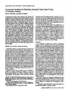
Figure 1.1: Motifs that have been found to be relevant in biological networks: (a) feedforward loop, (b) bifan, (c) single-input, and (d) multi-input [57].

multiple-output systems). Figure 1.1 illustrates some basic biological motifs as found in [57]. This figure is important since it suggests that counting triangles and other patterns in a family of motifs is a means of characterizing and reflecting differences between networks, motifs bear resemblance to the definitions of parameters used in exponential random graph models, highlights the importance of specific neighbors and interrelations, and parallels electrical circuits and control systems.

Schwöbbermeyer [57] offers a concise presentation of

biological motifs. He states that motifs typically apply to directed/undirected/mixed, connected, simple, and loop-free graphs. The concept of motif frequency has been introduced as a means to compare large graphs. See also [62]. The frequency of a motif is the number of different matches of this motif in the overall network. As such, they align more with computer science-centric graph matching methods rather than a comparison of nonoverlapping cellular automata/machinery. Motifs were originally defined using patterns that occurred at a significantly higher rate relative to randomized networks; a reliance on a random (or other suitable) null model is deemed critical in the derivation and comparison of motif frequencies.

Phillip D. Yates


26

Another difficulty of the frequency concept is that multiple interpretations are possible. At a minimum, one has to determine whether or not edges and nodes can be shared when counting across a family of connected motifs. Once a definition is assumed, a Z-score can be computed using a probability estimate of the motif frequency in the observed network relative to that of a randomized network. For a family of motifs these Z-scores can be combined into a significance profile using a normalized vector of Z-scores. To simplify the size of the pattern space examined (Alon [66] catalogs the 13 unique 3-node patterns for bidirectional graphs, illustrates the 199 4-node directed patterns, and warns of over 9,000 five-node directed patterns), graphlets have been introduced to simplify the comparisons. Graphlets are small subgraphs that are typically limited to three to five nodes. Schwöbbermeyer provides a comparison of the motif significance profiles between the gene regulatory networks of E. coli and S. cerevisiae. A significance profile comparison can accommodate graphs with an unequal number of nodes and edges; but, its utility for comparing ‘small’graphs is questionable. Once a level of comfort with simple motifs has been established, Schwöbbermeyer claims that the great majority of motifs overlap and are embedded in larger structures. Apart from further damaging the credibility of a random network null model, this statement implies that a network comparison should compare both small blocks and larger (perhaps functionally motivated) clusters. He also cites several studies related to the use of motifs for network comparisons. In one, the authors found that a geometric random graph was a more suitable generating model relative to a scale-free random model in modeling the graphlet frequencies of the S. cerevisiae and D. melanogaster protein interaction networks. In another study based on an empirical motif profile for the D. melanogaster protein interaction network, he chronicles the use of motif frequencies as a classifier for discriminating various artificial network generating models. Based on the presence of various real-world pressures in network formation, Schwöbbermeyer makes the troublesome comment, “A single network generation mechanism may not be sufficient to resemble the structure of these networks.”Finally, he briefly discusses the convergent evolution of motifs in gene-regulatory networks and the evolutionary conservation of motifs in a protein interaction network.

Phillip D. Yates


27

Alon [66], one of the original proponents of motifs in biological networks, authored a text on a biological circuit approach towards systems biology. His definition of a motif involves a statistical determination of a feature/pattern relative to an ensemble of random networks; this approach has been linked with evolutionary selective pressures. In contrast to the qualitative treatment by Schwöbbermeyer [57], Alon’s approach has a more distinct mathematical emphasis on cellular control systems. Unlike a pure graph theorist’s simplification of an edge in a graph, Alon posits that repression or activation functions can assign a sign to an edge; weights can be combined to an edge via a model such as a Hill function or a MichaelisMenten equation. Comparable to a computer scientist’s view of an -omic network as a computational dynamic system, his elemental treatment of positive/negative autoregulatory systems (a.k.a., a motif), coherent and incoherent feed-forward loops, etc., is of established value in the understanding of biological networks. In a descriptive measure sense, Saramäki et al. [36] outline two descriptive statistics for motifs on weighted graphs - an intensity statistic that is the geometric mean of the edge weights, and a coherence measure that is a ratio of the geometric and arithmetic weight means. These measures were applied to, in part, directed metabolic networks. Such statistics are relevant since weighted motifs are viewed as an extension to the set of topologically equivalent subgraphs of a network. Regarding the biological interpretations of motifs, Rodr´ıguez-Caso et al. [22] suggest that an explanation for the overabundance of certain motifs in real graphs relative to random graphs is still under debate. Some have suggested that motifs relate with functional traits whereas others claim that motifs are tied to the rules of duplication and divergence governing genome evolution. Part of the theoretical appeal of motifs is that one can use them to decompose (or partition) a graph into a family of isomorphic sub-graphs. This can be attractive in the analysis of very large unlabeled networks where computational concerns abound. In our opinion, the more compelling case to be made for motifs is in their role as basic reactions or machines (or control mechanisms) in cellular processes. In contrast to social network analysts, counting various motifs for unlabeled nodes in a network may only hold interest for a biologist if it allows

Phillip D. Yates


28

him/her to characterize the complexity of the machine. We have the distinct impression that motifs, despite their varying definitions, are conceptual tools firmly ensconced in the systems biology landscape. Despite an inherent topological presence in a graph and their assumed or assigned functional interpretations, their use or involvement in network comparisons is complicated. If we do not assume that the nodes are labeled then we are confronted with a complex matching/counting problem. Adding either directions, to suggest energy transfer or sequential process order, or weights, to capture activation or repression factors, to the edges must be addressable. If we add labels to the nodes then the generality of a motif could be secondary to the specific function of the particular subgraph defined by the nodes. The ambiguous definition of a motif also creates complexity. Do we decompose a graph into motifs using a library of known patterns (nonisomorphic subgraphs or sub-cellular machines), determine a family of patterns/combinatorial combinations using the graph itself, allow or restrict the reuse of nodes/edges in the graph decomposition/motif counting exercise, allow the motifs/patterns to intersect versus forming a unique partition of a graph, account for interacting or dynamic motifs, accommodate graphs with a small number of nodes, etc.? Given this range of questions it seems apparent that a minimal consideration of motifs in any network comparison is necessary; but, to suggest their overuse could produce biologically meaningless, ambiguous, contradictory, and computationally burdensome results. A careful study of biological motifs could form the basis for another dissertation.

1.3.2

Protein Interaction Networks

Protein interaction networks are fundamental to the study of (systems) biology. Proteins acts as catalysts, transmit signals, transport and store molecules, and are generally involved in controlling and mediating the vast majority of biological processes in a living cell. Apart from being involved in the structural assembly of a cell’s components, proteins are involved in transcription, splicing, translation, and the organization of enzymes. See Börnke [59] for a short overview of protein interaction networks. Proteins are three-dimensional structures

Phillip D. Yates


29

comprised of amino acids; this structure determines a protein’s function. Proteins almost always fulfill their complex role entirely through interactions with other molecules such as low molecular weight compounds, lipids, nucleic acids, or other proteins. These interactions can involve associations with partner proteins or necessitate the formation of large protein complexes. Protein interactions can be both static and transient. (Protein-)protein interaction networks, commonly abbreviated as (P)PI networks, are a useful platform for developing a network inferential strategy. Protein networks are usually assumed to consist solely of nodes and edges; directionality is more readily applicable to gene networks. A tremendous amount of protein information is available in online databases. Chen et al. [14] provide a list of 16 databases that provide experimental (e.g., high-throughput) PI data; 8 databases devoted to ‘known’domain-domain interactions is also cited. Large PPI networks have been characterized as small-world scale-free networks, see references in [13]. Not surprisingly, Chen et al. [14] cite recent literature that call into question these descriptive forms. Various experimental techniques have been developed to study protein systems. One- and two-dimensional gel electrophoresis, affinity chromatography, yeast two-hybrid screening (Y2H), gene coexpression, synthetic lethality, protein arrays, and mass spectroscopy are some of the platforms used to study pairwise protein interactions [12]. Unfortunately, different methods can yield different and even contradictory results. Both Helms [12] and Zhang [13] state that the error rate of Y2H experiments is on the order of fifty percent. Many concede that high-throughput experiments are known to have non-negligible false negative and false positive rates [13, 12, 59]. Y2H, mass spectrometry, and protein arrays are among the most commonplace tools for investigating PPI networks. The sheer number of possible interactions one can survey presents a challenge. For yeast, Saccharomyces cerevisiae, there are approximately six thousand known proteins and roughly eighteen million possible interactions. Experiments routinely assay hundreds-to-thousands of proteins and suggest a comparable number of interactions. Helms [12] states that one

Phillip D. Yates


30

hundred thousand is a plausible upper bound for the number of interactions. Apart from the reliability of PPI data, Zhang [13] documents two other concerns in the computational analysis of PPI networks. A protein can have multiple functions and participate in various functional groups. And, two proteins with different functions frequently interact together; such interactions can complicate the topological complexity (and assumptions for a probability model) of PPI networks. She describes in detail some of the generic computational strategies used to predict protein interactions/function. Broadly, these approaches include: genome-scale (e.g., interspecies comparisons, gene fusion, phylogenetic profiles), sequence-based, structure-based (docking, three-dimensional architecture, interface properties), learning-based (machine learning tools, it is possible here to incorporate a range of biological covariates), network topology-based (topological analysis, distance-based modularity, graph-theoretic modularity), and integrating domain knowledge from an ontology tool such as GO.

1.3.3

Gene Networks

Unlike protein interaction networks, gene networks exhibit more variety in their form and function. Proteins are the workhorses in cellular functioning. The role of genes, while no less crucial, is more complicated due to their role as the initial substrate in the creation of proteins. At a minimum, transcription factors (a binding factor that inhibits or promotes transcription), post-transcriptional processing, DNA chromatin and epigenetic modifications, and translation steps are involved in the control and conversion of gene products into a functional protein. Potapov [58] is a brief synopsis of signal transduction and gene regulatory networks. Regulatory networks, which can consist of genes, proteins, and other biocomplexes, govern the rate at which genes are expressed in time, space, and magnitude. Since only a small portion of the genome is translated into proteins, determining the regulatory role of unexpressed DNA is an interesting problem relative to the evolution and existence of organisms. Potapov

Phillip D. Yates


31

claims that new phenotypes are more likely the result of new relations between existing genes/proteins rather than the introduction of novel bioagents. Regulatory networks, given their focus on the interrelationships between genes and their products in the cell, can subsume portions of protein, gene interaction, signal transduction, metabolic, etc., networks. Transcription factor networks, which capture the binding domains that actively promote or repress the transcribing of genes into mRNA, are a simpler example of a gene network. Relative to metabolic and PPI networks in select organisms, our understanding of regulatory networks is less comprehensive. Potapov [58] documents several of the online databases that serve as repositories for portions of these data. The topology of regulatory networks can serve as a structural foundation for representing these cellular systems; superimposing quantitative information is made possible by additional modeling and simulation. Similar to PPI networks, in select analyses these networks have been labeled as scale-free and small-world [58]. These networks can be weighted, (partially) directed, in some abstractions bipartite, and exhibit more complex properties such as anisotropy or auto-regulation. In signal transduction networks one can have nodes respond to stimuli such as steroid hormones, stress, and UV radiation. Transcription factor-gene networks may possess a hierarchical modular structure in bacteria, yeast, and mammals [58]. In the analysis of differential regulation in gene sets, where the gene set may be defined per regulatory function or documented in a domain database, the network structure may be ambiguous defined. Helms [12] states that ‘guilt by association’methods are popular for inferring gene networks; a view also applied to PPIs [13]. Genes with similar expression patterns are assumed to be functionally related. This assumption is amenable to both cluster and principal components analyses. Helms goes on to claim that these techniques may only work when the networks are modular and contain a small number of interactions; their use on heavily connected graphs may provide ambiguous results. The apparent complexity and diversity of gene networks will not be fully addressed in this dissertation. Rather, these networks serve as a reminder

Phillip D. Yates


32

of the (potential) complexities that an inferential strategy must consider in the construction of a viable comparative procedure.

1.4

Modeling Biological Networks

Modeling biological networks is a nontrivial process. Stolovitzky et al. [15], in the preface to their edited collection, state that the painstaking advances made in reverse engineering the p53, NF-κB, and β-catenin signaling networks, the E. coli transcriptional regulatory network, and the many known metabolic routes are the result of a, “Truly heroic and mostly experimental tour de force.”Given the possibility of complex spatio-temporal dynamics on a set of interconnecting processes, the assumption of a straightforward likelihood-based model stretches the imagination with regards to plausibility. In addition to level changes during the cell cycle, cellular processes have to respond to external stimuli. Reflecting the rate of these changes in a graph is challenging; some of this information may be able to be coded in a graph via a weighting scheme. Jeong et al. [65], in the introduction to their paper on predicting putative RNA-interacting residues in proteins, recount some of the approaches taken in the study of such a complex problem. These include analyses of specific RNA recognition modes in proteins, the binding properties of the protein-RNA interface, the chemistry of both specific and non-sequence specific binding, both atomic and molecular properties with secondary structural effect in hydrogen bonding, and the energetic features in protein-RNA recognition. They considered RNA-protein interactions formed by hydrogen bonding, stacking, electrostatic, hydrophobic, and van der Waals forces. Protein residue networks (or their variants) are not a specific focus here; we merely wish to reinforce that the complexity of interaction mechanisms seems ever present from atomic-to-macromolecular scales and both inside and outside the cell’s nucleus. Defining an edge in a PPI graph can be a function of physiochemical interface properties, sequence evolution and homolog behavior, energetic considerations, etc.

Phillip D. Yates

1.4.1


33

Of Mathematics and Machines

Viewing biology as an (electro)mechanical (or electrochemical) process is not new. Blossey [70] offers a discussion of computational biology from a statistical mechanics perspective. Ross et al. [16] highlight the use of macroscopic chemical kinetics in the construction of both a Turing machine (a universal computer) and a parallel computer via a bistable reaction system. Despite the conceptual excitement this may hold for chemical engineers and computer scientists, using control systems as a basis for cellular systems also offers advantages for biologists. For example, oscillations are known to play a role in the transcriptional control of genetic networks [16]. Helms [12], in his introductory text, offers basic insights into the use of ordinary and partial differential equations for modeling kinetic processes. He states that differential equations are a starting point for the quantitative modeling of gene regulatory networks. Their use allows one to study: the magnitudes of signal output/duration as a function of the kinetic properties of the pathway components, the coupling between signal amplification and speed, designs to insure that pathways are safely ‘off’in the absence of stimulation and ‘on’following receptor activation, how different antagonists can stimulate a sustained/transient response in the same pathway with dramatically different consequences. He provides examples of their use in modeling protein synthesis/degradation rates and protein (de)phosphorylation mechanisms. In comparison with components in a nonlinear control system, he cites their use in modeling toggle switches (mutual inhibition), one-way switches (positive feedback), buzzers, sniffers, and negative feedback systems (oscillators and homeostasis). These theoretical biology tools have yielded insights into the cell cycle and small molecular systems, e.g., bacterial photosynthesis. Not surprisingly, such approaches are more difficult to apply to the specification and study of large networks. Such models, apart from their use as biological machines, may be able to be incorporated into weighted graphs. Blossey et al. [64], after citing some of the limitations imposed by modeling biological networks via differential equations, suggest a computer science approach (machine) toward

Phillip D. Yates


34

modeling gene networks. Process calculi have recently been introduced as a programming language environment for concurrent and interactive systems such as mobile communication networks. These abstract systems are comprised of functional modules with simple rules governing self-behavior (e.g., rate of duplication or decay for biomolecular matter) and their interaction with other modules. Blossey et al. demonstrate the use of a π-calculus for simulating an artificial repressilator and several combinatorial gene circuits. Modules represent biochemical components; functions are defined to mimic cellular processes. They suggest the use of this calculus in hypothesis testing but acknowledge the difficulty imposed by the need to compare system output. Parameter sensitivity concerns, both in terms of quantitative strengths or qualitative relationships, are duly noted. However, a mechanism for performing hypothesis testing was not explicitly suggested. Cardelli [63], in a more expansive and thought-provoking paper prior to [64], suggests that we view cells as machines in the service of materials, energy, and information processing. He postulates the existence of three abstract machines: the protein machine (biochemical networks whose fundamental flavor is fast synchronous binary interactions), the gene machine (regulatory networks whose fundamental flavor is slow asynchronous stochastic broadcast), and the membrane machine (transport networks whose fundamental flavor is fluid-in-fluid architecture, membranes with embedded active elements, and fusion and fission of compartments preserving bitonality). He is forthright in recognizing the associated difficulties. Viewing a gene machine as a continuous or discrete process, both in time and concentration levels, is a major question. He suggests that qualitative models, e.g., random and probabilistic Boolean networks, asynchronous automata, and network motifs, can provide more insight than quantitative models, models whose parameters are hard to come by and of questionable criticality. After stating that all formal notations known to computing have been used to represent aspects of biological systems, he makes a resounding endorsement of the recent advances made in applying process calculi to biological systems. The Ambient (which extends the π-calculus to include compartments and complexes) and Brane (which embeds the two-dimensional operations and biological invariants of membrane networks) Calculi are

Phillip D. Yates


35

two platforms that suggest promise in this area. Whether or not these calculi could advance the likelihood tradition with non-identical functional building blocks is an intriguing idea.

1.4.2

Correlation Networks

It is conceivable to consider correlation, coexpression, or coregulation networks as a distinct form of biological network. Our emphasis here is on the use of a numerical (or other model-driven) form to model these network systems; this approach also makes the case for a weighted network self-evident. Unlike strict distributional forms, e.g., the multivariate normal distribution, correlation(s) can be defined in a broader manner. Caldarelli et al. [5] provide some simple examples of how correlations can be coupled to a network’s topology. One example, based on the current hub-model for airport traffic, suggested that associations can form on the basis of a current topology. I.e., correlations, apart from a higher moment effect, can affect a network’s architecture. Correlation networks tend to be highly clustered; investigations into the (dis)assortative properties of correlation networks may be inappropriate [56]. Steinhauser et al. [60] offer a solid introduction to -omic correlation networks. These networks, which are generally undirected due to an inability to derive a flow, sequence order, or functional role on the basis of a correlation, do not establish causality. They also lack an ability to separate primary and secondary effects, especially if these effects are timeordered. From a statistician’s perspective, the authors’ material is elementary. But, they argue (and demonstrate with several biological examples) that ‘correlation’models provide a more comprehensive understanding of cellular systems relative to qualitative (edge/no edge) or cell inventory (each individual node) quantitative models. As multiplex array and highthroughput sequencing technologies mature these networks could become more prevalent. The authors repeatedly stress the importance of data, experimental purpose and design, data collection, data quality, data processing, data analysis, and interpretation in making best use of these networks. Microarray normalization techniques, the impact of small sam-

Phillip D. Yates


36

ples on parameter identifiability, the variance introduced through imprecise measurement systems, etc., are brought out of the shadows. The classical Pearson product-moment correlation coefficient is not the only correlation measure employed. The use of robust measures such as Spearman’s ρ, Kendall’s τ , mutual information, and partial correlations are also used to form these networks. The use of partial correlations, intended to mitigate some of the effects observed with pairwise correlations, is discussed later in this dissertation. Testing individual correlations is (almost) inherent to forming correlation networks. Tests, especially in the case of a Pearson product-moment correlation or a Fisher’s z-transformation, for individual correlations are well documented in the classical literature. Translating a correlation matrix into a network requires a filter to convert real-valued numbers into (weighted) edges. This is generally accomplished via p-value thresholds, comparing the absolute magnitude of the correlation coefficient to a fixed value, or a combination of these two comparisons. The discretization process, either through the threshold choice or p-value influences such as sample size, is a known source of network misspecification. Steinhauser et al. [60] state that, due to the dependency of the estimated network on the correlation matrix, the “Analysis of correlation networks is just in its infancy.”In analyzing these networks one typically utilizes one of two methods. The first approach considers the entire network topology. In the second approach one chooses one or more ‘guide genes’from which to originate the analysis. The authors endorse selecting guide genes on the basis of biological knowledge, such as components of a signaling or biosynthetic pathway, components of a protein complex, or known subcellular localization or regulatory factors. They state that this kind of analysis is “Very similar to other function prediction machine learning techniques such as k-nearest neighbors or correlation based clustering.”

1.4.3

Inferring Network Structure or Topology

Inferring network topology for biological networks has been extensively studied. The complexity is considerable when one considers the array of biological mechanisms under study,

Phillip D. Yates


37

the number of organisms studied, and the number of algorithms available for (mis)use. Gutenkunst et al. [29] assert that complex biological models appear to be universally sloppy, i.e., the observed variation can be quite sensitive to different parameter combinations (a trait also exhibited in nonlinear multiparameter models) and that biologists place more emphasis on structure relative to parameter estimates. Unlike traditional parameter-centric testing procedures, this interest may induce one to separate edge (structural) distinctions from weight (parameter) distinctions. For another example, Ross et al. [16] indirectly cite, in their 2006 text, over 125 references devoted to the study of the molecular mechanism of cell cycle control in Saccharomyces cerevisiae. The resulting model for budding yeast has nearly 20 variables with that many kinetic equations and approximately 50 parameters (rate coefficients, binding constants, thresholds, relative efficiencies). They go on to state that a fair number of assumptions are necessary to accommodate the absence of substantiating experimental evidence and the need for approximations to simplify the kinetic equations. The text, with a noticeable slant toward the chemical kinetics of metabolic networks, goes on to detail a method based on pulse perturbations, offers a theory for the statistical construction of reaction mechanisms (a variety of statistical algorithms are applied to time course experiments), and the use of genetic algorithms for the determination of complex reaction mechanisms. At the risk of sounding droll, algorithms abound in the literature.

Computational and Statistical Learning When trying to survey the computational, machine or statistical learning, or other computerintensive approaches to modeling biological networks, one quickly realizes the impossibility of the task. Equation-wielding theoreticians pen articles that fill methodology journals; experimentalists embed a variety of models and methods in their ‘bench-centric’publications; and computational experts (e.g., bioinformaticians) fill in any intervening gaps. Incorporating data from multiple domains (gene/protein/metabolite, physiochemical covariates, or various databases) further complicates the computational landscape. The intent here is to

Phillip D. Yates


38

provide a judicious sample of the existing literature. Chen et al. [14] display a variety of techniques in their text on biomolecular networks. While distinctly emphasizing differential equations for gene networks, probabilistic models for protein networks, and optimization methods (i.e., integer and (non)linear programming algorithms) throughout, they also present graph-theoretical, combinatorial optimization, and matrix factorization/decomposition methods. They recount the use of association probabilistic and maximum likelihood estimation methods in inferring binary protein interactions. Unfortunately, convenient probability assumptions, e.g., domain-domain interactions are independent or conditioning the ability to interact on another interaction, can limit the predictive accuracy of these methods. [14] cites a study that was able to improve the statistical accuracy of protein function prediction by incorporating information beyond the adjacent neighbor(s) in the network. Wei et al. [178] use a local discrete Markov random field approach for identifying genes/networks related to a phenotype. Extending beyond the immediate neighbor(s) will be explored in this dissertation. Zhang [13], in a chapter devoted to statistical/machine learning methods, highlights the integration of Markov random fields and domain-based belief propagation databases, kernelbased methods (e.g., support vector machines), and a common-neighbor-based Bayesian method for protein function prediction. Jeong et al. [65] use a weighted-profile neural network approach to infer RNA-residue interactions in proteins. Husmeier [68] models gene regulatory networks using a Bayesian network approach; the expectation is to form a model that is an intermediary to small-scale coupled differential equation (bio)chemistry models and computationally inexpensive large-scale clustering models. In the same context, Rangel et al. [69] employ state-space models (linear dynamical systems). Saul et al. [179] explore the use of ERGMs in modeling biological network structure. As expected, some will question the utility of certain approaches. For example, Ross et al. [16], in their review of Bayesian networks for determining complex kinetic reactions, state that, “There is no rational basis, as yet, for connecting a Bayesian network with a chemical, biological, or genetic reaction mechanism: the equivalents of the concepts of temporal dynamics of reaction mechanisms,

Phillip D. Yates


39

of rate coefficients, and of reversibility of elementary reactions are missing from Bayesian networks.” Emmert-Streib et al. [11], in an edited collection of 14 chapters devoted to the analysis of microarray data from a network-based approach, contains a formidable display of methods and algorithms. Methods (or method extensions) include: Gaussian graphical models, (dynamical) Bayesian networks, probabilistic Boolean networks, an application of threshold gradient descent regularization, a LASSO-based EM algorithm, genetic algorithms, structural equations, generalized least squares, a generalized T 2 test statistic, a group SCAD penalization procedure, B-splines, random forests, entropy maximization methods, a delayed stochastic simulation algorithm, a recursive v-structure location algorithm, an average-cost-per-stage approach, etc. Such a proliferation of tools presents a challenge for molecular biologists (some of whom may readily admit their computational inexperience). Which of these methods are useful? For in silico, in vitro, or in vivo experiments? Does a particular model routinely underfit or overfit networks? If so, does this shed light on meaningful biological phenomena or destine the method to published obscurity?

Discovery via Discoverers As mentioned earlier, Raychaudhuri [18], and the extensive references therein, emphasizes the need and use for text mining techniques in genomics research. In addition to the challenge of tracking the (voluminous) scientific literature for a single gene, the author makes the compelling case that mining the available literature is necessary to put experimental data into a meaningful biological context, a shortcoming of purely numerical approaches for analyzing these data. He explores methods to mine the literature to propose gene networks and to confirm protein interactions suggested by experimental data. The extent to which such tools actually shape the ontology databases, e.g., Gene Ontology and KEGG, is unknown to this author. The measures used to compare documents are broadly related to sequence alignment procedures and other similarity measures.

Phillip D. Yates


40

Raychaudhury [18] mentions the gene annotation process in GO and emphasizes the importance of the “traceable author statement.”Other high quality annotations are obtained from direct experimental data. Much less reliable are “inferred from sequence similarity”or “inferred from reviewed computational analysis.”Even less reliable are the “inferred from electronic annotation”annotations that have been transferred from electronic databases or other electronic searches and have not been reviewed by any curator. He goes on to state that KEGG deals with gene functions from over 100 organisms and seeks to provide a unified resource for structured information about genes, protein-protein interactions networks, molecular pathways, and chemical intermediates. The PATHWAYS database, in part, contains manually compiled networks of functional significance. Text mining tools offer yet an additional source of variation in determining nodes and edges in inferring network structure.

1.4.4

Validating Models

Surveying the panoply of methods used to validate network models is a daunting task. For every published algorithm or modeling approach that seeks to infer a protein interaction or suggest a novel transcription factor-gene interaction, some form of validation is possible. A validation approach suggests that a comparison of two networks takes place. The amount of rigor and vigor used in this process can vary; some acknowledge the difficulty of the problem [68, 69]. Kahlem et al. [27] detail three approaches to the ‘experimental validation’of a model. One method would introduce a perturbation that is experimentally testable, another challenges the model with a previously unused set of measurements (e.g., training/validation data sets), and the third approaches relies on reconstructing a correct system using in silico or in vitro synthetic system data. The DREAM initiative, which held its 4-th conference in late 2009, is dedicated to the Dialogue for Reverse Engineering Assessment and Methods [15] and openly tackles the question of validating network models. Husmeier [68] even suggests that some modeling/validation efforts, although well-intentioned, can lead to erroneous conclusions. While it is understood that false positive rates for inferring interactions can be

Phillip D. Yates


41

high, Reddy et al. [82] cite false positive rates in excess of 50% for widely used algorithms predicting transcription factor binding sites. Pinpointing the source of the error can prove difficult. Husmeier made reference to false positives that are indirectly the result of sequence information and not of an actual biological interaction. Huang et al. [83] cite false positive rates of 25 to 45% for yeast, worm, and fly protein interaction data. They also cite overall false-negative rates in the range of 75 to 90%; roughly half of the rate is attributable to statistical undersampling and 55 to 85% of the false-negative rate is due to proteins that were systematically lost from the assays. For purely deterministic models, such as differential equations, comparing experimentally obtained time course expression profiles with simulation data is common [66]. Some comparisons may not even be formally validated or tested, especially for relative comparisons. [71, 72, 57] merely graph topological properties across multiple species. If a network’s degree distribution can be approximated by a power-law function, one might argue biological parallels from that simple observation (especially if a clustering coefficient supports a smallworld model). Perkins [28], in his differential equation study of the gap gene developmental network for Drosophila melanogaster, found the use of data-driven model validation procedures problematic. His efforts at using cross-validation and other resampling schemes found that the training and test errors were highly correlated. He attributed this, in part, to the correlations induced by the use of an array platform and how the data was processed (e.g., image alignment, background subtraction, and spatial averaging). Computational analysts/biologists can evaluate a method’s efficacy with both simulated and real biological data. In the first case an inferred network based on a fixed model is compared to the known network; in the second (and closely related) case one can compare estimated relationships/interactions with a ‘gold standard’extracted from a reputable online database. Chen et al. [14] provide two examples, each using a different algorithm, in the analysis of E. coli and Arabidopsis thaliana gene regulatory networks. Since biological meaning resides in the details, gene lists that document correct hits/misses and potential novel interactions often accompany these analyses. These lists can provide a source of much discussion and

Phillip D. Yates


42

(dis)comfort for biologists. Comparisons to a known network naturally gives rise to true positive, false positive, etc., sensitivity, and specificity concerns. Similar to microarray studies, nonoverlapping/intersection comparisons implicitly involve the benefit of the proposed discoveries. False positives may be more tolerable in the presence of an overwhelming true positive rate. If the algorithm incorporates an ordered quantity, e.g., a threshold or tuning parameter, one can generate receiver operator characteristic (ROC) curves. Husmeier [68] used receiver operator characteristic (ROC) curves to gauge the extent of spurious gene interactions via a pure simulation approach for a Bayesian network algorithm. In addition to the use of ROC curves, [65] gives other measures of prediction performance (e.g., total accuracy, accuracy, sensitivity, specificity, and Matthews correlation coefficient) in their neural network approach to inferring RNA-residue interactions in proteins. These measures appear to be common in Boolean network comparisons. Probabilistic networks, where binary interactions can be modeled across an ensemble of random networks, can give rise to observed difference-divided-by-expected summary measures [14]. At the initial DREAM conference, ROC and precision-recall (PRC) curves, where precision is related to false positives and recall is related to false negatives, appear to have been the method-of-choice for validating network models [26]. In addition to comparing to a known ‘gold standard’, Stolovitzky et al. [26] advocate the use of blinding. If and when possible, blinding the computational investigator to the actual network can prove especially useful in in silico reverse engineering efforts. In validating models a score function is often employed. Chen et al. [14], in a section on the use of singular value decompositions for reconstructing gene regulatory networks, suggested E0 =

n ∑ n ∑

I∥JijT − JijR ∥ > δ

i=1 j=1

to compare an estimated network with a known network. I is 1 if ∥JijT − JijR ∥ > δ and 0 otherwise. δ is a small error tolerance related to the noise level of the system. JijT and JijR are the interaction strengths from gene j to gene i in the true and inferred networks,

Phillip D. Yates


43

respectively. Similar to E0 , they also suggested the use of both E1 = E2 =

n ∑ n ∑ i=1 j=1 n ∑ n ∑

I∥JijT − JijR ∥ , and I(JijT − JijR )2 ,

i=1 j=1

where E1 and E2 use the same notation as E0 . In suggesting an objective function for use in a mathematical programming approach, variants of E0 were used. For example, to help impose sparsity on the inferred network a tunable λ|Jij | term might be added to a weighted E0 ; another example minimized the total absolute error between predicted and experimental expression values. When multiple domains (e.g., protein interaction, protein complex, domain fusion) are combined to infer interactions, Chen et al. provided an example of an overall composite sore that was an arithmetic weighted combination of the individual scores, e.g., Stotal = ω1 S1 + ω2 S2 + ω3 S3 . Network validation can also suggest similarity between nodes and groups of nodes in the same graph. (This is comparable to block models in SNA.) For example, Steuer et al. [56], in their presentation of global properties, define a matching index for comparing two vertices in the same graph. Such intragraph measures resemble clustering coefficients or inter-cluster ‘significant’separation measures on a single graph; such approaches have been used in the modular analyses of PPI networks[13]. Cho et al. [183], in outlining a method to identify differential co-expression in gene sets, use a form of Renyi relative entropy to measure the similarity between gene expression matrices. The use of bootstrapping does not appear to be widespread in validating network models. We conjecture that this may, in part, be due to the distinction between methods that analyze raw data, e.g., microarray measurements, versus methods that manipulate graphs (obtained from an online repository). Fixed network comparisons also allow one to avoid the tedium (or intellectual audacity) of defining a probability model for the target network. Wiuf et al. [48] employ parametric bootstrapping in their full-likelihood approach to the analysis of network growth models. Zhang [13] suggested the use of a leave-one-out method to gener-

Phillip D. Yates


44

ate specificities and sensitivities in a Markov random field model for protein annotations. Rangel et al. [69], in their use of state space models, did suggest the use of bootstrapping to locate reliable gene-gene interactions; individual node effects were also examined via bootstrap confidence intervals. Li [23] is another example which makes use of bootstrapping, this time for a Gaussian graphical model approach. Toh et al. [170] use bootstrap samples to repeatedly produce estimates of a partial correlation network; the reliability of an edge was calculated using the percentage of times the edge was present across all of the network estimates. Emmert-Streib et al. [25] combine a permutation-based procedure with a graph-edit distance measure, a graph matching approach discussed in the next section, for comparing disease pathways. (Incidentally, this paper also assumed that the nodes were aligned and labeled. The pathways were not weighted.) Xiong [24], in a structural equation modeling approach for genetic networks, provides an algorithm for identifying differentially regulated networks. The method involves identifying model parameters for a network, uses a permutation procedure to test for the largest element-wise difference in a matrix of parameter estimates, and suggests the use of matrix differences and various matrix norms (e.g., L1 , L∞ , L2 , and Euclidean norms) in comparing networks. These topics bear a direct relation on the methods developed in this dissertation.

1.5

Comparing Networks

Unlike real-valued objects, e.g., a population mean, comparing nontransient networks is nontrivial. If we view a cellular network as an electrical machine, how can we compare two machines? (This is analogous to comparing an iPhone with an iPad - both are effectively computers with comparable components/functions but with vastly different intended uses. The comparison is made apparent by design.) Unlike classification or prediction tools, what is the appropriate residual variance or misclassification rate to minimize? Comparable to the iPhone/iPad comparison, is there a straightforward loss function that is independent of a priori context? For the biophysicist, how does he assess the quality of a deterministic or

Phillip D. Yates


45

stochastic differential equation? Resorting to simplicity, such as drawing a picture of the inferred graphs under comparison, does not offer a robust solution. It is broadly acknowledged that visual representations or pictures of graphs can be misleading. Helms [12] offers some basic guidelines for visualizing biomolecular networks: the graph should contain a minimal number of edge crossings, the graph should emphasize any symmetries that are present, and the vertices should be evenly spaced. Cook et al. [41] review three popular approaches for drawing graphs, namely, the force-directed, the hierarchical, and the topology-shape-metrics approach. Unless a visual comparison between two graphs is stark, these approaches do little to uniquely quantify the (probabilistic) differences between (large, complex) graphs. If one views each node in a graph as a subspace of a high-dimensional space, the assumption adopted here, then visualizing a graph in the plane is a clear misrepresentation of the data. This assumption will motivate our use of a set/neighborhood in defining network separation; it also limits the use of fractal/scale-invariance comparisons found in [6]. One of the challenges in comparing biological networks is the tremendous amount of context associated with, or superimposed on, a network. For example, [22], in their human transcription factor network study, define a self-interaction as an interaction between proteins of the same type, i.e., homo-oligomerization, regardless of the number of monomers involved in the interaction. They go on to observe that 17.8 percent of the proteins in this network have self-interactions and claim this to be a high level. A contrast of the correlation profiles for the network, both with and without the self-interactions, was tied to the biological constraints of the phylogeny of transcription factors. They state, “From a structural point of view, the over-abundance of self-interactions is associated with a majority group of 55% of basic helix-loop-helix (bHLH) and leucine zippers (bZip), a 17.5% of Zn fingers, and a 22.5% corresponding to a more heterogeneous group, the beta-scaffold factor with minor groove contact.”This quote suggests the ease with which biologists can impose structural/ functional similarities onto a network on the basis of observed clustering/a modular architecture. How best to integrate this type of information into a vertex/edge/weight abstraction can be unclear. Moreover, others could then be tempted to propose and use the structural

Phillip D. Yates


46

or relational properties of gene sequences or proteins to (fail to) differentiate networks under study.

1.5.1

Identifying H0

In order to compare networks one must give consideration to the mechanism or environment that results in a network’s formation. Unlike the traditional-yet-defensible “collection of independent and identically distributed normal random variables”assumption applicable to an astonishing array of scientific problems, network generating models is a compelling research topic in its own right. In contrast to the normal (Gaussian) distribution, whose theoretical origins appeal to empiricists but whose utility as an error distribution resides in its ability to reflect natural phenomena, man’s role in defining network models is apparent. Again, mathematicians, computer scientists, physicists, etc., offer unique perspectives on assigning form to nature’s behavior. Even producing a ‘random’graph, a mathematical abstraction with no duplicate links, isolated nodes, loops, or multiple components, can prove challenging. Lewis [4] captures two such approaches, one by Gilbert and another by Erd˝os-Rényi. One begins with a fully connected graph and then randomly removes links until the desired link density is obtained; the other inserts links between randomly chosen node pairs until the desired number of links is achieved. Since both methods can produce graphs with disconnected components, he provides an anchored generative algorithm that sacrifices a bit of randomness for a connected graph. The Barabási-Albert (BA) model dynamically grows a network contingent on an existing node’s degree distribution, i.e., via preferential attachment. The BA model has been extended to incorporate fitness measures, edge growth mechanisms, and aging effects (e.g., diminishing social ties), to name a few [6]. The Watts-Strogatz small-world model, a graph with a high level of local clustering and a short path length, is most often illustrated by rewiring together a few random nodes in a 2-regular circular graph, a graph where each node is connected to its four immediate neighbors, two on each side, on the circle. Transi-

Phillip D. Yates


47

tioning from a nonrandom regular graph to a ‘slightly’random small-world graph has been linked to the presence of phase transitions (e.g., Ising effect) and the ability for a network to synchronize [4]. ERGMs, under a fixed parameterization, can use various insertion/deletion schemes coupled with acceptance/rejection sampling techniques to generate a family of networks drawn from a given distribution. Generating networks that follow a predefined set of topological features, e.g., a specific degree or path length sequence, can be achieved in a similar computational manner. Caldarelli [6] cites network models that employ copying or duplication mechanisms (e.g., web page creation, evolutionary conserved sequences), fitness measures (e.g., beauty, available traffic capacity), or have a basis in optimization/economic procedures (e.g., the Kleiber relation between body mass and metabolic rate, cost functions, transport mechanisms). Correlation networks, as discussed earlier, are defined using a (non)parametric measure that is thresholded. This approach assumes an additional layer of ‘data processing’to produce a network. Brandes et al. [40] also contains a useful discussion of network models. The focus on network models here is central to the discussion of network comparisons. In fact, Steuer et al. [56] state that, “The most crucial and probably most widely underestimated aspect of complex network analysis is the statistical testing of network properties.”They claim that the most difficult aspect of complex network analysis is the choice of an appropriate null model or null hypothesis. In most applications, the numerical indices computed for a graph are (or should be) associated with biological meaning or interpretation. The ability of these indices to discriminate between compelling biological phenomena is critical to their utility. Steuer et al. [56], in their discussion of null generating models, recap the unfortunate selection of random graphs in performing this critical task. Emmert-Streib et al. [25] provide a specific example of this in their comparative analysis of disease pathways. In [25] an ensemble of random networks with the same number of nodes and the same mean number of edges served as the null model in their comparative analysis. Comparing a characterization of a scale-free small-world graph against an Erd˝os-Rényi random graph null model does not provide a meaningful test of a protein interaction network. One may as well reject the

Phillip D. Yates


48

null hypothesis in advance of any actual calculations. To circumvent such a comparison, one may assume that some trait of the network, e.g., the degree distribution, serves as a suitable comparative measure. Unfortunately, this is an arbitrary choice; extending the choice to include features such as motifs, path lengths, etc., to generate an ensemble of surrogate null networks that are useful abstractions of complex biological processes is far from straightforward. Steuer et al. detail how the construction of metabolic and correlation networks intrinsically differ from that of random networks.

1.5.2

Isomorphisms and Deformations

Computer scientists, as practitioners of applied graph theory, have a deep interest in comparing graphs. Comparing graphs on the basis of structural features has applications in pattern recognition and computer vision systems, CAD/CAM tools, and molecular matching problems, to name a few. Brandes et al. [40] and Cook et al. [41] offer an excellent survey of an area that has been under development for more than thirty years. Computer scientists typically divide the graph comparison problem into two areas - exact graph matching and graph similarity. In exact graph matching the interest is on establishing the structural equality between two graphs. Mathematicians term two structurally identical graphs, G1 and G2 , as isomorphic. Isomorphic graphs share the same number of vertices, edges, degree distributions, connected components, centrality indices, spectra, etc. To date, no one has been able to give sufficient conditions that would allow one to determine if two graphs are isomorphic in polynomial time, i.e., the complexity status of the problem is unknown [40]. In contrast, the subgraph isomorphism problem is known to be NP -complete. Given the highly restrictive (and of limited practical utility) definition for isomorphic graphs the notion of graph similarity, or graph matching, has been developed. The importance of graph similarity is its ability to deal with errors or distortions in the network data. Three broad strategies have been developed to tackle this problem: identify the maximal common subgraph between G1 and G2 , a comparison which uses a combined difference of path lengths based on all pairs

Phillip D. Yates


49

of vertices, and the notion of an edit distance. The edit distance, which bears resemblance to the measure outlined in this dissertation, was first developed for use in string matching. The idea is to use basic graphs operations, node/edge insertions/deletions/substitutions, to transform G1 into G2 . The number of edits required to complete the transformation is directly related to the similarity between two graphs. These operations could also involve edit costs, e.g., the researcher may wish to penalize node insertions more than edge deletions. The earlier discussion on the use of network motifs to compare graphs via significance profiles is directly related to the problem of graph matching. Bollobás et al. [93], in a decidedly more mathematical exposition, discuss strategies for comparing inexact (random) graphs. They also discuss motif-like partitions and edit distance; they stated that these approaches were suited to examining ‘local’properties. They also suggest the use of metrics based on cut operations. Cut operations partition a graph and can allude to ‘global’properties. But, they are quick to emphasize the difference between sparse and dense graphs. The distinction is important since one of the key tools in the analysis of dense general graphs is Szemerédi’s Lemma and the accompanying embedding or counting lemmas. They reference several recent advances that have established the equivalence, in a Cauchy sequence sense, of specific subgraph and cut metrics for dense random graphs. For sparse graphs, a characteristic commonly assumed for biological networks and for which there is no satisfactory counting lemma, they propose a colored neighborhood metric in an attempt to capture both local and global graph properties. Their discussion appeared to be confined to binary, and not weighted, graphs and did not involve anything more than L1 or Hausdorff distances. Although not rigorously pursued in this dissertation, these findings seem to suggest that a ‘local’metric is more easily motivated in (very) sparse graphs with little loss of information on dense graphs. In contrast to the view adopted in this dissertation, graph matching is typically limited to unlabeled graphs. Emphasizing the structural similarities of graphs presents a more interpretative and complex problem for computer scientists; but, to dismiss a gene’s or protein’s identity is questionable from a practical standpoint. Consider two stick-figure-persons drawn

Phillip D. Yates


50

by a child as networks. Erasing a head (node) in one figure and a hand in the other results in two graphs that match. The biological implications are far different. An inferential strategy for comparing labeled graphs is a more analytically tractable problem; but, the ability to align nodes in a labeled graph was not assumed to trivialize computational matters. Drug investigators are interested in the effect of a compound on (targeted portions of) a biological network; unintended effects are also of interest if exhibited in non-targeted portions of a larger network. If phenotypic differences between two genetic networks are observed, efforts will most likely immediately shift to isolating the specific aspects contributing to the observed differences and their biological relevance.

1.5.3

Topological Parameters

Comparing networks on the basis of pure topological considerations is difficult. Apart from knowing which topological features adequately describe or determine the architecture of a graph, one can not overlook scaling aspects. For example, mathematicians continue to study the existence and emergence of a giant component, a connected component whose number of vertices is proportional to the total number of vertices in a given graph, in both random and power-law graphs [92, 90, 91]. Giant components have an intuitive connection to clustering in a given graph. Even for Erd˝os-Rényi random graphs the (potential) presence of a giant component depends on a complex interaction between the probability parameter p and the number of vertices in the graph. This impacts the ability to partition a graph into a disjoint union of trees, the existence of various cycles or loops in a graph, and how ‘small’components interact with ‘large’components both in number and degree of connectivity [90]. It can be possible to induce a phase transition in a graph, i.e., cause a giant component to emerge, just by adding a few edges to a graph near a phase boundary. Extending these concerns to weighted (directed) graphs is almost certain to invite even more complexities. A measure of separation that is not intrinsically tied to, or scales independently of, the number of nodes has obvious merits.

Phillip D. Yates


51

Table 1.1: Power law exponents for biological and nonbiological networks [90]. Biological networks Yeast protein-protein net E. Coli metabolic net Yeast gene expression net Gene functional interaction Nonbiological networks Internet graph Phone call graph Collaboration graph Hollywood graph

exponent β 1.6, 1.7 1.7, 2.2 1.4 - 1.7 1.6

2.2 (indegree), 2.6 (outdegree) 2.1 - 2.3 2.4 2.3

Even a comparison of the degree distribution is subject to statistical considerations. Similar to traditional goodness-of-fit tests, overlaying distributional qq-plots is common. For example, Maslov et al. [72] separately plot both in-degree and out-degree distributions for the human, yeast, and E. coli transcription regulatory networks. A visual assessment of these plots suggested differences between the species only for the in-degree distributions. Stumpf et al. [61], in their examination of protein interaction and metabolic networks for five species (D. melanogaster, C. elegans, S. cerevisiae, H. pylori, and E. coli ), found that both the lognormal and stretched exponential distributions served as better statistical models for the degree distribution of these two networks relative to the other distributions fit. In addition to these two distributions, the Poisson, exponential, gamma, and three forms of scale-free distributions were fit to these same data and compared with log-likelihood scores, via an Akaike weighting scheme, and using Kolmogorov-Smirnoff and Anderson-Darling goodnessof-fit tests. While admitting the limitations of these data, these authors call into question the wide-spread preference for scale-free models. In order to calculate maximum likelihood estimates under the various models these authors assumed that the nodes in the graph were independent observations; this (convenient) assumption seems to belie the definition of a network. Table 1.1 compares the power law exponents for various networks [90].

Apart

from the variability in these estimates, does this information expand our scientific under-

Phillip D. Yates


52

standing of these complex systems in a meaningful manner? To conclude our examination of degree distribution comparisons we recap an interesting discussion of the potential origins of power-law functions found in Caldarelli [6]. Caldarelli demonstrates how power-laws can arise from diffusion limited aggregation (or other forms of Brownian motion), minimization principles linked to entropy, dynamical evolution (e.g., self-organized criticality), multiplicative processes (e.g., the heavy-tailed lognormal distribution), or from thresholded/sampled exponentials. Determining a generative model for network data from a versatile, and biologically plausible, set of competing mechanisms is troublesome. Topological comparisons can also disregard biology (or mask data-collection bias). Rodr´ıguezCaso et al. [22] provide a (potentially) useful illustration of this in their analysis of a 230node graph of the human transcription factor interaction network (HFTN) obtained from a database. Although acknowledging the limitations of the extracted network due to our current understanding of the HFTN, they go on to state that the topological properties of the HFTN are comparable to other observed protein networks. They found that the HFTN correlation profile, discussed in the section on motifs, was similar to the yeast proteome profile. In their specific discussion of the top 9 proteins with the largest number of interactions, apart from the obvious TATA binding protein, 6 of the 8 remaining proteins were related to cancer (i.e., tumor suppressor proteins or proto-oncogens). Does a (limited) comparability between the HFTN and yeast proteomes suggest the presence of similar cancers or dominating regulatory mechanisms in yeast?

1.5.4

Sequence Alignment

Sequence alignment is another immense area of research. At a minimum, the fact that DNA consists of four nucleobases (cytosine, guanine, adenine, and thymine) has made comparing genomic sequences an integral part of genetics and bioinformatics. Even pairwise sequence alignment for DNA, which is known to have regions of inserted/deleted genomic material (indels), single nucleotide polymorphisms (SNPs), and to a lesser extent copy number variants,

Phillip D. Yates


53

inversions, and translocations is a challenging problem. Computer scientists have naturally been drawn to the area as a source of rich, computationally complex problems. Gusfield [42] authored a book on string and sequence matching from a computer science perspective where the intended application was computational biology. For a computer scientist, the problem of aligning sequences is comparable to the (in)exact (sub)graph matching problems discussed in a previous section. Deonier et al. [102] contains two chapters devoted to the basics of sequence alignment in computational genomics. In spite of the breadth of the subject, our treatment of sequence alignment will be brief. As captured earlier, aligning protein sequences across species has been used to locate novel protein interactions by integrating known interactions with sequential homology information [13]. Homologs are two related sequences, e.g., genes or loci, whose similarity originates from a common ancestor. In a limited or restricted sense, comparing networks is analogous to comparing a sequence comprised of a finite alphabet (e.g., A, C, T, G). This comparison of shared characters is fundamental to biologists. Sequence aligners have to wrestle with sequence homology versus sequence similarity problems for both global and local alignments. Complex scoring models, to account for just indels and SNPs, on uneven lengths of genomic material have been developed. Bioinformaticians have amassed an impressive array of computational tools (PathBLAST, NetworkBLAST, MNAligner, etc.) to use for aligning biomolecular systems [14]. We also seek to determine a scoring model, with an emphasis on weighted (directed) topological/functional structures, for comparing/differentiating networks and to aid in identifying relevant substructures. However, we will assume at the outset that we are able to align the nodes.

1.5.5

Orders of Magnitude

In wishing to advance the analysis of networks one has to consider the network’s ‘size’. Motifs, best exemplified by the 3-node feed-forward loop, exist on a microscopic scale. As illustrated earlier, physicists have been drawn to modeling large-scale graphs. Their ap-

Phillip D. Yates


54

proach may be ideally suited for the Internet or massive communication networks. However, compelling biological problems exist at both ends of the node- or edge-dimension spectrum. A pharmacologist may be interested in the cascading effects of small-scale disregulated systems; evolutionary biologists may find excitement in inter-species proteomic comparisons. Rodr´ıguez-Caso et al. [22] offer their perspective on the use and limitations of large-scale cell biology network studies. Some of their comments are listed below. • Graph theory is an adequate approach for large-scale networks and provides a suitable framework for modeling these systems. • Analyzing a network’s topological features can be used to identify candidates with potential biological relevance. • The topological form of a network definition implies a loss of information due to the need for simplification. For example, how can one integrate sequential assembly processes into protein map definitions? • Our current understanding of different molecular networks is far from complete. Furthermore, distinct molecular networks are partly embedded inside large, layered networks comprised of metabolic, protein, and gene regulatory systems. An ability to compare ‘small’networks, where topological comparisons could be highly discretized or meaningless, is an analytical prerequisite for an effective inferential strategy.

1.5.6

Testing Covariance & Correlation Matrices

In a previous section we presented the use of correlation networks for modeling biological networks. As we shall duly note in the next chapter, matrices are commonly used to represent graphs. As such, the network inference approach adopted here bears resemblance to oneand two-sample tests for covariance and correlation matrices. This correspondence makes clear that ‘traditional’or more customary statistical procedures may also be available for

Phillip D. Yates


55

testing network hypotheses under select network probability models. The literature for these comparisons, under both large sample theory and resampling approaches for a variety of applications, is substantial. We’ve restricted our discussion here to the comparison of covariance and correlation structures since these are used later to motivate and determine biological networks. It is not our intent to provide a detailed comparison of our proposed method to a traditional procedure, should such a procedure exist for a given network model. Many large-sample results do not apply to -omic data due to the prevalence of n ≪ p data. For example, in a classical test of a p-dimensional covariance matrix, H0 : Σ = Σ0 , the sample size is assumed to be much larger than p and the distribution of the test statistic requires (p) + p degrees of freedom. The use of resampling procedures can allow for more freedom in 2 defining a suitable test statistic since we are not constrained by a need to derive an exact distribution for a particular test statistic. Our intent is to outline a method suitable for a range of network models rather than create an ‘optimal’procedure defined under a limited set of assumptions. Anderson [136] is a classical reference outlining large-sample tests for (partial) correlation coefficients, canonical correlations, and various tests for covariance matrices. In a similar pursuit, Puri et al. [137] contains a discussion of rank tests for the homogeneity of dispersion matrices with and without the specification of location parameters. Steiger [138], Steiger et al. [139], Krzanowski [140], Schott [141], and Shipley [142] focus on tests for correlation-related matrices. Investigations into the use of the bootstrap or other resampling procedures are common in more recent methods devoted to the analysis of covariance matrices [143, 144, 145, 146]. Anderson [147], in a more recent development, uses a distance-based dissimilarity measure, a multivariate extension of Levene’s test, for comparing dispersion matrices. To address issues common to biological and ecological data, e.g., more variables than observations, nonnormal and zero-inflated data, the approach advocates the use of permutation procedures for determining p-values. In an unrelated vein, Manly [95] illustrates the use of the Mantel test for testing the correlation between two matrices in a biological application. Butts et al. [54] present an algorithm and useful references regarding the graph

Phillip D. Yates


56

covariance between two adjacency matrices. Comparable to Manly, these matrices can be used in a hypothesis testing framework contingent upon row and/or column exchangeability assumptions.

1.6

Problem Statement

Network analysis presents an exciting new frontier for statisticians. Unlike the rich tradition afforded by likelihood theory, network models are required to encapsulate complex interrelationships, are subject to dynamic phenomena, can be generative in nature, are in part measure both theoretically immature and inadequate, and need to accommodate a rich topological/graph-theoretic diversity. Their size can range from a 3-node feedforward loop to a representation of the yeast proteome. Many focus on analyzing the properties of a single ‘determined’network. An impressive array of measures have been proposed to summarize various graph-theoretic, topological, topic-relevant, or relational properties of a single network. Means and variances, so useful for real-valued random variables, have little relevance for objects defined by, at times vague or imprecise, interrelationships. Sampling, even for a single network, is a subject of current research. (This is most applicable to social and epidemic networks.) Dealing with a family of sampled networks, where each originates from an identical underlying probabilistic model, invites a broad array of statistical questions, many of which still appear to be in their developmental infancy. Even a clear demarcation of which network components are subject to random variability may be unclear. For example, in the yeast proteome some edges may be supported by a vast amount of experimental evidence and only exhibit uncertainty in the strength of the relation; other portions of the same proteome may contain estimated edges determined via a machine-learning algorithm and a variable weight obtained from a text-mining tool.

Phillip D. Yates

1.6.1


57

One- and Two-Sample Tests

In this dissertation we develop a comparative measure to aide in performing the equivalent of one- and two-sample tests. The measure can apply to networks consisting entirely of nodes and edges, include the addition of weights, and can be extended to directional networks or to accommodate node attribute comparisons. Our measure can apply to the situation where we assume a parametric model (e.g., the covariance matrix for a multivariate normal), are confronted with a network model whose parameter estimates defy large-sample asymptotic closed-form distributions (e.g., construct a ‘correlation’network from a family of pairwise Spearman ρ’s for data drawn from a multivariate T-distribution), and the nonparametric two-sample case. In forming our measure we avoid an explicit declaration of a network ‘error’distribution or model. In order to define a testing procedure we resort to a resamplingbased approach. The use of resampling or bootstrap-like procedures (which rely on messy real data and not a network extracted from an online database) is not revolutionary here; but, perhaps acknowledging a need for its greater use should be more carefully noted. Our measure avoids a comparison of ‘global’graph properties or parameters in favor of a more ‘local’element-wise comparison approach. But, our approach does not prevent or limit its use on scale-free small-world networks. Our metric is a logical extension of existing measures used in sequence alignment and other nominal data comparisons. In order to define a comparison, we assume that the nodes are aligned. This important assumption allows us to avoid comparisons involving critical missing covariates; but, the measure is still subject to bias in data collection or experimentation. In addition to sidestepping the computational complexities of graph-matching problems, this assumption allows for a welldefined comparison tied to biological function rather than graph-theoretic or topological characterizations. Data-gathering tools, e.g., modern array and high-throughout platforms, and data-repositories easily support such an assumption. Unlike a social network where the sampled actor nodes may be relevant primarily in a relational sense, our biological nodes should be viewed as individual variates.

Phillip D. Yates


58

The one-sample problem is not without difficulties. In a statistical comparison of a network with a target network, i.e., H0 : η = η0 , the target η0 is assumed to be known. The target may have been determined from a mixture of accurate and inaccurate data, e.g., been extracted from or derived from an online database. In the one-sample context we assume that η0 has an underlying known probability or generative model. We will state η0 in terms of known parameters or provide an explicit generative model; but, we acknowledge that the parametric form will likely fail as a reasonable surrogate for actual complex networks. An explicit declaration for η0 is directly applicable to correlation networks. In contrast to customary discrete or continuous random variables, realizing random networks involves a generative or formulaic process. As such, we are left in the unfortunate situation that in order to form an observed network estimate, ηˆ, we need some form of algorithm. To demonstrate our method, we have had to select several (basic) algorithms as demonstration vehicles. In focusing our application on array platforms, we assume that the biological sampling unit for the network is the organism. Each sampled organism is an independent realization of a transcription or protein interaction network under investigation. Certain interactions or coexpression levels can vary from organism to organism. This assumption is in stark contrast to social or epidemic networks. Such specimen data are often used in the analysis of time course microarray data or to infer networks via an algorithm. We conduct one- and twosample tests with simulated and actual microarray data obtained from the literature.

1.6.2

Post Hoc Comparisons

In evaluating regression models, whole model significance tests are often followed by individual (or a subfamily of) effect tests. A single severely disrupted coregulatory process in a tumorigenic pathway may prove fatal to an organism; a similar effect may occur when a portion of a regulatory network is adversely affected. If a single edge/node pair is primarily responsible for such a disruption, how can we identify the nodes? If a collection of

Phillip D. Yates


59

nodes/edges have been disrupted, what is an acceptable approach to identifying this subset of nodes with some amount of statistical rigor? In the construction of our test statistic, the metric is intrinsically multivariate. This suggests that we explore the sampling distribution of our measure, both for the overall composite score and the individual components, and provide insight into various diagnostic tools should a network difference be noted. The metric assumes, either implicitly or explicitly, that the measure of separation at a node is correlated with the measure at other nodes. (This is a direct contrast to probability models such as Markov random graphs.) Finally, we explore the properties of our approach under a variety of settings. Choosing these settings requires a measure of subjectivity; networks vary in terms of size, complexity (weighted or unweighted graphs), generative/probability models, (interdependent) parameters associated with a particular network model, are subject to theoretical and/or practical interests, etc. We examine the utility of our approach for both null and non-null cases. A brief discussion of computational details, e.g., execution time, and software modifications for particular applications, is also discussed.

1.6.3

Potential Applications

The utility of such an inferential approach is obvious. Many (most) scientific comparisons are to a known or fixed (ontological) standard or model, i.e., a one-sample comparison, or a relative comparison, i.e., a two-sample comparison. A molecular biologist may wish to know whether or not an estimated signal transduction network has significantly changed between times t0 and t1 , where the t0 -th network is assumed to be known. She may also question whether or not a protein network behaves differently under two stressors. In both cases, these networks may contain edges/weights that are estimated from experimental data. Novel algorithms are introduced almost daily and exploit the broad range of scientific and mathematical tools available for analyzing these data. Examples might include a new pro-

Phillip D. Yates


60

cedure to normalize array data or an algorithm to infer a regulatory pathway. The approach outlined here can apply as a diagnostic measure for evaluating algorithms. Given a sample of experimental data subjected to two different algorithms, a Bayesian network versus a support vector machine solution, do the resulting algorithms produce different networks? If so, what is a reasonable indicator of where they differ? Does an algorithm tend to underfit or overfit? Do they suitably recover edges but perform poorly when inferring weights?

Chapter 2 Dissimilarity: One-Sample Comparisons Measures of separation for network- or graph-like objects have taken a variety of forms. Hubert et al. [104] and Gan et al. [101] have outlined the use of ultrametrics, using either a L1− or L2−norm, in hierarchical graph-like applications. Unlike hierarchical cluster analysis or applications of dendrograms to visualize structure among objects, our conceptualization of a biological network lacks an inherent hierarchy. If one considers an observed network as a realization of a stochastic process, the view adopted in this dissertation, then other measures have been proposed for measuring stochastic separation. Kesidis [132] offers some basic definitions of separation between two distributions; several examples are listed below. For cumulative distribution functions F1 and F2 the Kolmogorov-Smirnov distance is defined as d(F1 , F2 ) = max |F1 (x) − F2 (x)|. x∈R

The Fisher separation for two distributions with means µi and variances σi2 is |µ1 − µ2 | . σ12 + σ22

61

Phillip D. Yates

Chapter 2. Dissimilarity Measure

62

Given two probability mass functions p1 and p2 on the same state space one can define their chi-squared separation as

∑ (p1 (x) − p2 (x))2 p1 (x)

x

.

The entropy of a probability mass function p with strict range R is defined to be ∑

p(x) log p(x).

x∈R

This important definition gives rise to the Kullback-Liebler distance between the entropies of two distributions,

∑ x∈R

p1 (x) log

p1 (x) . p2 (x)

This list is not intended to be comprehensive; but, an explicit reliance on a probability model is apparent. Borgelt et al. [123] document a more extensive catalog of measures for use in graphical models. These concepts are cited here since they reveal some of the difficulties associated with measuring a separation between two random network observations. There are at least two challenges to overcome in forming a comparison of two random networks. The first difficulty is apparent when one attempts to derive a test for the one-sample case. The challenge stems from determining the distribution of a suitable test statistic under the null hypothesis. Standard bootstrapping techniques can circumvent such difficulties in common parametric models, e.g., H0 : µ = µ0 versus H1 : µ ̸= µ0 . Here, it is plausible to assume that the distribution of the test statistic, based on x¯ − µ0 in this case, is symmetric about 0 under H0 and that the sample observations are merely shifted away from µ0 when H0 is not true. Large sample theory may be available to provide limiting distributions. But, determining the null distribution of a test statistic for an undetermined network probability model is not possible. Forming one-sample tests is understood to be a difficult problem for complex hard-to-specify probability models; Zhu [96] is a recent monograph on the subject. The previous chapter documented how some choose to adopt an Erd˝os-Rényi random graph as a null model; but, despite its mathematical tractability its probability mechanism is too limited to model observed networks. This lack of an apparent probability

Phillip D. Yates


63

model will impact our ability to use resampling procedures. Second, unlike traditional probability distributions with familiar (and often parsimonious) location and scale parameters, specific parameterizations for network distributions are lacking or are motivated by specific applications. Examples of this were cited in the earlier section on social networks; parameters for an ERGM are often chosen to reflect the social phenomena under investigation. An ERGM parameterization is generally formed with count-based statistics on an unlabeled graph; the parameterization can also shape the allowed probability space in an unexpected or undesired manner. The difficulty of defining a parametric form for a (weighted) network probability function, much less a broadly endorsed probability form, is further compounded by the fact that closed-form distributions for analogous large-sample frequentist parametric tests have not emerged for network applications. The elegance of a Central Limit Theorem has not been derived for network applications. Section 1.2.1 highlighted the broad range of interpretation that a centrality measure can assume in social networks. (Defining a mean, median, and mode as a measure of centrality for a real-valued random variable is trivial, in comparison.) Entropy-based network comparisons have been developed using variants of the KullbackLeibler distance, a familiar concept for computer scientists and information theorists, where probability functions are induced from a single observed network and the target network. Lewis [4] and Ben-Naim et al. [34], using a discrete distribution on an integer-valued support, can define the entropy for a single graph. For example, [4] forms a discrete probability distribution based on the number of edges at each node. Theoretically, this ‘histogram’could be defined for a variety of count-based ERGMs; simple extensions to a joint distribution function are straightforward. Extending this basic form of entropy to a Kullback-Liebler distance is trivial in the presence of a second graph. Such measures, apart from the theoretical difficulties associated with entropy comparisons, can cause one to question whether or not the appropriate sampling distribution is employed. Such comparisons may be most appropriately viewed as a non-inferential descriptive statistic and reflective of intra-graph variability rather than inter-graph variability. Of course, in the presence of a probabilistic data generating

Phillip D. Yates


64

mechanism one could bootstrap a relevant sampling distribution; but, one would still be confronted with a need to select an empirical parameterization (degree, in- and out-degree, weight, clustering coefficient, path length, etc.) of unknown dimension in order to calculate the needed joint probabilities. In contrast to the simple examples of Kesidis [132], Webb [106] provides more sophisticated measures of separation for multivariate distributions. These include the Chernoff, Bhattacharyya, Divergence, and Patrick-Fischer measures. Webb states that these measures have limited practical utility due to their use of numerical integration procedures and the need to estimate the probability density function based on a sample. But, for multivariate normal distributions, with means µ1 and µ2 and covariances Σ1 and Σ2 , convenient closedform expressions exist for these measures. Since probability models for general networks are immature, a need for a method that can avoid explicit model definitions holds appeal. Apart from the number of nodes and edges intrinsic to any graph, additional graphical properties can be subject to range of context-dependent or data-acquisition concerns. Unlike real-valued random variables, given a collection of n independent and identically distributed stochastic graphs, {xi | i = 1, . . . , n}, a more subtle effect emerges when one considers that an intrinsic well-ordering of these xi graphs is not immediately apparent, we’ve lost our familiar Euclidean metric footing, and a network-parallel to statistical sufficiency has not been developed. Comparable to a comparison of covariance matrices (where a node is a variable and a covariance is an edge), the high-dimensional nature of networks is a thorny problem. The previous chapter made clear the difficulties associated with inferring an edge in a biological network; the limitations of our traditional mathematics language for defining network probability models forces us to entertain an approach that does not place undue emphasis on a probability model. In this chapter we will define a metric for comparing graphs, discuss its motivation and limitations, and demonstrate its use for network hypothesis testing.

Phillip D. Yates

2.1


65

Definitions

Due to the uneven use of terminology and notation in network theory we define some basic terms here. Unless noted otherwise, all of the definitions presented in this section were selected from Bollobás [88]. A graph G is an ordered pair of disjoint sets (V, E) where both V and E are finite sets. V = V (G) is the set of vertices and E = E(G) is the set of edges. E is a subset of the set V × V of unordered pairs of V . An edge {x, y} is said to join, or tie, the vertices x and y and is denoted xy. Note that xy and yx represent the same edge; x and y are the endvertices of this edge. If xy ∈ E(G), then x and y are adjacent, or neighboring, vertices of G, and the vertices x and y are incident with the edge xy. Two edges are adjacent if they have exactly one common endvertex. G′ = (V ′ , E ′ ) is a subgraph of G = (V, E) if V ′ ⊂ V and E ′ ⊂ E. If x is a vertex of a graph G we will write x ∈ G instead of x ∈ E(G). The order of G is the number of vertices in G; it is denoted using the cardinality notation |G|. The size of G is the number of edges of G and is denoted by e(G). G(n, m) denotes an arbitrary graph of order n and size m. Please recall the topological comparisons of graphs from the previous chapter. ( ) ( ) The size of a graph of order n is at least 0 and at most n2 ; for every m, 0 ≤ m ≤ n2 , there is ( ) a graph G(n, m). A graph of order n and size n2 is called a complete n-graph. A covariance matrix consisting entirely of nonzero elements with dimension n, Σn , will be viewable as a complete n-graph. The set of vertices adjacent to a vertex x ∈ G, the neighborhood of x, is denoted Γ(x). Adjacent vertices x and y can be equivalently denoted as x ∼ y, y ∼ x, y ∈ Γ(x), or, x ∈ Γ(y). The degree of x is d(x) = |Γ(x)|. A vertex of degree 0 is an isolated vertex (or isolate). A path is a graph P of the form V (P ) = {x0 , x1 , . . . , xl },

E(P ) = {x0 x1 , x1 x2 , . . . , xl−1 xl }.

The path P is usually denoted by x0 x1 . . . xl ; it is commonly referred to as the path from x0 to xl . The length of P is the size of P , i.e., l = e(P ). Although of limited use here the concept of a path is useful for motivating additional constructs. For example, if we wish to

Phillip D. Yates


66

emphasize that P is considered to go from x0 to xl then we call x0 the initial vertex and xl the terminal vertex of P . Initial and terminal vertices are used in directed graphs. If a path W = x0 x1 . . . xl is such that l ≥ 3, x0 = xl , and the vertices xi , 0 < i < l, are distinct from each other and x0 , then W is said to be a cycle. A graph without any cycles is a forest, or an acyclic graph. Paths are of considerable importance in the study of walks on graphs and in communication and routing network applications. Moreover, paths (of various lengths) give rise to triangles, quadrilaterals, and other objects resembling motifs. Bollobás [88] also cites two interesting historical theorems. The first, noted by Veblen in 1912, is that the edge set of a graph can be partitioned into cycles if, and only if, every vertex has even degree. Mantel’s result (1907) states that every graph of order n and size greater than ⌊n2 /4⌋ contains a triangle. These results are mentioned here, apart from the resemblance between a triangle and a feed-forward motif, to suggest the interplay and complex properties that can result between a graph’s order, size, cycles, etc. A graph is connected if for every pair {x, y} of distinct vertices there is a path from x to y. By definition, a graph does not contain a loop, an ‘edge’joining a vertex to itself; neither does it contain multiple edges, i.e., several ‘edges’joining the same two vertices. Social networks can contain loops, e.g., narcissism is a form of self-love. If the edges of a graph are ordered pairs of vertices, then we get the notion of a directed graph. An ordered pair (a, b) is said to be an edge directed from a to b, or an edge beginning/initiated at a and ending/terminating − → at b. We denote this as ab. A vertex x of a directed graph has both an indegree and an outdegree: the outdegree d+ (x) is the number of edges starting at x, and the indegree d− (x) is the number of edges ending at x. It is common to use a matrix form to represent a graph G. The adjacency matrix A = A(G) = (aij ) of a graph G is the n × n matrix given by   1 , if v v ∈ E(G), i j aij =  0 , otherwise. To extend the definition above to a weighted graph one can replace 1 with wij , where wij is

Phillip D. Yates


67

the strength, covariance, cost, etc., between vertices vi and vj , when vi vj ∈ E(G). To accommodate a directed graph we need additional machinery. The incidence matrix B = B(G) = (bij ) of a graph G, which assumes an orientation of the edges, is the n × m matrix defined by      bij =

   

1 , if vi is the initial vertex of the edge ej , −1 , if vi is the terminal vertex of the edge ej , 0 , otherwise.

Other definitions for a directed graph are possible. One point highlighted here, due to potential ramifications later, is to consider the different range of values for an adjacency matrix (e.g., 0 and 1) relative to the range of values assumed for a directional graph. The effect is apparent when one considers arithmetic operations on these matrices. Given n × m network matrices G = (gij ) and H = (hij ) we define G − H in the standard algebraic sense, i.e., gij − hij . In this case G − H loses its immediate connection with an observed network. The element-wise absolute difference between two adjacency matrices is bounded above by one; the upper bound for the difference between two directional graphs, under the current definition, is two. Our use of element-wise subtraction is key; we are not suggesting a definition for graph subtraction based on particular subspaces/subgraphs or on more abstract set complements. The primary motivation for this arithmetic machinery is our need to map an Rn×m network onto the real line, R, in order to define a measure of separation. Under this matrix definition of subtraction, G − H = 0 possesses the intuitive property of implying no separation between two networks (matrices). The translation of a network into the matrix-analytic framework also allows for other algebraic concepts to be introduced. Using the customary definition of a matrix transpose, Bollobás offers a simple connection between the two previously defined matrices A and B. The theorem states that for the n × n diagonal matrix D = (Dij ), with Dii = d(vi ), we have BB t = D − A. The matrix L = D − A is the combinatorial Laplacian or Kirchhoff matrix of a graph G and is of great importance

Phillip D. Yates


68

in spectral graph theory. Although we do not make explicit use of L, the matrix is defined here since an exploration of the spectral properties of weighted graphs is discussed in the last chapter of this dissertation. The tension between an interest in the spectral properties of L and the need for a suitable measure of separation is apparent. The treatment of isolates, vertices that are not connected to any other vertex, also needs consideration. For example, isolates are not consistent with the definition of a tree. Isolates can easily occur in algorithmic processes where the algorithm does not generate an edge for one or more nodes. Networks can even contain subgraphs that are not connected to portions of the larger network. The exclusion of this information is plausible for pure relational data comparisons; but, tests for mean or (co)variance comparisons may still be worthwhile. To the best of our knowledge, methods for gene set testing do not discard data on the basis of covariance information. Isolated nodes and subgraphs occur in biological graphs; a gene may be included for function but not possess an edge due to a sub-threshold effect size or an assumed speculative role. To help motivate our dissimilarity measure we need some definitions from Edgar’s [119] text on measures for fractals. Carathéodory’s outer measure on a set X is a set-function M that assigns to every subset A ⊆ X an element M(A) ∈ [0, ∞] and also satisfies, 1) M(∅) = 0, 2) M is monotone, i.e., A ⊆ B ⇒ M(A) ≤ M(B), and 3) M is countably subadditive, i.e., for disjoint A1 , A2 , . . ., the measure of the union of Ai is less than or equal to the sum of the individual measures. Let E be a subset of a set X. A collection A of subsets of X is called a cover of E if, and only if, every point of E belongs to some set A ∈ A. Although not exploited here, covers can be extended to packings. In a packing you may require that the elements of A be disjoint; elements of A may have different ‘sizes’or radii. Let E ⊆ S be a subset of a metric space S. A centered-ball cover of E is a collection β of closed balls ∪ with centers in E such that E ⊆ B∈β B. Edgars also contains an interesting discussion and demonstration of measures on ultrametric spaces. As discussed in a previous section, ultrametrics are used with tree-like structures.

Phillip D. Yates

2.2


69

Dissimilarity Measures and Norms

As suggested in the opening section of this chapter the concept of dissimilarity (or similarity) is standard statistical fare. These measures are most common in the context of multivariate applications which group or structure observations, e.g., cluster analysis [101, 102], pattern recognition [106], and multidimensional scaling [103]. The dissimilarity measure drs between objects r and s is required to satisfy the following conditions: drs ≥ 0 for every r, s, drr = 0 for every r, drs = dsr

for every r, s.

A measure that also obeys the triangle equality is referred to as a metric or distance; a measure that replaces the triangle equality with drs ≤ max (drt , dst ) is an ultrametric [105]. Gan et al. [101] provide an excellent catalog of these measures for numerical, categorical, binary, and mixed-type data. Examples of numerical measures include the familiar Euclidean, Manhattan, Minkowski, and Mahalanobis distances. Generally, dissimilarity measures for categorical data x and y are based on a simple matching distance,   0, x = y δ(x, y) =  1 , x ̸= y. For both numerical and non-numerical data measures a scaling term may be applied. For ( ) example, in a binary graph G(n, m) with n2 possible edges one may choose to ‘normalize’a dissimilarity measure by the number of possible edges. The well-known Hamming distance [4, 106] is a symmetrical form of the simple matching distance for binary strings common to communication theory. For example, the Hamming distance between the binary strings 11010 and 10110 is 2/5 since that is the number of mismatches between the two strings divided by the length of the strings. Jaccard’s coefficient is a popular asymmetric similarity coefficient that excludes the double zeros in the computation and is used by ecologists [101, 102, 106]. Asymmetric coefficients can prove useful when the (perceived) cost associated with certain

Phillip D. Yates


70

combinations is viewed unequally or uninformative. Although not explored here, Gan et al. [101] provide several references for (dis)similarity measures for symbolic data. While not explicitly mentioned up to this point, (dis)similarity coefficients are customarily defined for two d-dimensional data points, x and y. In clustering applications all observational pairwise distances can be represented via a symmetric proximity matrix. When confronted with microarray gene expression data the use of a proximity matrix typically reflects the similarity of the observations via some Euclidean or correlation metric. But, instead of dealing with vector-valued objects biological networks are intrinsically matrixvalued. To craft a dissimilarity measure for networks we will propose a modified version of a matrix norm. Matrix norms and their various properties can be found in several texts on matrix theory or linear algebra [108, 105, 107, 109]. In addition to the usual definition of a vector norm a generalized matrix norm has the following property, ∥c · A∥ = |c| · ∥A∥, and the more general matrix norm has the submultiplicative property, ∥A · B∥ = ∥A∥ · ∥B∥. Two standard norms useful for analyzing matrix linear operators are the ∥A∥1 and ∥A∥∞ norms. The ∥A∥1 and ∥A∥∞ norms are the maximum absolute column- or row-sum of a matrix A, respectively, and are useful for determining bounds for operators or large sample asymptotic results [108, 105]. To suggest their use in a network context would place the entirety of the emphasis on a single row or column. Post hoc tests for a single node or subgraph could also be more difficult to motivate on the basis of these norms. The most frequently used matrix norm in numerical linear algebra is the Frobenious norm, ∥A∥F = (

m ∑ n ∑

|aij |2 )1/2 ,

i=1 j=1

for an m × n matrix. Also referred to as the 2-norm, the Frobenious norm is an element-wise matrix norm and bears special relation to the spectral radius of a matrix. An element-wise norm forms the basis of our dissimilarity measure presented in the Methods section of this chapter.

Phillip D. Yates

2.3


71

One-Sample Network Comparison

Despite the difficulties surrounding a one-sample test in the absence of a probability model, we can still develop and demonstrate a suitable network comparison measure under more restrictive circumstances. In this section we want to provide a motivating example based on actual biological data, transition to the formalism needed to define a one-sample testing procedure, and demonstrate said procedure with both simulated and actual data. In spite of some of the simplifying assumptions adopted here, we can highlight some of the necessary considerations before transitioning to the two-sample comparison problem. By assuming a parametric null model or algorithm for the network we can explore the properties of our one-sample testing procedure under more controlled circumstances.

2.3.1

Motivating Data: Diabetes

Type II diabetes mellitus (DM2) is a medical condition that affects over 110 million people worldwide. DM2 is a metabolic disorder characterized by a high blood glucose level; the body either does not produce enough insulin or the body’s cells ignore the insulin. Mootha et al. [153] cite that DM2 has been linked to atherosclerotic vascular disease, blindness, amputation, and kidney failure. Mootha et al. state that a variety of metabolic pathways have been implicated in the disease process: β-cell development, insulin receptor signaling, mitochondrial metabolism, cytokine signaling, fatty acid oxidation, adrenergic signaling, and others. But, it is uncertain which pathways are disturbed in, and perhaps responsible for, DM2 in its common form. Mootha et al., using DNA microarray data obtained from the transcriptional profiles of 17 normal and 17 DM2 muscle biopsy samples, presented a Gene Set Enrichment Analysis tool to detect expression changes among functionally-related gene sets. Here, a gene set (or pathway) is an example of a gene-gene network. In contrast to ‘locate the putative gene(s)’studies, their approach was able to locate a gene set, OXPHOS - genes involved in oxidative phosphorylation, whose expression was coordinately decreased

Phillip D. Yates


72

in human diabetic muscle. Subsequent experiments were able to confirm that the expression levels were high at sites of insulin-mediated glucose disposal, were activated by PGC-1α, and correlated with total-body aerobic capacity. This result, which analyzed differences in average gene expression levels between two phenotypes, linked this gene set to clinically important variation in human metabolism. In their analysis, Mootha et al. analyzed 149 gene sets. The authors selected 113 of the gene sets based on their involvement in metabolic pathways with the remainder representing gene clusters based on co-regulated genes from a mouse expression atlas. Some gene sets consisted of only two or three genes; the largest gene set contained over 600 genes. The OXPHOS gene set discussed in Mootha et al. contained 106 genes. By combining their enrichment score with a resampling procedure they found that the unadjusted OXPHOS permutation p-value was 0.029; the next four highest enrichment scores were for gene sets that overlapped the OXPHOS gene set. In our analyses of these data, the expression values of 22,283 genes were analyzed. Both the transcription data and the gene set data sets from the original GSEA study were obtained from the authors’ website. These data are available on-line and were downloaded from http://www.broad.mit.edu/publications/broad991s. Zeros were removed from the expression data and replaced with a small positive constant (e.g., 0.001); the log2 transformation was applied to all gene expression entries. A median plus/minus three times the median absolute deviation winsorization algorithm was applied to the expression levels of each gene for each phenotype to mitigate the effect of potential outliers. To distinguish our analyses from the work of Mootha et al. several important distinctions should be noted. First, their primary analysis only undertook an examination of changes in average gene set expression levels. The research question was intrinsically a two-sample ‘ttest’problem. Identifying changes in covariance(s) structures between the normal and DM2 phenotypes was not performed. Based on the small total sample size, the identifiability and stability of the various parameter estimates is an obvious concern. Most importantly,

Phillip D. Yates


73

pathway definitions vary and evolve over time. The original analyses did not assume or make use of a network form for the genes within a gene set. Moreover, these gene sets were ‘internally curated’in the original study. Assuming a definitive network model for a gene set, even for the normal samples, is not currently available. Attaching a network architecture to a gene set, despite the obvious biological import, substantially increases the computational difficulties associated with the comparison. As we shall detail later, we applied an algorithm to these data to infer a gene network for the normal tissue pathways comprised of the sampled genes. The use of an algorithm allows us to carefully control, i.e., define, the pathway model for the normal tissue. It also defines a uniform approach to deriving an estimated network based on the DM2 samples.

2.3.2

Problem

The biological problem here is straightforward. Apart from understanding whether or not differential expression exists between the normal and DM2 phenotypes, we would like to explore changes in the covariance or correlation structure between these two groups. This problem can be viewed in the context of both a one- and a two-sample problem. In this chapter, we compare the estimated DM2 gene networks to fixed normal tissue pathways. Formulating a two-sample hypothesis test will be addressed in the next chapter and demonstrated with an ovarian cancer dataset. Other interesting computational one-sample problems could also result from these same data. For example, perhaps the microarray data was collected using an Affymetrix platform. If one assumes that the MAS5 normalization algorithm serves as the ‘gold standard’for preprocessing these data, irrespective of phenotype, one may wish to compare a competing normalization routine, e.g., RMA, to the assumed MAS5 standard in the formation of a correlation network for either phenotype. Here, the same set of raw microarray measurements would be used throughout; but, the scientific question centers on whether or not the new normalization routine can recover the biological network in a manner similar to the established protocol. Such a question does invite questions regarding when the

Phillip D. Yates


74

network is ‘observed’or sampled; inferring a network from measured data via an algorithm inserts a black-box step in the observation process.

2.3.3

Network Models

The previous chapter made clear the broad range of network models. Various models outlined in the literature include: power law, small-world, scale-free, growth models (e.g., preferential attachment, branching processes), ERGMs (e.g., Erd˝os-Rényi and Markov random graphs), copy/duplicative models, correlation networks, etc. Defining a parameterization under these various models may not be trivial. Given that the observation data is a network, we need a probability model (or a suitable set of assumptions for a probability model) for the data in order to perform a hypothesis test. In observing a network, one needs to bear in mind that the ‘data’may undergo a transformation in order for the network observation to be realized. In other cases, e.g., an ERGM, we may be able to directly observe a network. Since both approaches are illustrated in this chapter we will give a more precise description of each case. A good illustration of a transformed-data network is a correlation network. Here, each qdimensional observation may be assumed to have been drawn from a multivariate normal distribution. I.e., for i = 1, . . . , n independent observations, xi follows a Nq (µ, Σ) distribution. For a correlation network we assume that µ = 0, i.e., the data have been centered, and that Σ has been transformed/thresholded or otherwise tailored to form Ω. Hence, our observed set of network data is a series of correlation networks Ωi . Network observations drawn from an ERGM or a random re-wiring model (e.g., small-world) may be more directly observable. For example, for an Erd˝os-Rényi random graph the probability parameter is p. In this case, our microarray expression measurements may still be xi ∼ Nq (µ, Σ); but, the edges formed between the pairs of variates is tied to the probability parameter p. For data adhering to forms of this type, we do not provide a prescriptive form/algorithm to determine the observed network. Banks et al. [50] suggested an approach to define a ‘location or central’graph (an edge was present between two nodes if the edge was present in a majority

Phillip D. Yates


75

of the sampled, aligned, and labeled graphs); one could also define a ‘median’graph for a sample of fixed-p Erd˝os-Rényi graphs using the degree distribution for each sampled graph. For generative models such as a preferential attachment model, one may be able to define a parameter that applies to a series of network observations. Summarizing a family of graphs via a suitable/meaningful statistic under a broad range of network models is a nontrivial problem. To recast the biological problem in the one-sample context we will assume a correlation network model, defined via a threshold ρ, for the normal gene sets. A family of gene sets are analyzed; each gene set consists of a number of genes. Apart from the liberty taken in defining a normal tissue pathway, our approach mimics the intended definition of a pathway and imposes sparsity on the assumed model. It is defensible to assume that the gene expression levels within a phenotype’s j-th gene set, as evidenced by the microarray measurements, follows a multivariate normal distribution. In other words, Xjk ∼ N (0k , Σk ), where Xjk is a k-dimensional vector of microarray measurements for the j-th gene network under study. But, for a gene set containing k genes it is customary to assume that Σjk is sparse or constrained by some form of a network architecture; assuming that Σk is a complete k-graph creates customary ‘wide’/overparameterized data concerns and suggests spurious biological associations. So, using a threshold ρ we will transform Σk into Ωρ k . One could also choose to define a partial correlation network, also termed a Gaussian graphical model, for these same data.

2.3.4

Hypothesis

As discussed earlier, defining appropriate hypotheses in the context of networks can be nontrivial. For an Erd˝os-Rényi random graph of order n, G(n, p), the obvious parameter is p. In general, apart from ERGMs and (partial) correlation networks, explicit network parameterizations are lacking. Network generative models may not lend themselves to compact closed-form expressions. Notwithstanding these concerns, the basic form of a network hy-

Phillip D. Yates


76

pothesis test adopted here will assume the classical form of H0 : η = η0 versus H1 : η ̸= η0 . In the case of an Erd˝os-Rényi random graph of order n, one could test H0 : G(n, p) = G(n, p0 ) versus H1 : G(n, p) ̸= G(n, p0 ). In this case we’ve provided no explicit guidance for how to determine p; we’ve also made explicit the probability model for the graph rather than the less direct H0 : p = p0 hypothesis. For a correlation network one could easily construct hypotheses of the form H0 : Ω = Ω0 versus H1 : Ω ̸= Ω0 ; but, one would also need to make clear the procedure used to establish the edges in the network. Here, forming a suitable estimate for Ω is more direct. Should one wish to incorporate node attribute comparisons in the network comparison one could define an appropriate joint hypothesis, e.g., in the case of multivariate normal observations H0 : µ = µ0 and Ω = Ω0 versus a suitable alternative. Most of the tests conducted in this dissertation will be two-sided tests of equality versus inequality. For vector- or matrix-valued parametric hypotheses one-sided tests may be nonsensical. For a G(n, p) test one may have interest in testing H0 : G(n, p) = G(n, p0 ) versus H1 : G(n, p) < G(n, p0 ). Here, one would need a measure that would allow one to safely conclude that p < p0 . Even in the Erd˝os-Rényi random graph case, when p is close to 0 or 1 the amount of randomness/entropy is less relative to the entropy when p is close to 0.5. Unlike the direct comparison of p to p0 for this simple probability model, making sense of/defining a one-sided comparison for a multiparameter probability model may be troublesome (e.g., consider the case when interdependencies exist between the parameters). We have not explored the use of our inferential method in this context. But, to demonstrate the power of our procedure we will analyze G(n, p) graphs for two different values of p. In general, we elected to focus on the more common research question, “Are they different?”The ordering implied by a one-sided test may not be applicable to a weighted correlation network or a multiparameter Watts-Strogatz small-world graph; but, such a test may prove useful for evaluating under- or over-fitting in a 1-0 adjacency matrix. Rather than define a narrow set of restrictions that may be particular to a given network comparison, we outline some broad assumptions used throughout. First, our definition of a graph does not allow for loops at a given node or multiple edges between any two nodes. In

Phillip D. Yates


77

contrast to some graph applications we do allow for isolated vertices (isolates). Biological networks, especially large graphs or those formed via a clustering mechanism, can contain isolates. Isolates can easily result from inferential algorithms with a propensity for underfitting. Accommodating isolates is also necessary to align nodes between two graphs. Unless explicitly stated, we do not make assumptions regarding a probability model. If we wish to assume a Gaussian graphical model then we will make the appropriate declaration at the required time. We do not assume that the data have been normalized, scaled, or otherwise transformed in a customary (or non-standard) manner. How to preprocess microarray data is a broad topic that we do not wish to delve into. The definition of a graph only requires nodes and edges. To (partially) include additional features, e.g., weights or directions, will depend on the context.

2.3.5

Methods

As stated at the outset, we employ a resampling procedure to perform one- and two-sample network comparisons. Good [97], in his text on permutation tests, provides a five-step procedure that we adopt here. 1. Analyze the problem. Identify the null hypothesis, an appropriate alternate hypothesis, and the potential risks associated with a decision. 2. Choose a test statistic suitable for testing the hypotheses. 3. Compute the test statistic. 4. Determine the frequency of the test statistic under the null hypothesis. 5. Make a decision using the sampling distribution of the test statistic as a guide. The previous section outlined the first step. We now turn to suggesting the necessary machinery that will allow us to complete the decision-making process.

Phillip D. Yates


78

Dissimilarity Measure D In contriving a test statistic for network dissimilarity we will build on previous efforts. The Hamming distance measures separation between 0-1 strings. Counting mismatches along a sequence of nucleotides is equally trivial. We discussed earlier the use of L1 - and L2 norms for comparing edge weights. But, in both of these comparisons the measure only uses information at each specific point of comparison. These measures do not account for the fact that in a network interrelations are present between the nodes. Similar to linkage measures in genetics (e.g., the LOD score), where markers are assumed to be correlated, we desire a measure that incorporates these interrelationships. The need to account for interrelations was discussed in the section on social networks. There, two nodes were defined to be structurally equivalent when they share the same neighbors. Here, the carryover of structural (or regular) equivalence is not exact, especially since structural equivalence is an intragraph concept. The motivation for our proposed dissimilarity measure is forthcoming. We merely need a suitable test statistic that can measure the dissimilarity between two networks. O Let WO = (wij ) be a (weighted) adjacency (or directed incidence) matrix for the observed T network estimate and WT = (wij ) be the same for the target network. Both WO and WT

are assumed to represent graphs of order n; the nodes are labeled and identical to both graphs. For node i define the dissimilarity at that node as a combination of n ∑ O T O T OT |I(wij ̸= 0) − I(wij ̸= 0)| + |wij − wij | : node dissimilarity, and di = dOT ij

∗

=

j̸=i n ∑

T O T O | : neighbor dissimilarity − wjk ̸= 0)| + |wjk ̸= 0) − I(wjk |I(wjk

k̸=i,j

for j ̸= i, j ∈ Γ(i). For the overall network, the dissimilarity D is defined to be } { n n ∑ ∑ ∗ , D = + dOT dOT i ij cij i

j̸=i

T O ̸= 0) for weighted networks and specified by the researcher for un|I(wij where cij = |wij

weighted networks. I is defined using a standard indicator function.

Phillip D. Yates


79

For a graph of order n a set/neighborhood is placed at each node wi , i = 1, . . . , n. This set/neighborhood, which induces a neighborhood Γ(wi ), begins by measuring the dissimilarity between the observed and target subgraphs using an L1 -norm at node wi . This captures the dissimilarity between a node and its adjacent neighbors between the two graphs. To account for an inherent network structure the neighborhood is then extended to those neighboring nodes that are incident to nodes in Γ(wi ) in both the target and observed networks, i.e., Γ(wj ) where i ̸= j and wj ∈ Γ(wi ). The dissimilarity is measured between the observed and target extended neighborhood subgraphs and added to the dissimilarity measured at wi . The effect of the 2-nd nearest neighbors is weighted by a constant. In a weighted network, this weight is easily motivated; in an unweighted network the user needs to supply this value. Assuming a weight value of cij = 0 for an unweighted 0-1 graph reduces D to the familiar Hamming distance. Figure 2.1 illustrates the subgraph formed with a set/neighborhood placed at a given node. This figure assumes that the network is directed. The closed circle denotes the immediate neighborhood of wi , Γ(wi ). A solid line is an edge; a dashed line indicates the absence of an edge; the dashed line box contains the neighbors of Γ(wi ) which are common to both the target and observed networks. Weights, e.g., ti,2 , where defined, are also listed. We want to draw your immediate attention to several points. First, we elected to form D using separate edge and weight L1 -norms. We will justify and elaborate on this choice in the discussion section. Modifying the definition of D to include mismatches in directionality is trivial (unless one assumes the earlier stated incidence matrix form B or an alternate form to reflect directionality). Second, the definition of an adjacency matrix implies that the absence of an edge is denoted by 0. If an edge is absent, e.g., note the dashed line and lack of a ti,1 weight in figure 2.1, then the weight associated with the absent edge is assumed to be 0. Our assumption of labeled and identical nodes is critical in the calculation of D. This assumption allows us to precisely align the two graphs. We have chosen to define the center of each set/neighborhood with a node. Apart from avoiding the sheer size of a potential edge space ( ) E(G), whose cardinality is at most n2 for undirected 0-1 graphs, we have elected to center

Phillip D. Yates


80

Network Neighbor Comparison at Nodei

oi, 1 oi, 2

ti, 2

oi, 3

ti, 3

Ti

Oi oi, 4

ti, 5

oi, 6

ti, 6

oi, 7

ti, 7

TARGET

OBSERVED

Figure 2.1: The dissimilarity measured at a node utilizes both the information at that node plus the information incident to the neighborhood of that node.

on a specific gene or protein. This gene- or protein-centric approach has the advantage of inviting parallels to individual effect tests in multiple regression models. But, this approach implies that the dissimilarity associated with edge xy will be counted twice, once for node x and a second time for node y. This does result in additional computational overhead; but, the additional counting is consistent throughout (to include the resampling process) and mitigates the need for complex single-count partitioning schemes. Only those nodes with a path length of two or less from wi are included in our measure. This is an arbitrary choice that will receive some justification later. One notable feature of D is that it does not contain formidable equations or statistics like those encountered in ERGMs. By avoiding

Phillip D. Yates


81

complex model parameterizations we have avoided a need for complex statistical estimates. In effect, the observed network is the statistic. A final point is the lack of standardization or normalization methods applied at a given node. This point, to be discussed later, allows for a hub protein to contribute disproportionately to the overall D relative to a protein that only has two or three interaction partners.

Basic Demonstration The following example is a simple application of the dissimilarity measure D. We fix a random graph G(n = 5, p = 0.25). We compare this fixed graph to three additional G(n, p) random graphs. We calculated D under two scenarios. In the first scenario we ignore those nodes whose path length from the specific node is 2, i.e., cij = 0 for all nodes i = 1, . . . , 5. In the second case we will assume that cij = 0.5. Due to symmetry we have suppressed the lower triangular and diagonal entries. 

. 0 0 0 1

 .   .   .  .

. . . .



 1 0 1   . 0 0   . . 0  . . . (a)



. 1 0 0 0

 .   .   .  .

. . . .



 0 0 0   . 0 0   . . 0  . . . (b)



. 1 1 0 0

 .   .   .  .

. . . .



 1 1 0   . 0 0   . . 0  . . . (c)



. 1 1 0 1

 .   .   .  .

. . . .



 1 0 0   . 1 0   . . 0  . . . (d)

Matrix (a) is the target G(n, p = 0.25) network. In matrix (b) we observed a G(n, p = 0.10) network; matrix (c) is another G(n, p = 0.25) network; matrix (d) is a G(n, p = 0.50) network. Let Dc denote D where cij is a uniform constant c. D0 implies that the neighbors of nodes incident to a given node were not included in the total dissimilarity D, i.e., a simple mismatch count is provided. Due to the lack of any overlap between matrices (a) and (b) the measure D0 = D0.5 = 8. Note that this is twice the total number of mismatches between the two matrices. Not sur-

Phillip D. Yates


(a)

82

(c)

4 1 3 5 2 1 3 5

4

2

Figure 2.2: Graphs corresponding to the adjacency matrices listed in (a) and (c).

prisingly, this suggests that when the networks are very sparse the neighboring information does not contribute to differentiating the two graphs. In a comparison of matrix (a) with (c) we see that D0 = 10 and D0.5 = 12. Since these two matrices share a single common edge we incorporate the dissimilarities in their respective neighborhoods. In effect, we have amplified the degree of network separation. We use this comparison to carefully illustrate the calculation of D. At node 1 we observe three mismatches (to nodes 2, 3, and 5) between ∑ OT ∗ the two graphs and no common edges. So, dOT = 3 and d1j = 0. At node 2 we see 1 three more mismatches (to nodes 1, 4, and 5); since node 3 is a neighbor to node 2 in both ∑ OT ∗ = 3 and d2j = 1. graphs the single mismatch at node 3 contributes to D. Here, dOT 2 = 1); but, the common edge to At node 3 a single mismatch to node 1 is present (i.e., dOT 3 ∑ OT ∗ node 2 incorporates the three mismatches at node 2 (nodes 1, 4, and 5) for d3j = 3. ∑ OT ∗ = 1 and d4j = 0) and two misAt node 4 a single mismatch occurs (to node 2; dOT 4 ∑ ∗ = 2 and dOT = 0). In node order, D is matches occur at node 5 (nodes 1 and 2; dOT 5 5j

Phillip D. Yates


83

the sum of 31 + 32 + 0.5 ∗ 12 + 13 + 0.5 ∗ 33 + 14 + 25 for a total of 12. Finally, in comparing (a) with (d) we observe that D0 = 8 and D0.5 = 11.5. Here, D0 failed to differentiate G(n, p = 0.10) from G(n, p = 0.5) in a relative comparison to matrix (a). But, given the additional edges in the more-dense matrix (d) we see that the mismatches that occur in the neighbors have further amplified the separation between (a) and (d). D0 increased from 8 to 11.5. This basic illustration demonstrates the benefit of incorporating information beyond simple match/mismatch counts. Transitioning to a weighted graph could provide even more opportunity to differentiate mismatched graphs.

Resampling The previous demonstration did not make use of any resamples. As commented earlier, in order to perform a one-sample network hypothesis test we need to be able to generate a distribution for D under the null hypothesis. In order to accomplish this we will need to assume a parametric model or an explicit generative algorithm for the null network. Another careful consideration revolves around sampling concerns and how one can utilize observationlevel data. In traditional parametric procedures a sample x = {xi , i = 1, . . . , n} is summarized via a statistic T (x). Commonly, the statistic T (•) is an estimate for a parameter and is applied, perhaps under a suitable transformation, in the hypothesis testing situation. However, in some cases the sample itself is the statistic - concise reductions of the data may not be possible. In our view, biological networks are inherently high-dimensional objects. Each edge in the graph may constitute a parameter; the weight associated with an edge may be an additional parameter. These edge-weight combinations are linked to specific genes/proteins and other well-defined regulatory functions. Given a collection of independent xi and a network algorithm F, we can produce an observed network F(x). In select instances, e.g., a G(n, p) random graph, the role of the xi may be suppressed or not apparent. One of the items conspicuously absent from our earlier discussion of ERGMs were closed-form

Phillip D. Yates


84

x¯-like statistics for ERGM parameters; maximum likelihood estimates are commonly determined via numerical procedures. Even for a G(n, p) random graph the collection of nodes are not independent of one another. There, one can encounter phrases like ‘approximately Poisson’in the description of particular properties of G(n, p) graphs [90]. In general, such simplifications are difficult to locate or justify for biological networks. This complicates our ability to use parametric bootstrap resampling procedures. Some networks, such as (partial) correlation networks, can make use of parametric bootstraps or monte carlo procedures under suitable assumptions. Observation resampling is difficult to apply to the one-sample case. ˆ obtained from a sample whose probability Consider an estimated correlation network, Ω, model is clearly different from Ω0 . Repeatedly sampling from the observations to produce ˆ i ’s does not aide in generating a null distribution for D under Ω0 . Moreover, a series of Ω simple arithmetic operations or transformations that could convert data parameterized by Ω into an Ω0 parameterization are not apparent. The fact that networks are typically formed via the interrelations determined from an aggregation of nodes, e.g., a social network, or estimated with an algorithm applied to empirical data, e.g., gene regulatory networks, causes one to question where one should draw the resamples from. Again, assuming a parametric null model or generative algorithm simplifies the process here. For a correlation network we may be able to resample using observationlevel xi ; in other cases we will resample from F(•). To prevent confusion, we will be explicit in defining how the resampling was performed.

Simulation Example Prior to discussing the biological application we would like to demonstrate the feasibility of D using a simulated example. Here, we assume that we want to test H0 : G(n, p) = G(n, p0 ) versus H1 : G(n, p) > G(n, p0 ). The order of G will be 25 and p0 will be set to 0.20; these values produce non-trivial networks that may be able to support current realistic laboratory experiments. Attempts at simulating and accurately estimating the yeast

Phillip D. Yates


85

proteome is intellectually audacious. We simulated a total of four cases. In each case 100 hypothesis tests (or experiments) were performed. In two of the cases we assume that the observed network follows a p = p0 = 0.20 model. The distribution of p-values, determined using D, under the null hypothesis will be examined. In the remaining two cases we assume that the observed network follows a p = 0.25 model. As such, we can examine D’s ability to reject H0 when p > p0 . Large values of D will support rejecting H0 . Similar to the previous demonstration, we evaluate D using Dc . We set c = 0 in two cases (a null and an alternate case) and c = exp(−2) in the remaining two cases. As before, the purpose is to illustrate the utility of using neighbors beyond a node’s immediate neighbors. Please note that in a G(n, p) graph the probability of an edge between two nodes is independent of the other edges. Unlike conditional generative models, e.g., a preferential attachment model, the probability mechanism here is uncomplicated. The resampling procedure is simple. For each experiment, we follow the outline given at the beginning of this section. 1. To evaluate D under the null case we draw a random G(25, 0.20) network. This first network serves as the target network. A second G(25, 0.20) network is drawn; this is our observed network that is assumed to have been formed on the basis of empirical data under the null. 2. D is calculated using these two networks. D is calculated with and without the neighboring information through our choice of cij . 3. Draw 1,000 random G(25, 0.20) networks and calculate the dissimilarity between each of these networks and the target network. This creates the distribution for D under the null hypothesis. 4. Finally, in order to compute a single resample p-value we count the number of times that the initial target-observed D exceeds those determined from the 1,000 resampled D’s.

Phillip D. Yates


86

To evaluate the p = 0.25 case, we draw a single G(25, 0.25) network observation. The target network and all the resamples are still drawn from a population of G(25, 0.20) graphs. Calculating D and determining the resample p-value is performed in the same manner as in the null evaluation. The R code for both the null and alternate cases can be found in appendix B as ErdosRenyi-Sim. The execution time for the set of 100 experiments using 1,000 resamples was on the order of 1 hour on a standard 2-3GHz personal computer. The R package Statnet [151], available from the CRAN R archive (http://cran.r-project.org), was used to generate the G(n, p) random graphs. Figure 2.3 illustrates the results of the simulation. In both null cases, the p-values are approximately uniformly distributed. A slight conservative bias, i.e., observed p-values are larger than expected, may be present. But, the bias is present for both Dc cases. The performance of D when p = 0.25 and c = exp(−2) is more striking. When the neighboring information was not used in calculating D, i.e., the D0 case, 34% of the resample p-values were below a nominal α level of 0.05. When the neighboring information was used, i.e., the Dexp(−2) case, 55% of the p-values were below the nominal 0.05 level.

2.3.6

Biological Analyses

Correlation Networks Table 2.1 is a subset of the 149 gene sets (or pathways) analyzed in Mootha et al. [153]. 17 samples were obtained for both the normal and DM2 phenotypes; the gene sets were originally culled from multiple sources. Rather than analyze grossly ill-conditioned correlation matrices (many gene sets contained over one hundred genes), we have restricted our attention to those gene sets with less than 18 genes in the pathway. The choice is arbitrary; but, given that we will apply various thresholds for ρ in forming a correlation network, we do not expect to ( ) produce an estimate for Ω that contains all n2 pairwise correlations. The table also reflects an additional level of complexity when dealing with actual microarray data. The microarray

Phillip D. Yates


(b) p = 0.25 and cij = e−2

0.6 0.2 0.0

0.0

0.2

0.4

0.6

0.8

1.0

0.0

0.2

0.4

0.6

EXPECTED

EXPECTED

(c) p = p0 and cij = 0

(d) p = 0.25 and cij = 0

0.8

1.0

0.8

1.0

0.0

0.6 0.4 0.0

0.2

0.2

0.4

0.6

OBSERVED

0.8

0.8

1.0

1.0

0.0

OBSERVED

0.4

OBSERVED

0.6 0.4 0.2

OBSERVED

0.8

0.8

1.0

(a) p = p0 and cij = e−2

87

0.0

0.2

0.4

0.6

EXPECTED

0.8

1.0

0.0

0.2

0.4

0.6

EXPECTED

Figure 2.3: P-value results from 100 independent tests of H0 : G(25, p) = G(25, 0.20) versus H1 : G(25, p) > G(25, 0.20). All graphs were unweighted. The y-axis indicates the observed p-values based on 1,000 resamples for each test. The x-axis denotes the expected p-values under the null hypothesis. The left two panels are uniform distribution qq-plots that illustrate the results under the null hypothesis. The right two panels assume that G(n, p) = G(25, 0.25). A horizontal line corresponding to an α = 0.05 level is provided. The top two panels assume that neighboring information was included in D and weighted by a factor of cij = e−2 . The bottom two panels only use the edges incident to the node; D does not include the neighboring information, i.e., cij = 0.

Phillip D. Yates


88

measurements were in one set of files; the gene set definitions were in another set of files. The pathway name can vary as a function of origin; the gene name may be listed multiple times in the same pathway (Unique - the number of unique gene names contained in the pathway); the gene name may not be present in the array measurement file (Match - the number of gene names that uniquely matched with gene names in the expression file). In the results section, we refer to the gene sets using a number identifier, i.e., 1 through 37 as listed in table 2.1, rather than the more verbose name listed. We form a correlation network for the DM2 samples to illustrate the utility of D in differentiating between a DM2 and normal phenotype network. In lieu of a p-value significance threshold, we apply various ρ thresholds to the estimate for ΩDM2 . Pairwise estimates for ρij , using the standard Pearson product-moment correlation coefficient, were rounded to zero if the absolute value of the estimate was less than the threshold. The 17 normal samples were used to determine a correlation network for ΩNormal . Due to our use of actual biological data here, where the true state of the null or alternate hypothesis is unknown, our emphasis is on the potential power of our testing procedure, i.e., the Type II error rate, under several scenarios. Type I error performance, a nontrivial consideration for complex or ‘wide’data, is best examined using simulations. Due to the varying dimensions of the gene sets, the limited range of sample sizes, the various choices for a threshold ρ under various covariance patterns, etc., a careful accounting of the Type I error performance has not been stressed here. In order to generate a null distribution for D we illustrate two approaches. For both approaches the same threshold for ρ is applied to ΩNormal and ΩDM2 . Even though we can estimate a complete graph for ΩNormal based on sample data, the true normal-tissue network does not impose edges based on empirical correlations. The first approach generates a parametric estimate for ΩNormal and assumes that the microarray measurements are drawn from a multivariate normal distribution; the second approach will assume that the thresholded correlation network is inherent to the 17 normal samples. In the first case we threshold the initial estimate for ΩNormal . After thresholding, this matrix may no longer be positive

Phillip D. Yates


89

Table 2.1: A subset of the gene sets analyzed in Mootha et al. [153]. The name of the pathway, the number of genes listed in the pathway, the number of unique gene names, and the number of unique genes that matched with microarray measurements is provided. Name 1 KET-HG-U133A probes 2 MAP31 Inositol metabolism 3 MAP40 Pentose&glucuronate interconversions 4 MAP53 Ascorbate&aldarate metabolism 5 MAP62 Fatty acid biosynthesis path 2 6 MAP72 Synthesis°radation of ketone bodies 7 MAP130 Ubiquinone biosynthesis 8 MAP140 C21 Steroid hormone metabolism 9 MAP271 Methionine metabolism 10 MAP272 Cysteine metabolism 11 MAP290 Valine leucine&isoleucine biosynthesis 12 MAP400 Phenylalanine tyrosine&tryptophan biosyn 13 MAP430 Taurine&hypotaurine metabolism 14 MAP450 Selenoamino acid metabolism 15 MAP460 Cyanoamino acid metabolism 16 MAP472 D-Arginine&D-ornithine metabolism 17 MAP511 N-Glycan degradation 18 MAP512 O-Glycans biosynthesis 19 MAP522 Erythromycin biosynthesis 20 MAP532 Chondroitin Heparan sulfate biosynthesis 21 MAP533 Keratan sulfate biosynthesis 22 MAP580 Phospholipid degradation 23 MAP601 Blood group glycolipid biosyn lact series 24 MAP603 Globoside metabolism 25 MAP630 Glyoxylate&dicarboxylate metabolism 26 MAP631 1-2-Dichloroethane degradation 27 MAP632 Benzoate degradation 28 MAP680 Methane metabolism 29 MAP720 Reductive carboxylate cycle CO2 fixation 30 MAP740 Riboflavin metabolism 31 MAP760 Nicotinate&nicotinamide metabolism 32 MAP780 Biotin metabolism 33 MAP900 Terpenoid biosynthesis 34 MAP950 Alkaloid biosynthesis I 35 MAP3030 DNA polymerase 36 PYR-HG-U133A probes 37 ROS-HG-U133A probes

Pathway Unique 8 8 7 7 8 8 8 8 14 10 7 7 5 5 12 10 11 11 11 11 6 6 12 12 12 12 12 12 14 14 9 6 9 9 15 15 5 5 12 12 17 17 10 9 12 11 17 17 14 11 8 8 14 10 16 16 11 11 10 10 10 10 6 6 11 9 7 7 6 6 10 10 9 9

Match 8 7 7 8 10 7 5 10 10 11 6 11 11 11 8 6 8 13 5 10 10 9 11 16 11 8 10 11 11 7 6 5 8 7 6 10 9

Phillip D. Yates


90

definite. We then apply the algorithm of Higham [152], found in the R library Matrix, to produce a positive definite correlation matrix that is ‘close’to the original thresholded network. Of course, in making this transition the algorithm will introduce bias into the value for ΩNormal . Using this biased estimate, the thresholded entries in ΩNormal should remain close to zero. We then draw samples of size 17 from a multivariate normal distribution, using this biased estimate, to simulate resampling from the null distribution. Based on this resample we produce a thresholded estimate for Ω∗Normal , where Ω∗ is the common notation for a resampled observation. The first approach is comparable to a parametric bootstrap. In the second case, we adopt a more straightforward approach to resampling. Here, we resample, with replacement, from the original 17 normal samples. This allows us to produce a series of Ω∗Normal resamples. Admittedly, this approach does violate the spirit of a true one-sample test. But, if historical normal samples are available then these samples can be used to generate a null distribution for ΩNormal . These estimates may provide a more scientifically defensible estimate for the normal network, avoids the bias introduced through the use of a near-approximation algorithm (or other mathematical model of unknown or suspect quality), and can result in a more meaningful estimate of network variation based on small sample sizes. The second approach, while conditional on the observed data, does not impose the constraints of a physical parametric model. The R code for both of these analyses can be found in appendix B under the DM2-Normal heading.

Results Correlation networks can be either weighted or unweighted. Of course, by definition the presence of an edge is correlated with its correlation estimate. In defining D, we purposely constructed the metric so that the various components could be used in an á la carte manner. We illustrate a test of H0 : ΩDM2 = ΩNormal versus H1 : ΩDM2 ̸= ΩNormal for a ρ-threshold of 0.2, 0.35, 0.5, 0.65, and 0.8. 1,000 resamples, using the two resampling procedures discussed in the previous subsection, were used to form the null distribution for D. Large values of D

Phillip D. Yates


91

suggest that we reject H0 . We begin by examining the observed p-values produced under several scenarios. Assuming that a correlation network is intrinsically weighted, we wish to learn whether or not the edge indicator portion of D is informative. We also want to inspect the effect of including/excluding the nearby neighbor information in the computation of D. The first situation can illustrate the (potential) redundancy of information in computing D; the second case investigates the role of the neighboring information for a pairwise correlation network. Pvalues were produced for the 37 gene sets listed in table 2.1. For figure 2.4, a threshold of ρ = 0.5 was used to estimate the correlation network Ω. In this case, to determine the null distribution for D we only resampled from the original 17 normal tissue samples. Comparable results were obtained under the other resampling scheme and have been omitted for brevity. Figure 2.4 illustrates the estimated p-values under various scenarios. In panel (a) we see that, while including the neighboring information per the original definition of D, including/excluding the edge indicator portion of D does not impact the resulting p-value in a substantial manner. This is not unexpected for a correlation network. Panel (a) suggests that we can safely remove the edge indicator portion of D when examining a correlation network similar to those analyzed here. Panels (b) and (c) graph the relationship between the p-values obtained using the neighboring information, with and without the edge indicator portion, to those p-values obtained using only weights incident to the targeted node. The x-axis in both of these panels reflect the p-values that would be obtained should one elect to use the total sum of an element-wise L1 -norm to test for the equality of two (thresholded) correlation matrices. Since pairwise correlations do not necessarily suggest a rich relational structure among a family of nodes, these results are not entirely unexpected. The relatively small number of nodes also limits the opportunity to see a high degree of clustering/block model structure in these data. But, these results are in direct contrast to the earlier simulation results for Erd˝os-Rényi G(n, p) random graphs. In particular, panel (b) suggests a potential loss of power is incurred when the neighboring information is included

Phillip D. Yates


0.8 0.6 0.0

0.2

0.4

No Edge/Neighbor

0.6 0.4 0.0

0.2

Edge/Neighbor

0.8

1.0

(b)

1.0

(a)

92

0.0

0.2

0.4

0.6

0.8

1.0

No Edge/Neighbor

0.0

0.2

0.4

0.6

0.8

1.0

No Edge/No Neighbor

0.6 0.4 0.0

0.2

Edge/Neighbor

0.8

1.0

(c)

0.0

0.2

0.4

0.6

0.8

1.0

No Edge/No Neighbor

Figure 2.4: The 37 resample p-values for the gene sets analyzed. The correlation threshold was held at 0.5 throughout. The network weights (e.g., cij = ρîj ) were used in all cases. The resampling was performed using Ω∗Normal estimates based on the 17 normal tissue samples. Edge/no edge indicates the inclusion/exclusion of the edge indicator portion of D. Neighbor/no neighbor indicates the inclusion/exclusion of those nodes whose path length is 2 from the target node. Panel (a) illustrates the strong correlation between the two p-values regardless of the edge indicator portion. Panels (b) and (c) demonstrate a conservative upward shift in p-values relative to those produced excluding the neighboring information.

Phillip D. Yates


93

in the calculation of D. Again, the true null/alternate state is unknown for these data. To explore/validate this phenomena, and to establish a simulation framework for use in the two-sample case, we will momentarily present additional simulation work on this topic. We now turn our attention to the two resampling procedures under a variety of thresholds. As ρ approaches zero we will be confronted with a more (potentially ill-conditioned) dense correlation network; as ρ nears one we will have a more sparse (perhaps nonexistent) network. Table 2.2 contains the resampled p-values under 10 situations - each of the two resampling methods are combined with ρ thresholds of 0.2, 0.35, 0.5, 0.65, and 0.8. In contrast to the previous results, the edge indicator portion was excluded throughout and the neighboring information was included throughout. We have resorted to presenting these data in tabular form since a variety of comparisons are possible. We begin by noting that when ρ = 0.2 the difference in the observed p-values between the two resampling procedures is not dramatic. Viewing each set of p-values as a paired observation, the average difference between the two resampling methods, i.e., (0.2P − 0.2R ), was equal to -0.04. When ρ ̸= 0.2 no such summary statistics are necessary. A visual examination of the table reveals that the resample p-values based on the positive definite approximation to the correlation matrix were uniformly less, in many cases dramatically less, than the p-values produced by the observation-level resampling procedure. Among the ρP p-values, setting ρ equal to 0.65 produced the largest number of p-values less than a nominal α level of 0.05. But, when ρP is set to 0.8 the p-values cluster about 0 and 0.5. Although not carefully illustrated here, examining the pairwise correlations within a resampling method also yields insight. The pairwise correlation estimates between 0.2P and 0.35P , 0.5P , 0.65P , and 0.8P are 0.863, 0.407, 0.180, and 0.296, respectively. But, when we calculate the pairwise correlation estimates for 0.8P and 0.2P , 0.35P , 0.5P , and 0.65P , we find corresponding estimates of 0.296, 0.277, 0.314, and 0.332, respectively. A similar pattern was noted for the ρR correlation network p-values. In general, within a resampling method the p-values tended to correlate when the correlation network was more dense. For sparse networks induced by a large threshold ρ, the p-value correlations were noticeably weaker.

Phillip D. Yates


94

Table 2.2: The 37 resample p-values for the gene sets analyzed. The number is the threshold for ρ. P uses the positive definite approximation to ΩNormal for the resamples. R uses resamples from the 17 normal samples to determine ΩNormal . Set 1 2 3 4 5 6 7 8 9 10 11 12 13 14 15 16 17 18 19 20 21 22 23 24 25 26 27 28 29 30 31 32 33 34 35 36 37

0.2P 0.226 0.364 0.237 0.027 0.574 0.127 0.199 0.857 0.318 0.104 0.079 0.23 0.429 0.398 0.57 0.948 0.224 0.142 0.172 0.175 0.344 0.221 0.41 0.829 0.032 0.024 0.445 0.183 0.006 0.179 0.149 0.342 0.541 0.412 0.568 0.217 0.156

0.2R 0.35P 0.318 0.154 0.499 0.251 0.328 0.27 0.051 0.177 0.559 0.435 0.269 0.249 0.193 0.101 0.795 0.823 0.396 0.29 0.209 0.208 0.141 0.081 0.262 0.238 0.558 0.309 0.384 0.247 0.526 0.281 0.914 0.938 0.299 0.216 0.268 0.138 0.101 0.045 0.28 0.482 0.481 0.463 0.344 0.184 0.451 0.348 0.758 0.759 0.084 0.14 0.027 0.171 0.418 0.548 0.193 0.065 0.028 0.022 0.257 0.081 0.294 0.298 0.323 0.149 0.491 0.505 0.352 0.434 0.627 0.512 0.247 0.276 0.195 0.297

0.35R 0.38 0.607 0.599 0.455 0.644 0.588 0.122 0.901 0.49 0.522 0.139 0.443 0.782 0.554 0.569 0.916 0.58 0.613 0.081 0.726 0.861 0.484 0.571 0.92 0.276 0.473 0.515 0.319 0.085 0.231 0.581 0.451 0.802 0.666 0.877 0.524 0.658

0.5P 0.132 0.137 0.072 0.49 0.338 0.2595 0.128 0.473 0.411 0.067 0.11 0.195 0.163 0.271 0.3 0.963 0.124 0.034 0.069 0.336 0.288 0.008 0.013 0.076 0.202 0.508 0.254 0.006 0.095 0.129 0.345 0.286 0.186 0.2435 0.3025 0.173 0.293

0.5R 0.65P 0.828 0.049 0.608 0.286 0.574 0.538 0.809 0.001 0.761 0.065 0.915 0.1355 0.115 0.0705 0.902 0.2675 0.879 0.026 0.584 0.239 0.431 0.096 0.804 0.018 0.705 0.219 0.874 0.024 0.808 0.128 0.948 0.791 0.677 0.417 0.673 0.005 0.254 0.1935 0.882 0.099 0.943 0.2755 0.271 0.572 0.588 0.3725 0.88 0.027 0.622 0.308 0.797 0.005 0.812 0 0.337 0 0.459 0.553 0.583 0.003 0.899 0.525 0.67 0.5175 0.835 0.099 0.6965 0.1275 0.707 0.5265 0.75 0.008 0.756 0.3535

0.65R 0.579 0.734 0.7345 0.635 0.609 0.6785 0.7345 0.8925 0.68 0.97 0.575 0.696 0.963 0.648 0.686 0.839 0.6995 0.827 0.5595 0.933 0.9055 0.975 0.913 0.84 0.801 0.619 0.735 0.286 0.83 0.544 0.869 0.643 0.768 0.486 0.9025 0.552 0.822

0.8P 0.5015 0.402 0.5 0.5 0 0.4995 0.4995 0.5005 0.501 0.031 0 0.189 0.503 0.5025 0.501 0.78 0.5005 0.503 0.4995 0.5025 0.501 0.5 0.501 0.5015 0.148 0.4995 0 0.502 0.234 0 0.499 0.4995 0.5005 0.5005 0.4995 0.0965 0.5015

0.8R 0.6285 0.445 0.534 0.737 0.532 0.662 0.7765 0.7605 0.746 0.387 0.264 0.748 0.7305 0.722 0.7585 0.662 0.786 0.7505 0.6295 0.7185 0.725 0.681 0.6755 0.77 0.8825 0.7365 0.385 0.794 0.938 0.12 0.6175 0.519 0.5945 0.7265 0.6 0.5755 0.683

Phillip D. Yates


95

Finally, to return to the biological question at hand, we would like to locate suspect pathways that could allow us to differentiate between DM2 and normal tissue samples. We omit the 0.8P and 0.8R results. Such a high threshold did not produce interesting networks; the p-values were noticeably discordant between the two resampling procedures and clustered about 0, 0.5, or 0.7. Gene sets 7, 8, 10, 11, 16, 19, 24, 28, and 29 were selected for one of two reasons. The p-values were either relatively low (less than 0.2) or relatively high (greater than 0.8). Within a resampling method, these pathway p-values were either consistent for various values of ρ or exhibited a noticeable change in p-value. Adjusting the p-values for the presence of multiple tests between the two phenotypes was not performed. We have provided below the estimated correlation networks for the two phenotypes for a single gene set. The MAP290 gene set produced p-values less than 0.15 for the P and R conditions less than or equal to 0.35. MAP472 produced p-values greater than 0.9 under the same four conditions. These are reproduced here to allow the reader to visualize the similarities and differences between the two phenotype networks. The MAP720 gene set produced even smaller p-values (less than 0.085 for the 4 just-cited conditions); but, the size of this gene set was almost twice the size of the MAP290 gene set. The MAP290 gene set will be used later to demonstrate a post hoc testing procedure. 11 - MAP290 Valine leucine  . 0 0    0 . 0.53    0 0.53 .    0 0.59 0.73    0 0.59 0  0 0 0

& isoleucine biosynthesis: Normal (left), Diabetic (right)    . 0 0 0 0 0 0 0 0        0 . 0 0 0 0  0.59 0.59 0         0 0 . 0.81 0 0  0.73 0 0          0 0 0.81 . 0 0  . 0.86 0        0 0 0 0 . 0  0.86 . 0     0 0 0 0 0 . 0 0 .

Phillip D. Yates


16 - MAP472 D-Arginine & D-ornithine metabolism: Normal    . 0.63 . 0.62 0.61 0.56 0.6 0.52        0.63  0.62 . 0.99 0.98 0.97 0.94  .        0.62 0.99  0.61 0.99 . 0.98 0.97 0.95         0.64 0.97  0.56 0.98 0.98 . 0.97 0.97         0.57 0.98  0.6 0.97 0.97 0.97 . 0.96     0.52 0.94 0.95 0.97 0.96 . 0.54 0.94

96

(left), Diabetic (right)



0.62 0.64 0.57 0.54 0.99 0.97 0.98 0.94 . 0.97 0.96 0.95 0.97

. 0.98 0.96

0.96 0.98

. 0.94

0.95 0.96 0.94

            

.

The previous correlation network results for the biological data were mildly surprising. Unlike the earlier G(n, p) comparison the use of the neighboring information appeared to be detrimental to the performance of D. Since measured data across a disparate family of gene networks for two phenotypes is difficult to control, we more closely examined this situation with simulated data. We still test a hypothesis of the form H0 : Ω = Ω0 versus H0 : Ω ̸= Ω0 ; but, we exercise careful control over the alternate hypothesis. Given the large number of possible parameters to vary, e.g., sample size, threshold ρ, the number of nodes in the network, etc., our choice of simulation parameters is admittedly subjective. Trial-and-error was used to investigate the available parameter space; we ultimately selected a set of parameters to present here that best represents our consistent findings. We assume that our observation data is multivariate normal where the covariance matrix is equal to its correlation form, i.e., xi ∼ N (0, Ω). We fixed the number of nodes at 30, the threshold for ρ at 0.2, and created a block diagonal structure as the basis for a correlation network. We elected to partition our network into 6 equal blocks where each block contained 5 nodes. A sample rejection scheme was used to insure that the magnitude of all the entries in each block correlation sub-matrix exceeded the threshold ρ. The same ρ was used in both the data generation model and as the threshold for determining the correlation network. As in the normal/DM2 case, we assume a balanced sample size of n1 = n2 = 200. The sample size is admittedly large; but, we purposely wished to avoid the n ≪ p case and focused on the ‘large’-sample behavior of D. We revisit the sample size topic when we discuss the algorithm

Phillip D. Yates


97

used to infer a network in the two-sample comparison. In order to simulate the alternate case 10% of the blocks in each 30x30 correlation matrix, with a minimum of at least one block per experiment, were varied between the normal and DM2 samples. A random number generator was used to determine whether or not an individual 5x5 block should vary between the two phenotypes. A total of 100 experiments were performed and 1,000 resamples were used in calculating each p-value. Apart from the need to create correlation forms for Ω and data under both H0 and H1 , the resampling approach is largely identical to the setup used in the G(n, p) simulations in this same section. An outline is provided below. 1. Under H0 , use Ω0 to create a random sample. Under H1 , create a suitable Ω and generate a random sample using this correlation form. These data, in either the H0 or H1 situation, will be used to generate the observed network. 2. Estimate Ω using the sample data (i.e., apply the threshold ρ to create a correlation ˆ 0 using D. To more closely mimic the earlier nornetwork) and compare this to Ω mal/DM2 comparison, we use an estimate for Ω0 despite our explicit knowledge of Ω0 . As before, D only included the weight portion of D due to the fact that large correlations correspond to an edge in the graph. 3. Determine the null distribution for D using the 200 ‘normal’samples to create a series of Ω∗0 for a fixed ρ. The sampling is performed with replacement. (The positive definite algorithm also applied to the DM2 data was not evaluated here. A different resampling mechanism is used in the two-sample comparison.) 4. Compare the initial calculated value for D to the null distribution of D based on the resamples to generate a p-value. Large values of D suggest that we reject H0 . 5. (In chapter 4 we outline a post hoc procedure that reuses the resamples to calculate node-level effects. If required, this step is performed here using interim calculations from the resamples.)

Phillip D. Yates


98

Disregarding the amount of time necessary to tune the simulator via various parameter settings, the execution time for the set of 100 experiments using 1,000 resamples was on the order of 1-2 hours on a standard 2-3GHz personal computer. Refer to the R code Corr-

0.6 0.4 0.0

0.2

NO NEIGHBOR

0.8

1.0

Threshold-H0-H1 in appendix B for a complete listing.

0.0

0.2

0.4

0.6

0.8

1.0

NEIGHBOR

Figure 2.5: The 100 resample p-values of H0 : Ω = Ω0 versus H1 : Ω ̸= Ω0 . These simulations investigate the inclusion/exclusion of the neighbors in the calculation of D for a correlation network under H1 .

We began by examining the p-values under an assumed null model to gauge the Type I error rate. The distribution of p-values, both with and without the neighboring information, had less mass at the extremes of the range of valid p-values. Evaluating the Type I error rate using the a priori samples resulted in a conservative Type I error rate when n1 = n2 = 100 and an inflated error rate when n1 = n2 = 2,000. When the a priori sample size was a factor of 10 larger than the n = 200 sample size for the observed sample the distribution of p-values resembled a uniform distribution. These results suggest caution when trying to determine a null distribution for D using a finite set of a priori samples. Figure 2.5 graphs the

Phillip D. Yates


99

p-values obtained from the 100 experiments under the alternate hypothesis. These results are in agreement with the earlier results based on actual biological data. The use of the neighboring information (i.e., cij = ρîj ), for correlation networks of the type(s) explored here, detracts from the ability of D to reject the null hypothesis. Given the stark differences in the random mechanisms present in a G(n, p) random graph and a Ωρ correlation network, the impact of the network model is definitely apparent in the performance of D.

2.4

Discussion

In contrast to the subsequent chapters, there are numerous items to discuss. In order to make these items manageable we have characterized the discussion into 4 sections. The first section will discuss the motivation for using an additive decomposition. We then make the case for using neighboring information in the calculation of D. The third section details weighting, normalization, and standardization concerns. We conclude with a section comprised of miscellaneous items.

2.4.1

Additive Decomposition

The original inspiration for D is rooted in a question that has been used to motivate the notion of fractal dimension, “How long is the coast of Britain?”Given the irregular or rough appearance of modest-sized biological networks we originally hoped to apply the notion of a fractal dimension to reflect the dissimilarity between two graphs. A parallel to fractals was not entertained in an attempt to indulge in exotica. Self-similarity and scale-invariance, terms also applied to networks, are intrinsic to fractals. The following two passages contain definitions associated with fractal dimension and are from Cutler [120]. Packing dimension: Let E ⊆ RN and ϵ > 0. An ϵ-packing of E is a countable collection of disjoint closed balls {Bk }k such that, for each k, Bk is centered at a point xk ∈ E and

Phillip D. Yates


100

diam(Bk ) ≤ ϵ. For each α > 0 the packing α-premeasure of E is then defined to be { } ∑ P0α (E) = lim sup (diam(Bk ))α |{Bk }k is an ϵ-packing of E . ϵ→0

k

The supremum is taken over all ϵ-packings of E. Pointwise dimension: Another way to associate dimension with a probability measure µ is to examine its local scaling behavior. Roughly speaking, µ should be said to have dimension α(x) at the point x if the mass µ(B(x, ϵ)) ∼ ϵα(x) as ϵ → 0. The α(x) notation emphasizes that the scaling behavior can vary from point to point. The lower pointwise dimension of µ at x is defined to be αµ− (x) = lim inf ϵ→0

log µ(B(x, ϵ)) . log ϵ

Replacing lim inf by lim sup gives the corresponding definition for an upper pointwise dimension. Networks, which we assume to represent constructs of high dimension, are not the familiar planar representations of fractals or oddities such as the Cantor set. But, a moment of reflection suggests that a set/neighborhood decomposition, where both the measure and the ϵ-radius of Bk can vary from point to point, combined with a Riemann-like sum (used to measure areas, volumes, and arc-lengths) could serve as the basis for a topological comparison of networks. We chose to center our set/neighborhood on nodes and not edges. This avoided the com( ) binatorial complexity of a possible n2 edges. The choice also facilitated individual geneor protein-based post hoc tests - a point of practical relevance for biologists. The radius of Bk is debatable; we have little interest in ϵ → 0 concerns due to the discrete nature of a graph. But, as Bk grows our neighborhoods become less disjoint. This could suggest questions surrounding the ‘optimal’tiling or partition for a network. A local set/neighborhood limits the number of relational features to examine in a network comparison, similar to the use of 3- and 4-node motifs, and operates as a local residual. We elected to not extend the set/neighborhood beyond a path length of 2 between two nodes for two primary reasons.

Phillip D. Yates


101

First, this is the minimum distance needed to capture the most basic feedforward/feedback loop. Second, given the potential for cyclic biological graphs, this is the minimum distance that will not allow a path to revisit the node at the ‘center’of the set/neighborhood. Due to the assumed sparse nature for many biological graphs, a small set/neighborhood radius can accommodate both hubs and proteins with few network neighbors. A network comprised of inhomogeneous subgraphs could be viewed as a mixture model. A local set/neighborhood should better reflect an inhomogeneous/mixture structure. Similar to autoregressive and spatial correlation models and kernel density estimators, emphasizing small distances in place of large distances (e.g., giant/diameter measures or average path lengths involving distant nodes) requires fewer assumptions. Of course, a local set/neighborhood is unlikely to characterize the entire joint distribution for a network and could be more cumbersome to translate into (or tend to overspecify) parametric hypotheses. For communication or epidemic networks, where the dynamics and interesting phenomena assume a different form, such an assumption may prove faulty. Practitioners, such as biologists and zoologists, having a growing awareness of the interplay between the complexities associated with the notions of distance/similarity and a particular biological application, e.g., see [111, 114]. Choosing a suitable distance is not a trivial matter, e.g., see [51], and benefits from the input of domain experts. Krzanowski [112], in his development of a population distance, admits the intrinsic difficulty when comparing data types comprised of quantitative and qualitative factors. Mukherjee et al. [79] admit the need for fixed/absent edges in biological networks in their network inference approach using informative priors. Understanding which quantities are stochastic, edges and/or weights, is a nontrivial problem and a measure of dissimilarity needs to be flexible and account for this uncertainty. Banks et al. [52] document a case where a metric suitable for a clustering application is not as appropriate in a phylogenetic inference problem. Draghici et al. [75], in an analysis of differential gene expression levels for pathways, develop a measure that attempts to move beyond model-specific quantities and better reflect meaningful biological interdependencies. In their systems biology approach, the measure of a pathway

Phillip D. Yates


102

integrates fold changes with the number of up- and downstream genes weighted by ±1 for induction/repression changes. See [76] for another example applied to gene expression levels based on a molecular connectivity concept from chemoinformatics. While admitting the potential need for such complexity, we purposely allow for D to be defined by edges without specifying strict models governing their formation. The simplicity of our approach also parallels global network alignment scoring schemes, e.g., see Singh et al. [80]. Diaconis et al. [127], with an emphasis on phylogenetic trees, outline the use of matching as a way to induce a distance for comparing trees. Here, our use of aligned nodes greatly simplifies the task of forming a ‘neighborhood’for an inferential comparison of networks. The Hamming distance may not present tremendous theoretical complexities; but, its use for comparing networks is common and can be easily tailored to accommodate loops and asymmetric adjacency matrices [50, 51, 52, 54]. Forst et al. [192] apply routine set algebraic operations, e.g., union, intersection, and (strict and symmetric set) difference(s), in their revealing analysis of metabolic networks. Xulvi-Brunet et al. [191], in a paper published in early 2010, proposed a bootstrap degree of similarity to compare two probabilistic networks using union and intersection operations. Accommodating isolates, a problem for tree-based metrics, is necessary for sparse biological networks. Berg et al. [131], in addition to link scoring, also outline a node scoring approach in their cross-species comparison. An additive, or decomposable, measure allows for tailoring to reflect meaningful biological comparisons. For example, perhaps the biologist is most interested when the sign of a correlation changes between the observed and assumed network. This is analogous to up- to down-regulated expression changes. Trusina et al. [81] modify a L1 -based edit distance for unweighted binary networks using signaling logic in protein networks. Since the regulation of a protein by another may be positive through one set of edges and negative through another set of edges they decomposed the protein network into two matrices to compute a signaling distance. Extending D to (partially) directed networks is also possible. A node-centric measure can easily be modified to include non-relational data, e.g., attribute data such as

Phillip D. Yates


103

average transcription levels measured at each node. We have not established whether or not D is a norm. At present, we do not have cause to view this as a drawback. Given a natural lack of a unique well-ordering for a set of graphs, the need for a triangle inequality (and the associated geometrical implications) is unclear. Given the potential for partially weighted or directed graphs, tailoring D to reflect the diversity in observed graphs and to qualify as a proper norm is an ambitious goal. (Dis)similarity measures are common to cluster analyses. See Huttenhower et al. [194] for a software algorithm for clustering expression data based on gene neighborhoods. At present, we know of no reason to prohibit dissimilarity-like measures as test statistics. As a minor point, in forming a local set/neighborhood we do not rely on matrix subtraction to be meaningful. Subtracting adjacency matrices is unlikely to obey closure properties for an arbitrary family of graphs; the matrix representation is merely a convenient vehicle to visualize the graph. Myopic local comparisons limit the necessary topological questions, “Are these edges incident? Does this pair of weights differ?”

2.4.2

Incorporating Neighbors

The motivation to include nearby neighbors in the dissimilarity measure was driven by several obvious facts. Any neighborhood centered at a connected vertex will include its immediate neighbor(s). To center a neighborhood on an edge will include multiple vertices. Incorporating neighboring information might sound intuitively obvious to a systems biologist. A not insubstantial amount of literature exists suggesting this very fact. Huang et al. [77] document the benefits of a network (or neighboring information) approach to the classification of breast cancer metastasis. De la Fuente et al. [172], in using partial coefficients to explore genomic data, restrict the number of genes used to condition on - they found that more is not always better. Chua et al. [176] use level-1 and level-2 neighbors to predict protein function using protein-protein interaction data. Mazurie et al. [78] analyze the metabolome via a set of overlapping metabolic pathways to suggest the origin of metabolic networks and

Phillip D. Yates


104

species phylogeny. Despite our avoidance of metabolic systems and phylogenetics, the use of neighboring information is not revelatory. Zhang et al. [165] use a weighted topological overlap measure to define gene modules via a clustering approach for correlation networks. Li et al. [177] present a multi-node topological overlap measure that generalizes pairwise similarity measures to one based on shared neighbors. Reddy et al. [82] use a local pairwise sequence similarity measure combined with other traditional graph measures, e.g., a weighted clustering coefficient, to predict transcription factor binding sites. Song et al. [84] use a neighborhood correlation measure, mathematically patterned after the definition of correlation coefficient, to address the problem of homology identification in complex multidomain families. Chen et al. [86], in an effort to predict protein interactions, exploit the local clustering observed in these networks to suggest a triplet-based score in place of a pairwise-based score. But, Notebaart et al. [85] suggest that network distance, per se, has a relatively minor influence on gene coregulation. Opgen-Rhein et al. [174] use partial variances to suggest directed acyclic causal networks as a subgraph of a partial correlation network. In light of these references, extending the simplicity of a Hamming distance to weighted networks appears far from revolutionary. The role of a neighbor may extend beyond relational ties and include attribute information. For example, a reasonable conjecture for some biological processes is that a chemical property or structural form present at a node might contribute to an internodal dependency. Another area that has been rigorously tackled by mathematicians regards the dynamics of a graph relative to the number of nodes [90, 91]. As the number of nodes increase the properties of a graph can change; similar to phase transitions in thermodynamics the emergence of a giant component in graphs is being actively studied. The prevalence of incorporate neighboring information is clear; the question of, “But how far do we go?”is less clear. The benefit of sparsity in high dimensional inference, e.g., see Bickel et al. [200], suggests that we limit the amount of information incorporated.

Phillip D. Yates

2.4.3


105

Tipping the Scales

Despite the simplicity of D questions can arise relative to the importance (and weighting) of its constituents. For a binary labeled graph one can question the extent to which a significant finding is determined by a node’s immediate neighbors or its neighbor’s neighbors relative to the subjective weight used. This question, which bears some resemblance to defining a suitable prior in Bayesian methods, is addressed via a robustness study later in this dissertation. Interdependencies are intrinsic to networks. Just as partial correlations were developed to better reflect complex structures, emphasizing only pairwise phenomena (e.g., correlation coefficient) may not be sufficient for rich network models. We recommend that the researcher explore the performance of D while considering the problem at hand. For example, we demonstrated earlier that for our biological correlation networks the inclusion of the edge portion of D was uninformative. We demonstrate the role of various cij weights in a comparison of Erd˝os-Rényi random graphs in a later chapter. For weighted graphs, the emphasis of this dissertation, the selection of the weight constant cij was motivated by the idea of conditional probabilities. Let A and B represent two adjacent edges. If we assume that information flows through their common vertex, i.e., a conditional dependence is present, then the basic P (A ∩ B) = P (A|B)P (B) equality may not hold exactly; but, it is reasonable to assume that some form of proportionality regarding the state of B is meaningful to A. We admit that this is a heuristic argument; but, comparable to gravity it seems plausible to assume that the force two objects exert on one another is proportional to their proximity. Not to be overlooked, the preferential attachment model assumes that new edges are formed at a node conditional on the existing number of edges at that node. In retrospect, the idea of a Markov random field, where a node is conditionally independent of all but its immediate neighbors, appears to be a restrictive assumption. The notion of weighting overlaps the previous discussion on the use of neighbors. In addition to the references cited there, Gower [110], in outlining a similarity coefficient for mixed data, concedes that weighting components of a measure is a challenging problem. Incidentally,

Phillip D. Yates


106

Gower’s similarity coefficient integrates a scaling component. Investigating the sampling variability of a measure, e.g., Gower’s coefficient, is of obvious interest to the practitioner and can be used to evaluate a weighting scheme [113]. Berg et al. [131] use diffusion-like processes to model the formation of links in their Bayesian alignment approach to crossspecies analyses. Wei et al. [180] attach gene-specific prior probabilities, where neighboring genes share similar prior probabilities, in formulating a statistical test for genomic data using a spatially correlated mixture model. Banks et al. [52] are direct in stating that weights be chosen to reflect the practitioner’s appropriate sense of distance; they also cite the tension between easy-to-calculate distances and an easy determination of a central graph or a network’s ‘neighbor’. Li et al. [196] support the use of compound- and enzyme-specific weights in their similarity measure to identify and rank metabolic pathways. Ashyraliyev et al. [195] found that quantitative parameter estimates were generally unreliable in modeling gap gene circuits for Drosophila; but, it was still possible to infer reliable qualitative network topology estimates for the regulatory circuit. In addition to suggesting a benefit from separate edge and weight components for D, this finding causes one to consider a relative weighting scheme, e.g., edge differences are more influential relative to weight differences, in the presence of modeling uncertainty. Is the likelihood of an edge strongly dependent on the value of a weight or is the weight dependent on the presence of an edge? We do not have an answer to a question that is ultimately rooted in biology. The idea of normalizing or scaling portions of D is likewise complicated. Unlike traditional normalization procedures in statistics, which render scale-invariant statistics or allow for closed-form derivations, the use of normalization techniques in the analysis of networks is far from straightforward. Gao et al. [76] allow for hubs to exert an unequal influence, i.e., node level effects are not standardized. Given a crude similarity between our approach and total sums of squares and variable ranking procedures in regression modeling, we allow for hubs (i.e., ‘large degree of freedom’tests) to exert a large influence in a comparison of networks. Ivanic et al. [197] found that the likelihood of an interaction between two proteins was generally related to the numerical product of their individual interaction partners. This

Phillip D. Yates


107

degree-weighted behavior was noted for all but the network hubs. Li et al. [196], in employing Z-like scores to perform a comparative analysis of interspecies metabolic pathways, standardize their similarity measure. Yip et al. [193] normalize their generalized topological overlap measure to take a value between 0 and 1. If one chooses to normalize the portions of D at each node by some topological property then one has to justify the choice of the scaling factor. Does one scale by the node’s degree, a weighted degree, a clustering coefficient, etc.? For directed networks does one scale by the in-degree or the out-degree at a given node? Does one scale by the normalized strength of a neighbor, a reliability or fitness index (perhaps a function of the sample size), or by sequence or functional similarities? Rather than engage in speculative actions in the additional use of weighting, scaling, or normalization procedures, we elected to evaluate D in its most plain form. Should extreme conservatism rule the day, one can always choose to set cij = 0 and exclude the neighboring information.

2.4.4

Miscellany

Our choice of network architectures to explore was admittedly limited. We were largely motivated by computational expediency, an ability to explore and contrast commonly used parametric models, and to examine canonical structures (e.g., Erd˝os-Rényi random graphs). Estimating gene/protein networks is, at present, an inherently imprecise process. Incorporating an a priori network architecture, even for a differential expression study, is difficult. Online databases or catalogs can be unwieldy, their gene/protein/metabolite representations can be confusing to a sporadic user, the tools may be designed by bioinformaticians or computer programmers and are generally intended for use by biologists, vary in terms of quality, vary in terms of what can be electronically extracted, etc. Relying on a resampling approach to specify the null distribution for D lacks theoretical elegance. Unfortunately, n ≪ p experimental studies are still the norm in many -omics applications; these studies limit our ability to use traditional large-sample testing procedures. As mentioned earlier, many of the gene sets in the Mootha et al. study [153] contained

Phillip D. Yates


108

hundreds of genes. The current trend in assay platforms is likely to continue to increase the width of data while overlooking the limited availability and cost of samples. Given the tremendous amount of research devoted to the analysis of n ≪ p data, from improved estimators to multiple comparison procedures to H0 /H1 mixture models, it seems permissible to rely on the information present in the actual data at-hand rather than emphasizing precise mathematical models. Between state-space models, graphical models, Bayesian networks, and other mathematical creations, the application of select mathematical forms to model networks may currently be more a matter of convenient application rather than of biological or first principles relevance. We acknowledge that a reliance on a priori samples or an assumed model to generate a null model for D is restrictive; but, in the absence of distributional models or derivations for network-related statistics we know of no other obvious recourse. In fact, we attempt to translate this weakness into a strength in the development of a two-sample procedure. We are conflicted about high dimensionality concerns regarding D as a statistical estimator. This directly relates to using all of the elements in the adjacency matrix in calculating D. One could reduce the variance of D by examining the maximum deviation measured at a single node or subnetwork. But, if this is the researcher’s intent then he only wants the simplest of network comparisons. Large network comparisons are likely to be costly in terms of data. The literature on the analysis of large networks, with their emphasis on topological properties, imposes a vast reduction in network complexity via the number of assumed parameters. Finally, we have not emphasized familiar statistical concepts such as confidence intervals. Thorne et al. [189] proposed a method to generate confidence intervals for network-related correlations and motif-abundances taking into account the degree sequence as well as available biological annotations. In using the Saccharomyces cerevisiae protein interaction network as a test vehicle, their approach reinforced the complexities in defining a suitable null network model for a complex biological process. Given our reluctance to assume a network model outside of narrow confines, classical Pθ0 (|θ − θ0 | ≥ c) < 1 − α confidence interval

Phillip D. Yates


109

forms appear to be difficult to translate into the network environment. Banks et al. [52], in their paper on metric models for random graphs, state that the size of a confidence region is sensitive to the metric employed.

Chapter 3 Two-Sample Network Comparison

3.1 3.1.1

Transitioning from 1- to 2-Sample Comparisons Problem

In the previous chapter we established the conceptual framework for our network inferential strategy via a dissimilarity index D combined with a resampling procedure. We demonstrated our approach for a one-sample network comparison. Of much more practical interest are relative comparisons. Research clinicians and pharmacologists are keenly interested in standard-of-care versus new treatment comparisons. Relative comparisons may even dominate the study of complex scientific phenomena under experimental investigation. Therefore, the need to support a two-sample comparison for networks is of obvious theoretical and practical interest. In the transition from one-sample problems, often of the form H0 : µ = µ0 versus H1 : µ ̸= µ0 , to two-sample problems we can more easily draw on the established framework of both parametric and nonparametric comparisons. In this chapter we outline a procedure for testing H0 : η1 = η2 versus H1 : η1 ̸= η2 for a network setting and illustrate our approach using a combination of simulated and real data.

110

Phillip D. Yates

3.1.2

Chapter 3. Two-Sample Problem

111

Motivating Application: Ovarian Cancer

Ovarian cancer is the foremost lethal neoplasm of the female genital tract. Chien et al. [158] claim that the main reason for the high mortality rate is the lack of sensitive and specific biomarkers and imaging techniques for the early detection of these cancers. Numerous studies have been undertaken to improve our understanding of the pathogenesis of ovarian cancer. In this portion of our dissertation we focus on three such recent studies [155, 157, 158]. In short, these three studies explored the gene expression signatures of ovarian serous carcinomas (SCAs) relative to serous borderline tumors (SBTs). To distinguish our effort from the previous literature it is helpful to outline these studies. In Sieben et al. [155] the researchers began from the premise that the mitogenic RAS-RAFMEK-ERK-MAP kinase pathway is crucial to the pathogenesis of SBTs based on mutation rates in B-RAF and K-RAS relative to SCAs. Using Affymetrix focus array chips, they performed mRNA expression profiling of 11 SBTs, 10 low-grade (SCA1), and 15 high-grade carcinomas (SCA3) for over 8,000 genes. In addition to unsupervised hierarchical clustering, a Global Test pathway analysis and significance analysis of microarrays (SAM) of the expression profiles was performed. After recovering the activated role of the mitogenic pathway in SBTs, they uncovered that the activation of downstream genes involved in extracellular matrix degradation was absent due to the presence of the extracellular receptor kinase (ERK) inhibitor Dusp 4 and the uPA inhibitor Serpina 5. In SCAs, this was associated with downstream MMP-9 activation with both mRNA and protein data. In De Meyer et al. [157], which builds on the work of Sieben et al. and is the basis of our analysis here, the authors investigated the role of the E2F/Rb pathway in SBTs and SCAs. E2F s are transcription factors involved in cell growth inhibition and apoptosis; but, they are also involved in cell cycle progression and tumor growth. Examples of E2F targets include TP53 and E2F1, suggesting the presence of complex feedback mechanisms. In addition to performing a significance analysis of microarrays (SAM), they carried out a quantitative reverse transcriptase PCR validation analyses for CCNE1, E2F1, E2F3, and CDKN1A, an

Phillip D. Yates


112

Ingenuity Pathway Analysis confirming the involvement of E2F, and a mutation analysis of exons 5-8 for TP53. The Ingenuity Pathway Analysis software was used as an exploratory tool. Here, a set of differentially expressed genes are loaded into the application. The gene identifiers are mapped to a proprietary ‘knowledge base’which is overlaid on a global molecular network. Networks are then proposed using algorithms internal to the software. The microarray data from this study was obtained from the Gene Expression Omnibus website [150]. The authors recount a study stating that PI3K/Akt signaling distinguished between the proliferative and apoptotic function of E2F1 ; they state that interpreting this uncoupling is complicated by the interactions between the various E2F transcription factors. We do not rigorously pursue this item here; rather, we mention this finding since it suggests a role for covariation in understanding and interpreting complex biological function. Chien et al. [158], using the Illumina Whole Genome DASL assay, measured the expression profiles of over 20,000 genes. Based on differential expression patterns, their MetaCore pathway analysis (another proprietary integrated knowledge software tool used to identify pathways significantly enriched with differentially expressed genes) demonstrated the significance of the p53 and E2F pathways in serous carcinogenesis and the involvement of cell cycle, immune response, and hormone-related pathways in these cancers, e.g., the progesterone receptor (PGR) and CREB1 -mediated transcription networks. Apart from performing analyses comparable to the two previous studies, their results reinforced the role of E2F s documented in De Meyer et al. Our analysis here will not attempt to duplicate uncovering differences in gene expression levels. Classification via clustering procedures and tests for shifts in location parameters between phenotypes are de rigueur. The three studies cited here provide ample proof that differential expression patterns vary between SBTs and SCAs. Here, we examine a small subset of the available data to ascertain whether or not covariation patterns differ between SBTs and SCA1s and between SCA1s and SCA3s. Our intent is two-fold. First, changes in covariation patterns may assist the researcher in designing follow-up studies, e.g., genes to target for RT-PCR, or suggest a novel biomarker test. Second, De Meyer et al. [157] cite

Phillip D. Yates


113

literature suggesting that E2F s and their target genes have been associated with platinum resistance and survival in SCA patients. (Chien et al. [158] also cite literature implicating BIRC5 ’s role in resistance to chemotherapy and VCTN1 ’s association with a poor prognosis.) Apart from differentiating SBTs and SCA1s, examining covariation patterns in SCA1s and SCA3s may shed insight on responsiveness to chemotherapy agents or improve our ability to better categorize SCAs.

Microarray Data The microarray data analyzed here, obtained at the NCBI GEO database [150] via accession GSE12471, was originally presented in Sieben et al. [155]. The procedures used to obtain the samples, perform RNA isolation and cRNA synthesis, etc., can be found there. From the original 38 surgically removed, snap-frozen tumor specimens the two micropapillary pattern SBT samples were omitted from our analysis. The remaining panel included 11 SBTs, 10 grade I SCAs, and 15 grade III SCAs. The original study included nine technical replicates (six of the replicates consisted of two sets from the same tissue sample and the remaining three replicates were generated by splitting samples after extracting the total RNA). After noting the tight clustering of the replicates the expression values of the replicates were averaged. Data preprocessing employed the robust multichip analysis (RMA) normalization procedure; the normalized log2 transformed expression values were used in all of our analyses. De Meyer et al. [157], as is customary, screened the original expression profiles to reduce the number of genes examined. A detailed description of their data analysis can be found in the Supporting Information (Supplementary Methods) of their paper. They also cross-referenced their E2F target genes with two previous studies, Bracken et al. [154] and Bieda et al. [156]. Based on a significance analysis of microarrays (SAM), 68 E2F target genes were differentially expressed between SBTs and SCAs and were listed in Table S4 of the Supporting Information. 43 of these genes were also classified by biological process in Bracken et al. [154]: 5 from the G1/S

Phillip D. Yates


114

Table 3.1: Subset of genes analyzed categorized by Bracken et al. [154]. G1-S phase of the cell cycle S-G2 phase of the cell cycle

MYBL2, E2F1, E2F3, CDK2, CDC25A SMC4, CKS1B, PLK1, CDC20, CDC2, CCNA2, NDC80, CKS2, AURKB, MKI67, CCNA2-2, PRC1, KIF4A Checkpoint MAD2L1, BUB1B, TTK, CENPE, BUB1, BRCA2 DNA damage and repair RAD54L, FEN1, RAD51, BARD1, MSH2 DNA synthesis and replication PCNA, TOP2A, MCM3, MCM6, MCM2, TK1, CDC6, RFC4, CDC45L, RFC3, POLA2, CDC7, RRM2

phase of the cell cycle, 13 from the S/G2 phase of the cell cycle, 6 checkpoint genes (e.g., BRCA2 ), 1 development gene, 5 DNA damage and repair genes, and 13 DNA synthesis and replication genes. Apart from the singleton subset, we estimated partial correlation networks for each of the remaining 5 subsets. Due to the varying expression values among the three phenotypes, the average for each gene was subtracted from each individual expression value. Table 3.1 lists the genes examined in our analyses. Our choice of which subsets to analyze was motivated by a desire to produce nontrivial partial correlation networks that were biologically motivated. It is not our intent to criticize or dramatically improve upon the author’s original gene selection or analysis process. Precise rigid definitions for gene networks are generally lacking. The manageable size of these data allowed for a close examination of the downloaded data - a challenge in genome-wide studies. We selected these data for analysis, in part, because an examination of the pairwise correlations suggested that phenotypic covariation differences might be present.

3.1.3

Partial Correlation Networks

In an earlier section we discussed the use of correlation networks for modeling biological networks, e.g., see [169] for a study that combined expression and trait data to identify

Phillip D. Yates


115

pathways and candidate biomarkers. Here, our emphasis shifts to networks based on partial correlations. Networks based on partial correlations for multivariate normal observations also commonly appear in the literature as Gaussian graphical models (GGM). See Whittaker [135] for an introduction to the topic. We selected partial correlation networks as the emphasis here due to the availability of numerous references in the literature, published code for implementing these algorithms is available, and partial correlations are formed using a plurality of variables - a notion that holds intuitive appeal for the network concept. The bioinformatics literature has long embraced their use. For example, Toh et al. [170] is an early reference that combined a cluster analysis with a GGM approach to infer a gene expression network. De la Fuente et al. [172] use partial correlations up to order 2 to model genomic data; they also caution on the limitations of small sample sizes in estimating these networks. Rice et al. [175] propose a network construction algorithm based on a conditional correlation of the mRNA equilibrium concentration between two genes given that one of these genes was ‘knocked down’; they also propose a method to assign directionality to what are customarily assumed to be an undirected network. A common criticism levied against correlation networks is that a high correlation may be present due to a strong direct influence between the two nodes or due to a strong influence from an indirect effect, e.g., see [3]. Markowetz et al. [199] contains an interesting quote that suggests that partial correlations may better reflect the interdependencies found in a network, “Thus, the correlation coefficient is a weak criterion for dependence, but zero correlation is a strong indicator for independence. . . . [Partial correlation coefficients] provide a strong measure of dependence and, correspondingly, only a weak criterion of independence.” In order to fit a partial correlation network to both real and simulated data we selected the GeneNet algorithm presented in Opgen-Rhein et al. [174]. The GeneNet R package is available from the CRAN R archive (http://cran.r-project.org). In Opgen-Rhein et al. the earlier algorithm of Schäfer et al. [173] was extended to incorporate estimates for direction-

Phillip D. Yates


116

ality in a partial correlation network. We did not make use of this functionality. As such, our estimation process relies primarily on the work of Schäfer et al. As in the disclaimer provided in their paper, we do not endorse Gaussian graphical models as the true model for gene or protein networks. Rather than provide an extensive review of the approach detailed in Schäfer et al. we offer a short overview of their approach. They bill their method as an empirical Bayes approach to the inference of large-scale gene association networks. The paper integrates three familiar items in the analysis of -omics datasets. First, due to the chronic prevalence of the n ≪ p situation a stable variance estimator is needed for GGMs. In addition to the use of a Moore-Penrose pseudoinverse, they bootstrap aggregate (bagging) the variance estimator to obtain an approximate Bayesian posterior mean estimate for the partial correlation matrix. To test the significance of the individual coefficients they assume a mixture model for the family of partial correlations; most of the coefficients are assumed to be zero (e.g., H0 : π = 0) and a small percentage are assumed to be nonzero. Here, they employ a Robbins-Efron-type inference strategy. Finally, they further refine the model selection process with the use of the Benjamini-Hochberg false discovery rate procedure. One of the noteworthy features of the Schäfer et al. paper is the amount of simulation work performed. In an evaluation of three variance estimation procedures the ‘best’estimator varied according to the applicable situation: p ≪ n, p ∼ n, or n ≪ p.

3.1.4

Hypothesis

Due to our focus on partial correlation networks we concentrate our attention on the formulation of hypotheses for parametric models. We have considered the two-sample problem in the context of other graph models, e.g., an Erd˝os-Rényi random graph, but have not explored them in this dissertation due to their limited use in modeling biological systems. A twosample hypothesis in this case would most likely assume the form, H0 : G(n, p1 ) = G(n, p2 ) versus H1 : G(n, p1 ) G(n, p2 ). As mentioned in a previous comment, defining a suitable statistic to summarize a sample of graphs is less obvious here. One could entertain the con-

Phillip D. Yates


117

sensus graph outlined in Banks et al. [50] to estimate a ‘location’graph parameter; we have considered the use of an order statistic-like graph based on the median degree distribution in the case of a G(n, p) graph. Such statistics, apart from selecting and justifying their utility in summarizing the data, may not be immediately apparent for complex graphs. We now turn our attention to defining the appropriate hypothesis for consideration in this dissertation. We adopt the notation of Schäfer et al. [173] in their treatment of Gaussian graphical models. GGMs assume that the p-dimensional observation data follow a multivariate normal distribution, Np (µ, Σ), with mean vector µ and positive definite covariance matrix Σ. Transforming Σ into correlation form Ω allows us to form a partial correlation matrix. Given Ω−1 = (ωij ) we can compute the partial correlation matrix Π = (πij ) via the relation −ωij Π = (πij ) = √ . ωii ωjj The πij coefficients describe the correlation between any two genes/proteins i and j conditional on the remaining p − 2 genes/proteins. For example, the partial correlation π12 is simply the correlation, cor(ϵ1 , ϵ2 ), of the residuals ϵ1 and ϵ2 resulting from a linear regression of gene/protein 1 and gene/protein 2 against the remaining p − 2 genes/proteins. For partial correlations under multivariate normality, two variables are conditionally independent given the remaining variables if and only if the partial correlation vanishes. I.e., the zeros in Ω−1 determine the conditional independence graph. As in a correlation network, thresholds or formal testing procedures can be used to explicitly define the graph. Based on this construct, it is trivial to define the necessary hypotheses. Assuming two separate independent and identically distributed samples {x1 , . . . , xn } and {y1 , . . . , ym }, we wish to test whether or not their GGMs are equal. Stated formally, let Π∗1 be the GGM for the Xi and Π∗2 be the GGM for the Yj . We have explicitly indicated that the GGM may not be equal to Π; this could denote a network model constraint or other variable/model selection procedure applied to Π. Hence, in the two-sample context we wish to test H0 : Π∗1 = Π∗2

Phillip D. Yates


118

versus H1 : Π∗1 ̸= Π∗2 . In subsequent sections we omit the Π∗ notation in favor of the simpler Π notation.

3.2 3.2.1

Methods Resampling Complexities & Permutation Testing

In seeking to define a testing procedure for networks we had to return to our statistical infancy. Bernardo et al. [98], in their widely regarded text on Bayesian theory, provide a meaningful clue on how to proceed with network inference in their chapter devoted to statistical models. After some preliminary definitions they begin with the notion of exchangeability. They immediately segue into de Finetti’s representation theorem to help motivate/establish the idea of random samples, the notion of a likelihood, and prior distributions. Models obtained via invariance, e.g., the multivariate normal model, soon follow. These are in turn followed by models via sufficient statistics. We have recounted this path, apart from admiring the logical coherence of the Bayesian mindset, so as to highlight the difficulties associated with a network testing strategy. Where are the (parametric) likelihoods for networks? Where are the sufficient statistics? What does the geometry of a proposed testing procedure look like? We should not forget that the starting principle was exchangeability. Following the presentation from Good [97], let P be a family of distributions for {X1 , . . . , Xn } that are symmetric in the sense that if π is a permutation of the subscripts {1, . . . , n}, then P {(X1 , . . . , Xn ) ∈ B} = P {(Xπ(1) , . . . , Xπ(n) ) ∈ B} for all Borel sets B. The random variables Xi , for i = 1, . . . , n, are said to be exchangeable. Good goes on to state that permutation tests rely on the assumption of exchangeability. Independent and identically distributed observations, Polya urn models, and data transformations are examples of or techniques used to insure exchangeability. The principle of randomization/practice of random allocation, a cornerstone of good experimental design, is also used to achieve exchangeable observations.

Phillip D. Yates


119

Pesarin [99] contains a thorough discussion of permutation testing procedures. He states that conditional inference procedures are often useful when (a partial list is provided here): the distributional models for the responses are nonparametric, distributional models are not well-specified, distributional models, although well-specified, depend on too many nuisance parameters, asymptotic null sampling distributions depend on unknown quantities, the sample sizes are less than the number of response variables, in multivariate problems some variables are categorical and others quantitative, in particular multivariate inference problems some of the component variables have different degrees of importance, and treatment effects are presumed to act on possibly more than one aspect. As we read this list we imagined the author was contemplating network probability models. With greater emphasis than Good mentioned above, Pesarin [99] states the permutation principle in a more direct manner. We have repeated it here, in its entirety, so that its impact can be more appreciated. This principle serves as the inferential foundation for our two-sample, with obvious extensions to the k-sample, testing strategy. Permutation Testing Principle: If two experiments, taking values on the same sample space X n and respectively with underlying distributions P1 and P2 , both members of P , give the same data set x, then the two inferences conditional on x and obtained using the same test statistic must be the same, provided that the exchangeability of data with respect to groups is satisfied in the null hypothesis. Consequently, if two experiments, with underlying distributions P1 and P2 , give respectively x1 and x2 , and x1 ̸= x2 , then the two conditional inferences may be different. The import of this principle is far-reaching. Apart from the need for nondegenerate probability distributions the required assumptions regarding the probability structure of the data are minimal. Similar to a classical test for covariance matrices or other multi-parameter constructs, the complexity of the probability model or the actual biology motivates the need for strict equality under the null hypothesis. Since permutation procedures are invariant to P under H0 , some choose to call these tests invariant tests. Parametric statistics may be a

Phillip D. Yates


120

boon for mathematicians; nonparametric statistics can be a savior to practitioners. Performing a permutation test in a two-sample context merely requires that we mix the two groups, draw a random sample without replacement from the combined sample that has the same sample size as one of the original groups (the remaining samples constitute the remaining group), label the random draw with the group identifier, and calculate the test statistic using the data under the newly relabeled group identifiers. To determine a p-value we compare the test statistic observed using the original group identifiers to the distribution of the test statistic formed under this random assignment of group identifiers. Pesarin [99] provides an extensive treatment of permutation testing. Topics such as exactness (achieving a set α level), unbiasedness, consistency (rejecting H0 with probability one as n grows without bound), a contrast of conditional and unconditional inference procedures, etc., are discussed thoroughly. As we examined this material two common themes emerged. In order to draw comparisons between conditional and unconditional procedures the author, perhaps of necessity, resorted to a basic 1-way fixed-effect ANOVA model to draw the necessary parallels even though the permutation procedure supported more pathological models. (Perhaps closed-form comparisons need to be simple to be mathematically tractable or provable?) Second, the permutation principle always lurked in the intellectual background.

3.2.2

Fitting Partial Correlation Networks

The GeneNet algorithm [174] was used to estimate the Gaussian graphical model. To estimate a GGM using the GeneNet R library consists of three steps. The first step converts a correlation (or covariance) matrix Ω to a partial correlation matrix Π. As stated in section 3.1.3, the matrix inversion step involves pseudoinverses. The next function computes the various components used to test for significant edges in the partial correlation matrix. Here is where the false discovery rate procedure is performed and directions (not used here) can be estimated. This portion computes two-sided p-values for all of the partial correlations

Phillip D. Yates


121

and computes their corresponding posterior probabilities and q-values. The last step in the routine merely extracts the significant edges based on the user-defined criterion - in our analyses we used the magnitude of the estimated (shrunken) partial correlations. The only parameter manually set in these three routines, for both the simulated and ovarian cancer data, was the edge cutoff in the last step - the cutoff.ggm parameter governing πij was set to 0.5. The default parameter settings were used for the remainder of the settings - these govern the matrix inversion routine, the empirical Bayes estimates used in testing the significance of the partial correlation estimates, and the False Discovery Rate process. The null distribution for D was determined using standard permutation techniques - the labels were randomly switched between the two phenotypes. Apart from the resampling procedure, the basic outline used to determine a p-value resembles the outline given in chapter 2 and is listed below. 1. For the ovarian cancer data we estimate Πi using an estimate for each phenotype’s Ωi . For the simulation study we create a block diagonal form of Ωi as in section 2.3.6, generate a multivariate normal random sample under both H0 and H1 for the two phenotypes using the appropriate Ωi , and produce the needed estimate for Πi . 2. Use GeneNet to estimate a Gaussian graphical model for each of the two groups. We also later evaluate a simple threshold approach to determine a partial correlation network. 3. Create the weighted adjacency matrices for the two groups and calculate D. 4. Generate a null distribution for D using resamples determined under a suitable random assignment of the phenotype identifiers. 5. Compare the D obtained using the original group identifiers to the distribution for D obtained with the random group assignment. Compare the resulting p-value to the pre-specified α level.

Phillip D. Yates


122

6. (If necessary or desired, perform a post hoc analysis. This is discussed in chapter 4.) For the simulation study a total of 100 experiments were performed and 1,000 resamples were used in calculating each p-value. As before, D only included the weight portion due to the fact that large partial correlations correspond to an edge in the graph. The execution time for the set of 100 experiments using 1,000 resamples was on the order of 4-6 hours on a standard 2-3GHz personal computer. Unfortunately, for select simulation data the GeneNet tool would abruptly terminate. All of the p-values shown here were obtained upon a successful completion of the estimation process. The computing time for the ovarian cancer data was negligible; the small data sizes allowed for computation times less than 5 minutes. As in the simulation case, 1,000 resamples were used to obtain a p-value.

3.3 3.3.1

Results Simulation

To evaluate D in the two-sample simulation case we built on the earlier simulation approach from section 2.3.6. There, we assumed that our observation data is multivariate normal where the covariance matrix is equal to its correlation form, i.e., xi ∼ N (0, Ω). The number of nodes (30), the threshold (ρ = 0.2), the 6 nonzero 5x5 blocks along the diagonal structure, the n1 = n2 = 200 sample sizes, and the routine used to generate data under the alternate hypothesis is identical to the previous simulation. Rather than generate data from a known partial correlation matrix, as performed in Schäfer et al. [173], we elected to generate data from the correlation structure used in chapter 2 to allow for a contrast of the two procedures. The R routines used to evaluate D, under both the null and alternate cases, can be found in appendix C. The null case is labeled GeneNetH0. Only a partial listing for the alternate case, GeneNetH1, is listed. The seeds needed to generate 100 valid p-values varied between the two routines.

Phillip D. Yates


123

Figures 3.1 and 3.2 illustrate the 100 p-values obtained using 1,000 resamples from the two sets of simulation experiments. In Figure 3.1 we graph the resample p-values under H0 ; in Figure 3.2 we graph the resample p-values obtained under H1 . Identical to the correlation network study, we evaluated D by both including and excluding (i.e., cij = 0) the nearby neighbor information. In Figure 3.1 we see a customary result for permutation procedures. Here, the arbitrary relabeling of the observations under the null does not affect the overall level of the test. The p-values are approximately uniformly distributed. Excluding the neighboring information in the calculation of D generated p-values closely along the y = x diagonal. Including the neighboring information in D produced a bit more lack of fit as evidenced by an examination of the qq-plot; this is not surprising given the correlated block

0.0

0.2

0.4

P−VALUE

0.6

0.8

1.0

structure of the data and the correlated components used in the calculation of D.

0.0

0.2

0.4

0.6

0.8

1.0

BULLET − NEIGHBOR, CROSS − NO NEIGHBOR

Figure 3.1: A uniform qq-plot of the 100 resample p-values of H0 : Π1 = Π2 versus H1 : Π1 ̸= Π2 under the null hypothesis. P-values obtained using the neighboring information are denoted with a bullet; p-values obtained excluding the neighboring information (cij = 0) are denoted with a cross.

Phillip D. Yates


124

The p-values for the simulation experiments under H1 can be found in Figure 3.2. In 45 of the experiments the p-value produced using the neighboring information was less than the p-value obtained by omitting this information. Without trying to form a more rigorous test, this is comparable to flipping a fair coin. The more dramatic result, given that the alternate hypothesis H1 is true, is the number of times that we would reject H0 at an αlevel of 0.05. 40 of the p-values were less than 0.05 when D incorporated the neighboring information; compare this number to the 24 p-values that were less than 0.05 when the neighboring information was not included. These results are in stark contrast to the onesample comparison results from the previous chapter under the same data generating model. Of course, the network inference procedures vary between the two processes. As the p-values shift away from 0, and more in favor of H0 , we see that the results resemble our earlier findings for correlation networks. The exclusion of the neighbors tends to produce smaller p-values. Although not presented earlier, only 5 of the p-values were less than 0.05 for the earlier one-sample analysis of a correlation network for the neighborhood-free form of D.

3.3.2

Real Data

Rather than analyze all pairwise associations between the three phenotypes we ordered the phenotypes. Our admittedly subjective intent was that a comparison of the SBT and SCA1 phenotypes might suggest a potential biomarker. Comparing the SCA1 and SCA3 samples might shed insight into the progression of the disease or help provide clues regarding a resistance to chemotherapy agents. We did not examine a SBT/SCA3 comparison despite the extreme biological contrast this might present. As noted earlier, differences in expression profiles have already been documented between the SBT and SCA tumor types. In order to compare covariation profiles we need to estimate a nontrivial network. The R routine used for these phenotypic comparisons is listed in appendix C as GeneNetOvarian. Table 3.2 lists the number of estimated edges obtained using the GeneNet algorithm for the five gene subsets categorized by Bracken et al. [154]. The estimated Gaussian graphical


125

0.6 0.4 0.0

0.2

NO NEIGHBOR

0.8

1.0

Phillip D. Yates

0.0

0.2

0.4

0.6

0.8

1.0

NEIGHBOR

Figure 3.2: The 100 resample p-values of H0 : Π1 = Π2 versus H1 : Π1 ̸= Π2 under the alternate hypothesis. These simulations investigate the inclusion/exclusion of the neighbors in the calculation of D for a Gaussian graphical network.

models, apart from the DNA synthesis and replication process, are either nonexistent or sparse. As a side note - some of our simulation studies suggests that GeneNet tends to underfit a network. Although not shown here, when we attempted to fit a GGM to all 42 genes for each of the three phenotypes all of the graphs were empty. Reducing the previously-stated cutoff.ggm parameter governing πij from 0.50 to both 0.25 and 0.10 also failed to produce non-empty 42-gene networks for each of the three phenotypes. Based on the results listed in Table 3.2, we fit GGMs using GeneNet for only 8 of the 15 possible comparisons. If two adjacent phenotypes resulted in empty graphs, e.g., SBT and SCA1 for the G1-S phase of the cell cycle, these two networks were of no practical interest. Table 3.3 contains the resample p-values obtained for H0 : Π1,π=0.5 = Π2,π=0.5 versus H1 : Π1,π=0.5 ̸= Π2,π=0.5 for these eight comparisons. Unlike our simulation results,

Phillip D. Yates


126

Table 3.2: Number of edges in the Gaussian graphical model estimate for the five gene subsets categorized by Bracken et al. [154] for each of the three phenotypes. Biological Process SBT SCA1 G1-S phase of the cell cycle 0 0 S-G2 phase of the cell cycle 0 2 Checkpoint 0 3 DNA damage and repair 4 0 DNA synthesis and replication 0 30

SCA3 3 0 4 0 40

Table 3.3: Resample p-values for the phenotypic comparisons of the form H0 : Π1,π=0.5 = Π2,π=0.5 versus H1 : Π1,π=0.5 ̸= Π2,π=0.5 . Biological Process SBT versus SCA1 G1-S phase of the cell cycle . S-G2 phase of the cell cycle 0.676 Checkpoint 0.812 DNA damage and repair 0.637 DNA synthesis and replication 0.368

SCA1 versus SCA3 0.636 0.691 0.380 . 0.142

we only present p-values that included the neighboring information. Except for the smallest p-value presented in Table 3.3, the discrepancies between the neighbor/no neighbor p-values was negligible. Using an α level of 0.05, a rather conservative value for a comparison of dispersion matrices, none of the hypotheses would be rejected. Rather than adopt such a conservative view, and admitting a complete disregard of multiple comparison issues, we chose to more closely examine the structure of the GGMs for the set of genes in the DNA synthesis and replication subset. Specifically, for this biological process we examine the estimated networks for the SCA1 and SCA3 phenotypes for these 13 genes (p-value of 0.142). Table 3.4 depicts the network structure for these two phenotypes. The weights are the edgespecific partial correlation estimates provided by GeneNet. A ‘·’indicates the absence of an edge; 1.0 is merely a visual placeholder. This table suggests an obvious observable difference between these two estimated networks. We revisit these data in the next chapter. Figure

Phillip D. Yates

Chapter 3. Two-Sample Problem SCA3

SCA1

PCNA RRM2

PCNA

TOP2A

RRM2 MCM3

CDC7

MCM6

POLA2

MCM2

RFC3 TK1

CDC45L RFC4

CDC6

127

TOP2A

CDC7

MCM3

POLA2

MCM6

RFC3

MCM2 TK1

CDC45L RFC4

CDC6

Figure 3.3: A graphical depiction of the estimated DNA synthesis and replication Gaussian graphical models for the SCA1 and SCA3 phenotypes.

3.3 is a graphical depiction of the two phenotype networks. The weights have been omitted for readability. For completeness, we investigated a simple thresholding approach to the estimation of a partial correlation network. I.e., using a threshold for π we created a network where edges were defined if the estimated partial correlation exceeded this threshold. This is analogous to our previous correlation network work. A formal test of significance for the partial correlations was not performed. See PCorrThreshold in appendix C for a listing of the R code. Table 3.5 contains a summary of the key results. Two values of πi , nj , and α were used. The combined π/n values were arbitrarily selected to produce nonzero p-values under two experimental settings. In each experimental setting, 100 experiments were performed and 1,000 resamples were used to calculate each p-value. P-values were computed where D included/excluded the neighboring information; the edge-indicator portion of D was not utilized. Under both experimental settings, the with- and without-neighboring information p-values were positively correlated. Here, excluding the neighboring information produced smaller p-values. These results differ from the results obtained using the GeneNet algorithm.

Phillip D. Yates


128

Table 3.4: The estimated Gaussian graphical model network for the 13 DNA synthesis and replication genes as characterized by Bracken et al. [154] for the SCA1 (top) and SCA3 (bottom) phenotypes. PCNA TOP2A MCM3 MCM6 MCM2 TK1 CDC6 RFC4 CDC45L RFC3 POLA2 CDC7 RRM2 PCNA TOP2A MCM3 MCM6 MCM2 TK1 CDC6 RFC4 CDC45L RFC3 POLA2 CDC7 RRM2

1.0 . . 1.0 . . . . . . . . . . . . . . . . . . . . . . 1.0 -.52 . 1.0 . . . . . . . . . . . . . . . . . . . . . .

. . .60 .65 . -.64 . . . .53 1.0 -.43 . -.41 . . 1.0 . . -.72 . . 1.0 . . . . . 1.0 . . . . . 1.0 . . . . . . . . . . . . . . . . . . . . . . . . . . . . . . . . .37 .42 .64 .36 -.49 .37 . .84 1.0 . .47 . . . 1.0 .60 .34 . . . 1.0 -.44 -.43 . . . 1.0 -.35 . . . . 1.0 . . . . . . . . . . . . . . . . . . . . . . . . . . . . . .

-.75 . -.59 -.59 . . . . . .52 . .66 . . .88 . .64 . . .49 . -.46 .55 . . .66 .47 .50 . . .58 . . . . 1.0 . . -.77 . . 1.0 . . -.62 . . 1.0 . . . . . 1.0 .61 . . . . 1.0 . . . . . . .34 . . .34 . .62 .35 . . .47 -.40 -.60 -.40 . -.40 . .37 . -.43 . . . . .45 . . . . . . -.42 . .39 . 1.0 .34 .82 .49 -.46 . 1.0 -.37 . . . . 1.0 -.58 .34 . . . 1.0 .46 . . . . 1.0 . . . . .

. -.48 -.72 -.44 . . . . .80 . -.43 .77 1.0 -.44 -.56 . . . . .70 . .60 . . . 1.0

Table 3.5: A pairwise comparison of the 100 resample p-values, calculated both with and without the neighboring information, under H1 . The number of p-values less than α for a test of H0 : Π1,π=πi = Π2,π=πi versus H1 : Π1,π=πi ̸= Π2,π=πi under H1 is also listed. Experimental Setting πi = 0.2, n1 = n2 = 100 πi = 0.5, n1 = n2 = 50

with < w-out α0.10 , with/w-out α0.05 , with/w-out 22 48/58 42/47 28 33/39 20/24

Phillip D. Yates

3.4


129

Discussion

In section 2.4 we mentioned a range of issues regarding the use of D for one-sample comparisons. Apart from criticisms levied at our use of permutation-based procedures, to be discussed later in this section, those items also have relevance in the context of two-sample network comparisons. Due to our specific focus on correlation-based networks, an extensive discussion of the performance of D is not possible here. One undeniable benefit to viewing a network as an object with a (potentially) large number of parameters is how this assumption shapes the null hypothesis. Unlike ordered hypotheses for one-dimensional parameters, tests of H0 : η1 = η2 are common/logically well-suited for multiparameter comparisons. This fact naturally facilitates the use of the Permutation Testing Principle. The differing performance of D under the two network algorithms, the GeneNet algorithm and a thresholding approach to determine a simulated partial correlation network, under H1 is discomfiting. This highlights the potential for shortcomings in the use of D in various contexts. Due to the potential for complex network models, ‘dredging for small p-values’under various test statistic formulations will likely occur in the practical use of D. In addition to creating ambiguity around the need for a neighbor-based form of D, the previous simulation results suggest the nuance that algorithms (i.e., GeneNet versus a simple threshold approach) can inject into the network inferential process and the need for a flexible/customizable dissimilarity measure. We selected a correlation-based network approach to evaluate D due to their undeniable use in the analysis of weighted genomic networks. (Partial) correlation networks allow for a straightforward evaluation of D using simulation procedures. Kolaczyk [3] even states that Gaussian graphical models are a popular approach to the statistical modeling of these data. But, we understand that other approaches are possible and that benefits/pitfalls have been associated with these models. For example, unlike the pairwise correlation coefficient, partial correlations can be more difficult for a researcher to interpret. Dependencies that are conditional on all of the remaining variables, considering that the data are likely to be noisy, is less intuitive.

Phillip D. Yates


130

Presson et al. [169] effectively used an integrated analysis of weighted gene expression data with genetic trait (SNP) data in the analysis of chronic fatigue syndrome. However, M¨ uller-Linow et al. [187] provide a cautionary example regarding correlation networks for metabolites - the proximity of metabolites in a correlation network did not indicate metabolite proximity as compared to metabolic networks from genome databases. As an alternate approach, Saito et al. [188], under the assumption of a Gaussian network, measure the consistency of a given network with the measured data through the formulation of a graph consistency probability measure. Markowetz et al. [199] authored a review paper on inferring cellular networks. Their discussion included conditional independence models (Gaussian graphical models and Bayesian networks) and probabilistic and graph-based methods for data obtained from experimental interventions and perturbations. We avoided the use of Bayesian network models due to their emphasis on modeling directed acyclic graphs. Since the choice of our statistical model was driven by a need to make a relative, and not an absolute, comparison between two phenotypes, the performance of D is likely to vary under other applications. As a final comment on this matter, Hubert et al. [104] contains an interesting comment that could apply to the role that a network-estimating algorithm plays in network inference. “The resulting optimization strategy is heuristic in the sense that there is no guarantee of global optimality for the final structural representation identified even within the chosen graph-theoretic class, because the particular constraints defining the selected procedure were located by a possibly reasonable but not verifiably optimal search strategy that was (implicitly) implemented in the course of the process of optimization.”The oft-cited quote from the eminent George Box could also be inserted here. One concern in the use of the GeneNet algorithm in modeling the ovarian data pertained to the issue of sample size. Markowetz et al. [199] and Kolaczyk [3] document the need for larger samples in the practical use of GGMs. Schäfer et al. [173], in the precursor to the algorithm outlined in Opgen-Rhein et al. [174] that produced GeneNet, provide alarming simulation results in their evaluation of GGMs for -omic applications. The simulation results outlined in that paper helped motivate our n1 = n2 = 200 sample size selection; 200 was an approximate

Phillip D. Yates


131

upper bound for the sample sizes evaluated in Schäfer et al. Our concern over sample size matters guided our choice to partition the list of available genes into subfamilies based on the characterization by Bracken et al. [154]. As mentioned earlier, when GeneNet was applied to the entire 42 genes not a single edge was declared significant in the GGM for each of the three phenotypes (SBT, SCA1, and SCA3) using a cutoff for π as small as 0.10. Small samples, compounding the potential for numerical instability in the partial correlation estimates, combined with estimators determined via empirical Bayesian procedures and gauged with a false discovery rate algorithm, suggests that numerous pitfalls are possible. As noted earlier, GeneNet did abruptly terminate for select datasets in our simulation - complicated machines can be prone to complications. Fortunately, the small size of the ovarian data did facilitate a close examination of the actual data. Model selection and estimation is a subject of active research for Gaussian graphical models, both in and outside of a high dimensional context. See Drton et al. [168] for a recent review of classical graphical models in the context of multiple testing and error control, Meinshausen et al. [166] for a study of variable selection in high dimensional graphs using the Lasso, and Yuan et al. [167] for a penalized likelihood approach for estimating the concentration matrix in the GGM. Several authors, either for correlation or partial correlation networks, cite or propose solutions to address the difficulties associated with selecting a suitable cutoff or threshold to determine/define a network; see [165, 175, 181]. Reverter et al. [181], for example, combine partial correlations with an information theoretic approach to reverse engineer gene expression networks. It is not our intent to resolve or offer improved methods for selecting an optimal threshold. The use of resampling methods for networks is subject to many of the same criticisms raised in more customary applications. See Berger [100] for a discussion on the use of permutation testing in clinical trials. Small samples tend to underestimate population variance estimates. In the absence of closed-form theory, the ability to prospectively estimate a sample size, an item of real concern for a clinical researcher, is challenging. Conditional power assessments generally require the use of statistical models in a simulation context or transformations of

Phillip D. Yates


132

the available data. Testing ordered hypothesis, e.g., H0 : η1 < η2 < η3 < η4 , is more cumbersome (and most likely inapplicable for multiparameter biological networks); confidence intervals are not emphasized. Establishing optimal tests, asymptotic convergence rates, and other parametric-driven mathematical results is elusive. Good [97] gives brief mention to outliers, missing data (discussed in the final chapter of this dissertation), and after-the-fact covariates in his text on permutation, parametric, and bootstrap hypothesis tests. After-thefact covariates are common in observational studies. The existence of observation studies raises the notion of partial exchangeability. It is not plausible to assume that our ovarian cancer tissue samples are exchangeable; we are relying heavily and perhaps unjustly on the strength of the null hypothesis. However, unconditional procedures also struggle in the presence of observational data/missing covariates. The overarching need for exchangeability makes apparent that transformation-based approaches employed to make observations exchangeable, e.g., shifting a real-valued distribution by a location quantity, are not readily apparent for network data. As stated earlier, the question of exchangeability is far easier to address and justify in an experimental setting. Permutation tests do support very general hypotheses, e.g., H0 : F1 = F2 versus F1 ̸= F2 , where F1 and F2 are two distribution functions. The prospect of such a test for high dimensional multivariate data suggests that we consider the role of permutation tests in the context of Behrens-Fisher problems; see Pesarin [99] for a good discussion on this topic.

Chapter 4 Post Hoc Tests

4.1

Problem

Following a significant one- or two-sample finding, the most obvious question is, “Where do the networks differ?”The most likely answer to this question will involve one or more nodes. At a minimum, the researcher may be interested in single genes or proteins. Should portions (or subnets) of the network(s) appear to differ then the researcher may wish to apply D under a more targeted/constrained question. In this chapter we propose a post hoc routine for testing for the dissimilarity at a given node assuming that a significant network separation has been determined using the tests outlined in the previous two chapters. To demonstrate our approach we use both simulated data and revisit the results from our earlier biological analyses. As expected, despite some of the current ‘buzz’surrounding biological networks, researchers continue to explore individual gene or protein effects. The explosion in number and utility of differential expression studies are a testament to this fact. But, a careful consideration of node-effects in the context of networks is also studied in the literature. Dong et al. [186] suggests that we study networks using approximately factorizable networks. The pairwise

133

Phillip D. Yates

Chapter 4. Post Hoc Tests

134

connection strength, termed ‘conformity’, between 2 nodes is factored into node-specific contributions. The authors go on to show that gene expression and protein-protein networks are approximately factorizable. Ivanic et al. [197] found that the probability of an interaction between two proteins is proportional to their degree-weighted behavior - this too suggests the need for node-centric measures. Oliveira et al. [185] integrate transcriptome data with a biomolecular network topology to assist in the location of regulatory hot-spots. Langfelder et al. [190], via their R package WGCNA for weighted correlation network analysis, provide functionality useful for module detection and individual gene selection. Dezso et al. [184] outline the use of a node-centric shortest path topological measure to predict key regulatory genes and proteins in condition- and disease-specific networks. As a final illustration of an interest in nodal behavior in biological networks, Thorne et al. [189] evaluate the impact of integrating degree sequence and annotation information on the assessment of significant correlations.

4.2 4.2.1

Defining an Effect Hypothesis

Given that a network can consist of nodes, edges, weights, directions, motifs, etc., we need to define a suitable post hoc test. To motivate a hypothesis in a now familiar setting, in a correlation network we have a set of weighted edges. For node i in a graph G let ηi denote the parameter specifying the set of nodes adjacent to i, i.e., they are in neighborhood Γ(i). Specifically, for j ̸= i, ηi = {ηij } are the various ij edges to i where ηij = 1 if ρij is greater than a predetermined threshold (or set via some other testing procedure) and otherwise 0. For node i we similarly define ρi as the corresponding set of correlation coefficients for ηi . The notation is redundant for this specific network. But, for a node where only a portion of the edges are weighted the need to decompose an effect into individual edge and weight pieces may be necessary. For node i with |G| − 1 potential neighbors, the most natural

Phillip D. Yates


135

post hoc test would assume a form H0 : ηi = 0|G|−1 versus H1 : ηi ̸= 0|G|−1 for some ηij at node j ̸= i, H0 : ρi = 0|G|−1 versus H1 : ρi ̸= 0|G|−1 for some ρji at node j ̸= i, or H0 : (ηi , ρi ) = (0|G|−1 , 0|G|−1 ) versus H1 : (ηi , ρi ) ̸= (0|G|−1 , 0|G|−1 ) at some node j ̸= i. Here, 0|G|−1 is a vector of zeros whose length is equal to the order of the graph G minus 1. A test for a partial correlation network, where the ρi are defined in terms of πi , can be defined in a similar manner. For (partial) correlation networks, we make the established assumption that our observation data follow a multivariate normal distribution. To add additional features to our hypothesis, e.g., in- or out-degree features in a directed network, additional indicator-like parameters can be added to the set of ηi and ρi parameters tested.

4.2.2

Partition for D

A test statistic for addressing the proposed post hoc test is straightforward. Given that D was formed using a sum of node-based dissimilarities, the test for dissimilarity between two networks at node i can be formed using the portion of D attributable to node i. Let us denote this quantity Di . To determine the null distribution of Di the same resampling procedures ∑ outlined in sections 2.3.5, 2.3.6, and 3.2 can be applied. Exploiting the fact that D = i Di , for a family of i nodes in a graph G, allows us to reuse our earlier simulation/resampling code. The only additional coding steps needed were to retain the interim Di calculations. As in our previous discussions, Di can be calculated with or without the incorporation of the nearby neighboring information. Large values of Di lead us to reject H0 .

4.3 4.3.1

Illustrating Individual Effects Simulated Data

The use of simulated data is a suitable vehicle to study the behavior of Di . Since we are looking for ‘simple’effects the difficulty of handling and evaluating the results from large

Phillip D. Yates


136

complex graphs is avoided. A correlation network serves as the test case for both a one- and two-sample demonstration of Di ’s capability. Our simulation process is almost identical to the earlier study procedure described in section 2.3.6. A multivariate normal distribution is assumed for the observation data. The same threshold (ρ = 0.2), number of resamples (n1 = n2 = 200), approach to determining the null distribution for Di , etc., was used. The one exception relative to the earlier simulation setup was the dimensionality of the network investigated. Rather than form a block diagonal 30x30 correlation matrix comprised of 5x5 nonzero blocks we formed a 9x9 block diagonal matrix with 3x3 nonzero blocks. The same two correlation matrices were used for both the one- and two-sample comparison results presented here. In the one-sample case the null distribution for Di was determined using the 200 a priori H0 samples generated under the provided correlation structure; standard labelswitching permutation procedures were used in the two-sample case. In the one-sample case we are testing H0 : ρi = 08 versus H1 : ρi ̸= 08 for a specific node i; in the two-sample case we are testing H0 : ρi,1 = ρi,2 versus H1 : ρi,1 ̸= ρi,2 . The test for ηi is implicitly included due to the redundancy of the parameterization. R routines for both the one- (Di-OneSampleCorr) and two-sample (Di-TwoSampleCorr) correlation network post hoc analyses can be found in appendix D. Below we reproduce the two 3x3 correlation sub-blocks that differ between the observed and target networks in the one-sample case and the two phenotypes in the two-sample comparison. 

1.000 −0.317 0.338

   −0.317  0.338



  1.000 0.767   0.767 1.000



1.000 −0.730 −0.949

   −0.730  −0.949

1.000 0.904



  0.904   1.000

In row order, for each node i the sum of the absolute differences between the pairs of ρji (i.e., ∑3 j j j=1 |ρi,1 − ρi,2 |) is: 1.700, 0.550, and 1.424. This suggests an ordering of the 3 non-null node effects. The first node exhibited the largest total absolute difference, followed by the third node, etc. In both the one- and two-sample whole network comparisons, the p-value for

Phillip D. Yates


137

Table 4.1: Resample p-values for the 6 nodes common to/equal between both correlation networks under H1 . The 1-sample comparison is a test of H0 : ρi = 08 versus H1 : ρi ̸= 08 . P-values are calculated with and without the inclusion of the neighboring information. Nodes 1-3 were in one block; nodes 4-6 were in another block.

Node Node Node Node Node Node

1 2 3 4 5 6

Neighbors 0.565 0.531 0.541 0.439 0.444 0.429

No Neighbors 0.445 0.663 0.524 0.141 0.422 0.451

rejecting H0 was less than 0.001 when the neighboring information was used in the overall calculation of D. Although not presented here, we also evaluated networks under H1 where the p-value was greater than 0.2. The results did not materially differ from the results published here. We begin by examining the resample p-values for the 6 nodes that were shared between the two correlation networks in both the one- and two-sample comparisons. Only the results for the one-sample comparison are presented. Similar results were obtained under the two-sample comparison. The p-values were calculated with and without the inclusion of the neighboring information. The resample p-values can be found in Table 4.1. Observe the clustering of the p-values within each 3x3 block when the neighboring information was included. When the neighboring information was not included in the calculation of Di , the p-values reflect a resample approach to a classical test of the null hypothesis using an L1 -norm for ρi . The wider range of p-values in the no-neighbor case reflects the row-wise sampling diversity between the two correlation matrices. An examination of the p-values for the single non-null block node-wise comparisons are anticlimactic. These results can be found in Table 4.2. Here we note that all of the node-wise p-values are less than 0.001. In the one-sample comparison, Node 8 did produce the largest p-value (0.003) in the no-neighbor case. This value corresponds to the smallest total absolute

Phillip D. Yates


138

Table 4.2: Resample p-values for nodes 7-9 under H1 . The 1-sample comparison is a test of H0 : ρi = 08 versus H1 : ρi ̸= 08 . The 2-sample comparison is a test of H0 : ρi,1 = ρi,2 versus H1 : ρi,1 ̸= ρi,2 . P-values are calculated with and without the inclusion of the neighboring information. Node 7 Node 8 Node 9

1-Neighbors < 0.001 < 0.001 < 0.001

1-No Neighbors < 0.001 0.003 < 0.001

2-Neighbors < 0.001 < 0.001 < 0.001

2-No Neighbors < 0.001 < 0.001 < 0.001

deviation between the ρji elements for this 3x3 correlation sub-block. As expected, in the no-neighbor case the p-values should be ordered relative to the effect size. The neighboring case likely produced correlated p-values similar to the null case. (The use of 1,000 resamples most likely limited the discriminating ability of the p-values here.)

4.3.2

Biological Data

To demonstrate the post hoc procedure on real data we revisit the biological analyses of chapters 2 and 3. In the first case we present node-level p-values obtained for the MAP290 correlation networks presented in section 2.3.6. Due to their small size, the adjacency matrices have been reproduced here. The Normal network is assumed to be known; the Diabetic network is an estimate. 11 - MAP290 Valine leucine & isoleucine biosynthesis: Normal (left), Diabetic (right)              

.

0

0

. 0.53 0.59 0.59 0

0 0.53

0

0

. 0.73

0 0.59 0.73

0 0

0 0

. 0.86 0

0 0.59

0 0.86

. 0

0

0

0

0

0

.





            

            

 . 0

0

0

.

0

0 0

.

0 0 0.81 0 0

0

0 0

0

0 0 0

  0 0 0    0.81 0 0    . 0 0    0 . 0   0 0 .

Phillip D. Yates


139

Table 4.3: Resample p-values for the diabetes versus normal tissue expression correlation networks. The 1-sample comparison is a test of H0 : ρi = 05 versus H1 : ρi ̸= 05 . P-values are calculated with and without the inclusion of the neighboring information. Neighbors 200979-at 1.000 200980-s-at 0.469 204744-s-at 0.202 208911-s-at 0.393 211023-at 0.411 214518-at 1.000

No Neighbors 1.000 0.173 0.760 0.009 0.088 1.000

In order to better gauge the individual effect size per node we have calculated the row-wise sum of the absolute difference between the two phenotype correlation networks. For the six genes listed, the Affymetrix gene name and total effect size, in row order are: 200979-at 0.00, 200980-s-at - 1.71, 204744-s-at - 0.61, 208911-s-at - 1.53, 211023-at - 1.45, and 214518at - 0.00. A threshold of 0.5 was used to determine the correlation network. The normal tissue samples were used to determine the null distribution of Di . P-values based on the node-wise Di can be found in Table 4.3. For the nodes without any edges the p-values are 1. The p-values are approximately ordered according to effect size in the no-neighbor case. Gene 200980-s-at had the largest pairwise absolute effect size; but, the correlations present were weaker relative to the correlations exhibited by genes 208911-s-at and 211023-at. We now revisit a comparison of the Gaussian graphical model network obtained using GeneNet. Specifically, we analyze a comparison of the DNA synthesis and replication subprocess between the SCA1 and SCA3 phenotypes. 13 genes were in this network. Please refer back to Table 3.4 for actual depictions of the network. The 13 genes in the network are: PCNA, TOP2A, MCM3, MCM6, MCM2, TK1, CDC6, RFC4, CDC45L, RFC3, POLA2, CDC7, RRM2. In calculating node-level p-values we only emphasize the results that include the neighboring information and exclude a test for ηi in the formation of a hypothesis. But, due to the stark contrast between the two GGMs we also include p-values where the neighboring information was excluded. These values are included in parentheses. Individual gene

Phillip D. Yates


140

test p-values of H0 : πi = 012 versus H1 : πi ̸= 012 , for i = 1, . . . , 13, based on 1,000 permutations are: PCNA - 0.202 (0.318), TOP2A - 0.090 (0.326), MCM3 - 0.102 (0.227), MCM6 - 0.186 (0.260), MCM2 - 0.293 (0.378), TK1 - 0.270 (0.334), CDC6 - 0.202 (0.352), RFC4 0.194 (0.253), CDC45L - 0.093 (0.281), RFC3 - 0.298 (0.298), POLA2 - 0.130 (0.334), CDC7 - 0.109 (0.261), and RRM2 - 0.110 (0.345). These findings, both for the diabetes and ovarian cancer data, could be shared and discussed with the relevant subject matter experts. The R code for the diabetes-to-normal comparison can be found in appendix D under the DM2Normal-PostHoc heading; code for the ovarian cancer data is under the Ovarian-PostHoc heading.

4.4

Discussion

The most obvious discussion point regarding post hoc effect testing is our use of a nodecentered effect. At the risk of redundancy, our choice was guided by numerous principles. First, biologists are prone to relate observable phenomena in terms of individual genes or proteins. Therefore, even though a dissimilarity at the level of a single protein may involve a host of other proteins, the biologist can mull over the relevance of a single aggregated effect rather than the effect of a single edge between two proteins. Individual genes or proteins are more likely targets for compound development or to modulate cell regulation function. The combinatorial complexity of the number of possible tests is reduced in a node-centered view; this has obvious implications to multiple testing (family-wise error rates, false discovery rates) problems in -omics applications. Our post hoc testing approach mimics individual effect tests in regression. Effects for a family of nodes may be highly correlated, as illustrated earlier; but, this is both a reflection of the interdependencies intrinsic to networks and an artifact of the calculation of D. Defining D as an additive measure summed across the set of nodes better exploits the critical assumption of node alignment in the definition of D. An intended side-effect was to render the construction and computation of post hoc node effects as a trivial matter. A node-centered view can more easily lend itself to partitions for defining

Phillip D. Yates


141

appropriate subnetwork tests. Comparing subnetworks with D does not require the need for any additional computational or theoretical machinery. Despite these obvious advantages, node-centric post hoc tests do present some challenges. As discussed in section 3.4, the topic of variable and threshold selection for (partial) correlation networks/Gaussian graphical models is an active subject of research, e.g., see [168, 166, 175]. The interplay between the ‘backward selection’approach offered here and other model selection procedures has not been explored. At one extreme, a node-centered view could motivate one to define D not using the entirety of the nodes but rather as a post hoc-like statistic, i.e., D = max{Di , i = 1, . . . , n}, where Di is the i-th node-level dissimilarity for a network with n nodes. For a one-sample comparison the interpretation of Di is relatively direct. In the two-sample setting we are assessing a local ‘set difference’. Should this ‘set difference’be viewed as a graph in its own right, one might be able to apply traditional node-based graph measures, e.g., centrality, to better understand the observed difference. In the context of hypothesis testing under traditional parametric models, the classical tests available for correlations between two genes i and j, e.g., H0 : ρij = 0 versus H1 : ρij ̸= 0, or for partial correlations, H0 : πij|k̸=i,j = 0 versus H1 : πij|k̸=i,j ̸= 0, are likely to outperform our more general approach. Some node effects may lack interpretation or meaning under various network models. For an Erd˝os-Rényi random graph of order |G|, let ηi represent the set of nodes adjacent to the i-th node. For example, for ηi = {ηi1 , ηi2 , ηi7 } the i-th node is connected to nodes 1, 2, and 7. Assuming that η j = 0 represents a parameter indicating no edge and η j = 1 represents an edge, one may be interested in testing H0 : ηi = 0|G|−1 versus H0 : ηi ̸= 0|G|−1 for some j ̸= i. But, in a G(n, p) graph the edges are random variables. In the one-sample case we made use of this fact to perform the whole-network test. Here, rather than use Di to test for ηi one should test H0 : pi = p0 versus H1 : pi ̸= p0 using a standard ∑ binomial proportion test based on η ∗ = {j̸=i} ηij . Defining a hypothesis under various graph forms, e.g., partially weighted and/or directed graphs, also presents other challenges. In a correlation graph the edges and weights are inextricably linked and (unequally) informative. One can also define a hypothesis solely on the presence of edges; but, the test for a weight

Phillip D. Yates


142

requires the presence of an edge. Constructing tests conditional on the existence of other parameters is sure to involve a certain amount of tedium. The regression-like analogy causes us to revisit the topic of weighting or standardizing effect estimates. The need for effect standardization is somewhat mitigated by the use of resamplebased p-values. But, users may have a desire to standardize the raw effect ‘size’Di by the number of edges at a given node or some other topological quantity. Since a node-level Di may invite the creation of a ‘fiducial’interval, scale invariance may be of interest here. The difference in observed p-values between including or excluding the neighboring information is cause for concern. Such a discrepancy is bound to invite ‘data snooping’concerns. If the neighboring information is excluded in the calculation of Di , then the proposed test may be identical to a resample form of an unconditional test under a well-specified model. Finally, the clustering of the individual node effects has both positive and negative side effects. On the negative side the power to detect an individual effect may be reduced. On the positive side, for high dimensional graph comparisons the ability to apply communitydetection or clustering algorithms to a set of dissimilarities may allow for a better visualization or explanation of why a difference was detected.

Chapter 5 Properties Evaluating the properties of D under various network models is, in some respects, more challenging than outlining its use for one-, two-sample, and post hoc testing procedures. The breadth of various graph models (binary versus weighted, generative versus discriminative models, directed versus undirected, etc.) renders such an evaluation an impossible task in the limited space available here. Schäfer et al. [173], in their empirical Bayesian approach to modeling biological networks, advocate the need to explore inferred network models via simulation. Markowetz et al. [199], in their review paper on inferring cellular networks, capture some of the properties of various network algorithms. Werhli et al. [198] is a specific example of a comparative study evaluating the reverse engineering of regulatory networks using select algorithms. In this chapter we focus on exploring some of the obvious properties that the use of D suggests. One item that we leave somewhat unaddressed is a careful characterization of an error distribution. Due to the mixture of qualitative (edge) and quantitative (weight) features, a reliance on the use of resamples to perform the testing procedures, the role of weights in the calculation of D, and the variety and complexity of the network models to entertain, such an evaluation is best undertaken in a specific context. For example, using real biological data we illustrated in section 2.3.6 that to use both the qualitative edge indicator and quantitative weight portions of D for a correlation network

143

Phillip D. Yates

Chapter 5. Properties

144

is redundant. To include both components can impact the precise level of the test under a specific graph topology, the power of the test, and other salient testing properties. Translating these results for a correlation network to an investigation of a preferential attachment network would need to be verified via another set of independent simulations. A recurring recommendation regarding the use of D in specific situations is, “When in doubt, try it out.”All of the results illustrated in this chapter were obtained via simulation. The comparisons investigated here assume a one-sample testing scenario. Apart from a need to store and manipulate interim calculations (which are not normally needed to compute a resample p-value), the procedures used to simulate and resample from the various networks models are identical to previously detailed methods.

5.1

Network Resampling Distributions

Statisticians have long studied the sampling distributions for various statistical estimates under an assumed parametric model. The complexity of network behavior, both under null and alternate network forms, creates a more formidable problem. Combining a tailorable D with resampling procedures, primarily monte carlo procedures in the one-sample case and conditional tests in the two-sample case, is sure to create ‘messy’sampling distributions. In order to partially address this matter we provide results for two of the simple scenarios investigated earlier. In this section we address both whole network and node effect distributions for D and Di , respectively, and the relative contributions of the first and second neighbor information. In both situations we examine the behavior of D under the null distribution in the context of a one-sample comparison; the behavior under various alternate models is left for further study. We have limited our study to networks of a relatively small dimension since both D and Di are studied.

Phillip D. Yates

5.1.1


145

Whole Network & Node Effects

We begin by discussing the null distribution for both whole model and post hoc effects for two Erd˝os-Rényi random graphs - a G(15, 0.20) random graph and a G(15, 0.40) random graph. In both cases the nearby neighbor information was incorporated in D or Di and the same weight, cij = exp(−2), was used throughout. Apart from modifying n and p, the procedure used to sample from the G(n, p) network model, performing the resampling, calculate D, etc., is identical to what was documented in section 2.3.5. Please see the R code ERDist in appendix E for additional detail. In discussing the sampling distribution of D (and Di ) for the two G(n, p) graphs we limit ourselves to a qualitative description of the results. It is easiest to visualize the post hoc results for Di and extrapolate to the combined D. In this case the distribution of the mismatches at a given node follows a Poisson- or binomial-like distribution. Adding in the nearby neighbor information scaled by a fixed constant still results in a distribution that is roughly symmetric and Poisson-like. See figure 5.1 for histograms of the 1,000 Di resamples for a single node. Summing the results across all of the 15 nodes into the combined measure D further smooths the sampling distribution for D. These results held true for both p = 0.20 and p = 0.40. The sampling distributions for D and Di do not behave in a counterintuitive manner; this is not entirely unexpected given the stochastic behavior of a G(n, p) graph. We now turn our attention to two one-sample correlation network examples. We made slight modifications to the procedure first outlined in section 2.3.6. In both cases the number of variables in the network was set to 15, the nonzero elements of Ω were greater than 0.20, and the threshold for ρ used to estimate a network was set at 0.20. In one network 5 3x3 nonzero blocks form the backbone of the network; the other network consisted of 3 5x5 nonzero blocks. The 200 null observations, under an assumed multivariate normal distribution, were used to generate the null distribution for D. As before, we limit ourselves to a qualitative discussion of the results. See CorrDistNeighbor in appendix E for the R code used in both this section and section 5.1.2; apart from changing the dimensionality of Ω the

Phillip D. Yates


146

0.00

0.10

0.20

(a) NO NEIGHBOR

2

4

6

8

10

12

14

0.00

0.10

0.20

(b) NEIGHBOR, e−2

6

8

10

12

14

Figure 5.1: Histograms of 1,000 resampled Di values for a single randomly selected node from a one-sample test of a G(15, 0.40) graph under the null hypothesis. Panel (a) is a histogram of Di where the neighboring information has been excluded; panel (b) is a histogram where the neighboring information has been scaled by e−2 .

simulation/resampling procedure is identical to the method presented in section 2.3.6. A slight extension to the previous R code was necessary to retain intermediate calculations for use here. Both D and Di , for a randomly selected node, exhibited right-skew distributions under both correlation structures. Since both D and Di can include or exclude the edge indicator portion, the behavior of the sampling distribution can reflect the diversity possible with D or Di . In approximate terms, the distribution for D or Di appeared exponentiallike or χ2 -like. The sampling distributions for a single node’s Di were more smooth for the nonzero 5x5 blocks relative to the 3x3 blocks; the sampling distribution for D was more smooth than the sampling distribution for Di . Removing the edge-indicator portion of D or Di produced similar smooth results compared to calculations that included the edgeindicator portion. None of these findings are alarming. Refer to figure 5.2 for a panel plot

Phillip D. Yates


147

of Di for a single node under various configurations for Ω and Di .

5.1.2

First and Second Neighbor Contributions

We omit a discussion of the relative proportion of the neighboring contributions for the G(n, p) graphs for two primary reasons. First, for a purely unweighted graph the choice of the weight cij is of obvious importance. This is demonstrated in the next section for two classes of binary graphs. Second, even for the two G(n, p) graphs examined here the resulting nearby neighbor array can be quite ragged, i.e., the number of nearby neighbor mismatches can vary strongly as a function of p and n. To give a rough approximation for the observed results, for p = 0.20 the ratio of the average Di calculated without the neighboring information was greater than 90% of the value of the average Di calculated with the neighboring information across the n nodes. For p = 0.40 this ratio was primarily in the range of 70-80%. On average, the same results apply to the overall measure D. For the two correlation networks presented in section 5.1.1 we provide 4 sets of approximate results. Since D is the sum of the Di constituents, we focus on the range of the relative contributions for the two networks both with and without the inclusion of the edge indicator portion for just the Di components. For Ω comprised of the 3x3 nonzero blocks the ratio of the average weight-only Di calculated without the neighboring information was approximately 20-60% of the value of the average weight-only Di calculated with the neighboring information. Just for clarification, the range of observed ratios was calculated over the 15 nodes using an average per-node Di based on 1,000 resamples. For Ω comprised of 5x5 nonzero blocks this ratio ranged from 15-50%. Including the edge-portion of Di produced a corresponding ratio range of between 15 and 65% for the 3x3 form of Ω. For Ω comprised of 5x5 nonzero blocks this edge+weight ratio ranged from approximately 10 to 35%. The variability in these results, on a per node basis, is not insubstantial. Due to the various magnitude of the weights, e.g., the ρij ’s, the potential dimension of observable blocks, the choice of a threshold procedure, etc., such a simplistic evaluation is likely of limited intellectual

Phillip D. Yates


0.8 0.6

CDF

0.2 0.0 1e−02

1e−01

1e+00

1e+01

0.001

0.005

0.050

0.500

WEIGHT + NEIGHBOR

(c) 5x5 Di

(d) 5x5 Di

5.000

0.8 0.6

CDF

0.0

0.2

0.4 0.0

0.2

0.4

0.6

0.8

1.0

EDGE + WEIGHT + NEIGHBOR

1.0

1e−03

CDF

0.4

0.6 0.4 0.0

0.2

CDF

0.8

1.0

(b) 3x3 Di

1.0

(a) 3x3 Di

148

0.1

0.2

0.5

1.0

2.0

5.0

EDGE + WEIGHT + NEIGHBOR

10.0

20.0

0.1

0.2

0.5

1.0

2.0

WEIGHT + NEIGHBOR

Figure 5.2: Cumulative distribution function plots for 1,000 resampled Di values for a single node from a one-sample test of a 15-dimensional Ω3x3 /Ω5x5 block diagonal graph under the null hypothesis. The panel legends indicate whether or not the edge indicator portion of Di was used.

Phillip D. Yates


149

value. Ultimately, we view concerns over the relative contributions of the neighboring information as an ill-posed problem. Unless one has a network with strict Markov-like properties the exclusion of the neighbors can result in a loss of information. To include the third, fourth, etc., neighbors invites even more discussions regarding relative contributions under various network models. For a correlation network we saw in section 2.3.6 that the inclusion of the neighboring information resulted in a loss of power. Using D with or without the edge indicator portion also affects the power of D under some of the alternatives examined in our simulation studies. Evaluating conditional power, as discussed in Pesarin [99], is a messy business that is unlikely to point toward an ‘optimal test’. Since the cardinality of the space of alternates is unbounded, a rigorous examination of the behavior of D and Di is impossible.

5.2

Tunable Settings

In the discussion section of the second chapter we outlined our motivation for applying a weight to the nearby neighbors of node i. For a weighted graph, apart from a potential desire on the behalf of the researcher to apply an additional weighting factor, we discussed our rationale for weight selection at that time. To apply an additional na¨ıve (or informative) weighting constant, e.g., w ∈ (0, 1), further downweights the contribution of the neighboring information for a weighted graph. Although not demonstrated here, we (accidentally) investigated the behavior of this approach for correlation networks in early simulation studies. For a pure binary graph, e.g., an Erd˝os-Rényi random graph, the choice of a suitable weight is more arbitrary. In this section we illustrate the use of various weight constants for two types of binary graphs under an assumed alternate hypothesis. Due to the tremendous diversity in potential network models our demonstration is brief. Ultimately, the choice of a weight is a heuristic matter for these types of graphs. The inclusion/exclusion of the neighboring information invites a discussion of information gain/loss and variance trade-offs. Similar to

Phillip D. Yates


150

an evaluation of a prior in a formal Bayesian analysis, we mostly confine our presentation to a consideration of the robustness of D in the presence of different weights. We begin by revisiting the one-sample test for an Erd˝os-Rényi random graph, G(n, p). As in section 5.1.1, we work from the simulation setup given in section 2.3.5. We assume that H0 : G(n, p) = G(25, 0.20) and H1 : G(n, p) = G(25, 0.25). As before, we use the p-values obtained under resamples from H0 to compare the various cij weights for a test of H0 : p = 0.20 versus H1 : p > 0.20. 100 experiments were performed and 1,000 resamples were used in the computation of each p-value. The procedure used to generate a p-value for a single experiment has been slightly edited from the outline given in section 2.3.5. Since both G(n, p) and small-world graphs are investigated in this section, the procedure listed below is more generic and mentions the use of different cij . 1. To evaluate D we first draw a binary network under the specified H0 model - this network serves as our target network. A second network from the H1 probability model is drawn. This is our observed network that we wish to compare to the first network. 2. D is calculated using these two networks. Four different nonzero cij weights were used to explore varying contributions of the nearby neighbor information to the performance of D. 3. Draw 1,000 random networks using the H0 probability model and calculate the dissimilarity between each of these networks and the target network for the four separate cij weights. This creates the null distribution for D under the various weights. 4. Finally, in order to compute a single resample p-value we count the number of times that the initial target-observed D exceeds those determined from the 1,000 resampled D’s for a given cij . Figure 5.3 illustrates a pairwise comparison of the p-values for the successive values of cij weights. Four weights were applied: exp(0), exp(−1), exp(−2), and exp(−3). These weights

Phillip D. Yates


151

were chosen since they increasingly downweight the neighboring contribution by roughly a factor of 2: exp(0) = 100%, exp(−1) = 36.8%, exp(−2) = 13.5%, and exp(−3) = 4.9%. (Translating these percentages into familiar two-sided quantiles based on a standard normal distribution produces: exp(0) ∼ ϕ(0.00), exp(−1) ∼ ϕ(0.90), exp(−2) ∼ ϕ(1.49), and exp(−3) ∼ ϕ(1.97).) In all four panels we see that a positive linear trend is present. In panel (a), 29 of the p-values obtained using weight exp(0) were less than the corresponding p-values obtained with weight exp(−1). To use the nearby neighbors in a one-to-one fashion increases the variance of D. In panel (b), 58 of the p-values obtained using weight exp(−1) were less than the corresponding p-values obtained with weight exp(−2). This suggests a near parity in terms of the observed p-values under these two weights. In panel (c), 78 of the p-values obtained using weight exp(−2) were less than the p-values obtained with weight exp(−3). To use only 5% of the neighboring information with weight exp(−3) suggests that excluding the (majority of the) neighboring information could dramatically reduce the power of D for rejecting H0 . In panel (d), 57 of the p-values obtained using weight exp(0) were less than the corresponding p-values obtained with weight exp(−3). Since neither of these weights exhibited the most promise for rejecting H0 at common levels for α (e.g., 0.01, 0.05, or 0.10) they should be avoided. Attempts at determining an optimal weight cij , assuming one contrives an objective function to optimize, could be a topic for further study. We now turn our attention to a form of a Watts-Strogatz small-world graph. These binary graphs are characterized by a high degree of local clustering plus a small distance between any two pairs of nodes. A well-defined definition for these graphs is not universal; various algorithms have been proposed that generate small-world graphs. For the purposes of the demonstration here, it is best to view the graphs analyzed here as a banded adjacency matrix where a small portion of the nodes outside the diagonal band are set to one. The local clustering is obtained by the use of a uniform band; the short distance is achieved by a random rewiring of select nodes inserted outside the band of the adjacency matrix. We used the R library Statnet, obtained from the R archive CRAN, to generate these data. Refer to appendix E, under the headings ER-Weight and SmallWorld, for the R source code.

Phillip D. Yates


(b) cij = e−2 versus cij = e−1

0.6 0.5 0.4 0.3 0.1 0.0

0.0

0.2

0.4

0.6

0.0

0.1

0.2

0.3

0.4

P−VALUE: e−1

(c) cij = e−3 versus cij = e−2

(d) cij = e−3 versus cij = e0

0.5

0.6 0.4 0.2 0.0

0.0

0.2

0.4

P−VALUE: e−3

0.6

0.8

P−VALUE: e0

0.8

0.0

P−VALUE: e−3

0.2

P−VALUE: e−2

0.4 0.3 0.2 0.1

P−VALUE: e−1

0.5

(a) cij = e−1 versus cij = e0

152

0.0

0.1

0.2

0.3

0.4 −2

P−VALUE: e

0.5

0.6

0.0

0.2

0.4

0.6 0

P−VALUE: e

Figure 5.3: P-values from 100 independent tests of H0 : G(25, p) = G(25, 0.20) versus H1 : G(25, p) > G(25, 0.20). All graphs were unweighted. Four weights were evaluated: exp(0), exp(−1), exp(−2), and exp(−3). The x- and y-axis indicate the observed p-values based on 1,000 resamples for each test using the specified weight. A y = x line is superimposed on each graph.

Phillip D. Yates


153

As in the G(n, p) one-sample case, we assume that 25 nodes are present in each smallworld graph. Apart from creating a small-world adjacency matrix using the rgws R library command, the simulation procedure employed here is identical to the G(n, p) setup of section 2.3.5. Rather than vary the constant governing the local clustering constant (which precisely specifies the band about the diagonal of the adjacency matrix) we modulated the internodal re-wiring parameter r. The local clustering constant repeatedly duplicates a structure; r controls the purely stochastic component in these graphs. Differences in the local clustering constant for small values of r may be detectable with a direct examination of the graph(s); the node-centered form of D can easily amplify differences in this constant. Under one set of simulations we tested H0 : r = 0.15 versus H1 : r > 0.15 when r was, in fact, equal to 0.20; in a second set of simulations we tested H0 : r = 0.50 versus H1 : r > 0.50 for r = 0.60. The second set of simulations is not realistic relative to the observed behavior of biological networks [10]. But, in the second case the amount of entropy present in a sampled network is larger relative to the first simulation. As in the G(n, p) comparison, Figure 5.4 graphs the pairwise association of the resample p-values under successive cij weights when r = 0.20. Three effects are obvious. First, a positive linear association is apparent in all four panels. Second, this association appears to be robust to the specification of the weight cij . Finally, panel (d) suggests that the use of the neighboring information neither enhances nor detracts from the behavior of D. To observe approximately the same p-value under this specific alternative when either 100% or 5% of the neighboring information is used suggests that H0 will be rejected at the same rate under these two extremes. The (unnecessary) benefit of incorporating the neighboring information in D under this model specification, where a locally repetitive graph is injected with a small amount of purely random behavior, is not a complete surprise. Figure 5.5 graphs the association between the pairwise p-values for successive weights when r = 0.60. In contrast to the robust behavior of D to cij for small r, the behavior here is markedly different from the results just presented. Panels (a) and (d) do not suggest a linear association is present for these sets of p-values. Panels (b) and (c) indicate varying degrees

Phillip D. Yates


0.8 0.6 0.0

0.2

0.4

P−VALUE: e−2

0.6 0.4 0.0

0.2

P−VALUE: e−1

0.8

1.0


1.0


0.0

0.2

0.4

0.6

0.8

1.0

0.0

0.2

0.4

0.6

0.8

1.0

0.8

1.0

−1

0

P−VALUE: e

P−VALUE: e

0.8 0.6 0.4 0.2 0.0

0.0

0.2

0.4

0.6

P−VALUE: e−3

0.8

1.0


1.0


P−VALUE: e−3

154

0.0

0.2

0.4

0.6 −2

P−VALUE: e

0.8

1.0

0.0

0.2

0.4

0.6 0

P−VALUE: e

Figure 5.4: P-values from 100 independent tests of H0 : r = 0.15 versus H1 : r > 0.15 when r = 0.20 under a Watts-Strogatz network model. All graphs were unweighted. Four weights were evaluated: exp(0), exp(−1), exp(−2), and exp(−3). The x- and y-axis indicate the observed p-values based on 1,000 resamples for each test using the specified weight. A y = x line is superimposed on each graph.

Phillip D. Yates


155

of a linear association are present. One interesting observation pertaining to panel (d) is a possible cluster of p-values in the lower right hand corner of the graph. This suggests that the use of exp(−3) as a weight produced p-values less than 0.20 whereas the corresponding use of exp(0) as a weight produced p-values larger than 0.75. Due to the high amount of random rewiring present, effectively ignoring the neighboring information may result in a more powerful test statistic relative to one in which a large proportion of the neighboring information is utilized. Although not immediately obvious, such a result is not entirely counterintuitive. Two obvious properties left mostly unexplored concern the size and density of the various graphs. Mathematicians are interested in the properties of graphs as the number of nodes or edges increases (perhaps without bound). Such an undertaking is less relevant here for several reasons. D is purposely defined to reflect a local degree of separation. This is both a strength and weakness of the measure. If ‘large distance’effects are present then the researcher will likely need to acknowledge this complexity at the outset and consider an alternate approach. Current -omics experiments are still limited in terms of practical sample sizes. The tension between realistic sample sizes and the reliable estimation of interesting effects is a broader problem for the -omics era. Traditional large sample statistics for comparing covariance matrices, a corresponding problem for the network comparisons performed here, readily admit the need for large sample sizes [136]. To compute a nearby-neighborhood measure for genome-wide or proteome data (or other situation where the number of effects is an order of magnitude or more larger than the sample size) creates a serious, and perhaps unnecessary, computational burden. The role of edge density can also lead to surprising effects. For example, in a comparison of two G(n, p) graphs the dissimilarity D for extreme values of p is less than when p ∼ 0.5. This is due to the amount of entropy exhibited by these graphs as a function of p [4]. Understanding the conditions that maximize the entropy (and directly impact the calculation of resample p-values) for various graph models, e.g., the previously discussed Watts-Strogatz model, may require additional effort on the investigator’s behalf to facilitate an effective use of D. We avoided ultra-small network comparisons, except in the

Phillip D. Yates



0.6

0.8

0.0

0.0

0.2

0.4

P−VALUE: e−2

0.6 0.4 0.2

P−VALUE: e−1

0.8

1.0

1.0


0.0

0.2

0.4

0.6

0.8

1.0

0.0

0.2

0.4

0.6

0.8

1.0

−1

0

P−VALUE: e

P−VALUE: e

0.8 0.6 0.4 0.2 0.0

0.0

0.2

0.4

0.6

P−VALUE: e−3

0.8

1.0


1.0


P−VALUE: e−3

156

0.0

0.2

0.4

0.6 −2

P−VALUE: e

0.8

1.0

0.0

0.2

0.4

0.6

0.8

1.0

0

P−VALUE: e

Figure 5.5: P-values from 100 independent tests of H0 : r = 0.50 versus H1 : r > 0.50 when r = 0.60 under a Watts-Strogatz network model. All graphs were unweighted. Four weights were evaluated: exp(0), exp(−1), exp(−2), and exp(−3). The x- and y-axis indicate the observed p-values based on 1,000 resamples for each test using the specified weight. A y = x line is superimposed on each graph.

Phillip D. Yates


157

real data or post hoc cases, due to analytical parallels to existing procedures and maintain that the use of D for very large networks is likely to be impacted by a range of factors outside of our limited control here.

Chapter 6 Next Steps

6.1

Limitations

Networks provide an exciting area of new opportunities for statisticians. But, in conducting this research we have often had to wrestle with the utterly unfamiliar. In the shift from attribute data, where precise statistical models have been extensively developed and studied, to network data we are forced to confront an array of practical and technical issues. Given the complexity of biological processes these networks, visualized as cartoons, are often understood to be imperfect and oversimplified visualizations of reality. Experimental-, time-, and/or state-dependent effects only make matters more complicated. In some contexts the notion of an ‘edge’will likely defy a precise definition or necessitate a lengthy list of qualifiers and assumptions to be applicable. These limitations are beyond the scope of this dissertation. In an effort to remain biologically and intellectually relevant, the most sound approach to such an array of diversity and complexity has been to concentrate on simplicity. The complexity of networks also presented a formidable obstacle in terms of mathematical models. Parametric models, the bedrock for much of statistical thought/practice, are still in their infancy for networks. We have not proposed or developed a rich mathematical theory

158

Phillip D. Yates

Chapter 6. Next Steps

159

outlining confidence intervals, efficient statistical estimators, or optimal testing procedures. For those scientists consumed with tests for parameters, e.g., µ = µ0 , our approach may be found lacking. We added no fuel to the subjectivist/objectivist model debate. Our approach relies heavily on observed data (or possibly an assumed model in the one-sample case) or exchangeability. Network data obtained via an observational study, a situation which circumvents the experimental principle/practice of randomization, invites a host of questions to ponder. Our emphasis here was to outline a method more tailored to molecular biologists, pharmacologists, and clinical researchers rather than epidemiologists or survey statisticians.

6.2

Of Immediate Interest

Despite some of the ‘grand challenges’associated with network inference, some obvious questions are apparent. The most obvious centers on the choice of the measure. For example, MacDonald [122] documents a graph complexity measure C = V −2 det[1V + D − A], where V is the number of vertices, D is a diagonal matrix whose entries consist of the total degree for each node, and A is the adjacency matrix. Some might propose a squared-distance measure; Yip et al. [193] and Li et al. [177] suggested a multi-node topological overlap measure. The use of an asymmetric similarity measure, i.e., treat over- and underfitting unequally, might hold promise for some applications. Reichardt [33] recently proposed an error function for adjacency matrices A and B that would: reward edge matches in A to edges in B, penalize the match of missing edges in A to edges in B, penalize the matching of edges in A to missing edges in B, and reward the matching of missing edges in both A and B. His proposal also suggests the weighting of individual contributions; cluster/community identification is the primary application in his monograph. Although not extensively cited here, information-theoretic measures of entropy are found in the network literature. Divergence measures may provide a natural test bed for imprecise parameter-free network comparisons. Contrasting D with various measures may prove insightful. Despite an interest in the choice

Phillip D. Yates


160

of distance, heeding the concerns of Zhang [13] may prove relevant. In high-dimensional spaces all the distances may become clustered/appear close together and fail to distinguish separable graphs! Chung et al. [90] emphasize the need for combinatorial, probabilistic, and spectral approaches for understanding large sparse graphs. In the study of the spectral properties of graphs [89] analyzes the Laplacian form of a graph. How a graph is represented in matrix form is known to influence the eigenspectrum; the use of various forms can reveal complementary information in terms of their spectral properties. As such, evaluating our dissimilarity measure D using the Laplacian representation of a (weighted) network is worthwhile. A definition of the Laplacian for a weighted network G indexed by node, where w(u, v) is the weight incident to edge uv and du is the degree    1 − w(v,v) ,  dv  −w(u,v) √ L(u, v) = , du dv     0,

of node u, is the following: u = v, dv ̸= 0, u, v are adjacent, otherwise.

We omitted exploring this matrix representation here since a direct and decomposable matrix form was more easily tailored to biological concerns and held intuitive appeal. Somewhat comparable to social block models, Chung [89] also outlines theory for isoperimetric problems. The ability to partition a network according to a predetermined theoretical criterion could provide an objective route in forming partial tests for significant network separation. Another set of obvious questions revolve around partitions for a network. For example, if one is willing to assume a hierarchy for a network, e.g., order the nodes from highest to lowest degree, then one may be able to recast portions of the inference problem in the language of trees. The literature for trees, Bayesian networks, and other directed structures could be considered. Partitions formed via eigenspaces could also be explored. Servedio et al. [35] suggest an algorithm, for use in general weighted networks (a modification to include directed graphs was also suggested), that uses a portion of a network’s eigenspectrum in conjunction with an internodal correlation coefficient to analyze the community structure

Phillip D. Yates


161

in a (sharply partitioned) network. They offer a brief contrast between their approach and methods based on iterative bisection or edge-betweenness methods. Rapaport et al. [182] use the eigenspectrum of an a priori gene network to derive (un)supervised classification algorithms. Langfelder et al. [190], in developing a software tool for use with biological networks, incorporate module-level analysis tools to alleviate, in part, the multiple comparison problems associated with node-level analyses. In outlining our testing procedure we oscillated between ‘whole’network tests and single-node tests. Graph partitions (or clustering/community identification) could be used to provide a more powerful test. Biologists may be able to suggest natural partitions of a graph based on the function under study; this is especially true for fusion networks. Decomposing the network on the basis of ‘guide gene(s)’, mentioned in the section on correlation networks, could be used. In this scenario, similar to Fisher’s omnibus test for compounding evidence from several tests, partitioned tests may prove useful. Analogous to variable selection problems involving correlated regressors, examining the community structure among the post hoc test resamples could yield biological insight. Traditional tools such as variance inflation factors, principle (or independent) components analyses, clustering procedures, etc., could be evaluated here.

6.3

Missingness

Another interesting question arose in the context of missing data. Since both attribute and relational data can be impacted by ‘missingness’, this problem is very complex. For the microarray-based data used for much of this dissertation we conveniently assumed (a sparse) multivariate normal distribution for the observation data. For data of this type, Little and Rubin [159], the classical reference for this topic, offers suggestions for handling (in)complete cases, patterns of missingness (e.g., at-random), and imputation strategies. But, since the measured data do not necessarily specify the network in toto, the sufficiency of their approach

Phillip D. Yates


162

is questionable. In this dissertation, we assumed that we were able to align the nodes in our network. For estimated networks obtained from transcription arrays or protein assays that only sample genes or interesting proteins, i.e., only a portion of the active participants in a network are measured, the role of missingness in the network estimation process may have more subtle effects. Lin et al. [161], with an emphasis on the yeast protein network, studied the role of erroneous edges on network topology inference. Friedel et al. [162] investigated the effect of limited sampling to infer protein-protein interaction networks using clustering coefficients. Yang et al. [163] describe an approach to deduce protein-protein interaction network topology from experimentally measured sub-networks. The missingness problem has direct links to network sampling procedures; another area of compelling research. Wasserman et al. [55] contains a brief discussion of network imputation, where imputation is defined to imply missing nodes and missing edges. Not surprisingly, their discussion works from the premise of a network model. They suggest an approach, after assuming an approximately multivariate normal distribution for an independent set of graph statistics, to predict missing edges. They state that one of the most difficult problems in network analysis is determining whether the network contains a complete set of nodes and edges. In short, the basic recommendation seems to involve a model, a scheme to add links and/or nodes, and the calculation of a loss function to gauge the utility of the graph-modifying action. In a somewhat related vein, understanding the robustness of D as one or more nodes are deleted could prove interesting. But, given the prospect of mechanisms such as preferential attachment in shaping a network’s architecture, removing nodes or edges at random may not be adequate to explore this topic. Kolaczyk [3], in his recent text, relates link (or edge) prediction to the notion of missingness. He alerts the reader to the presence of informative missingness in biological networks. Link prediction, with a reliance on models or algorithms, can be a perilous business. The proliferation of algorithms to infer edges was a substantial part of the original motivation for

Phillip D. Yates


163

this research. Herrg˚ ard et al. [160], in an effort to improve the study of metabolic networks, suggests that in silico models only be used to identify discrepancies between a model and experimental data. This stresses the inherent limitation to theoretically tractable models in uncovering real biology. In short, a careful treatment of missingness in problems involving network inference could serve as the basis for another dissertation.

6.4

D Under Various Network Models

In the first chapter we outlined a portion of the broad range of network models. In order for this dissertation to remain tractable we made some judicious choices regarding the network models to explore. Evaluating D under other network models is an item of natural interest. Mendes et al. [171] provide an example of one-of-many software tools for simulating artificial gene networks. Langfelder et al. [190] is designed for use with weighted correlation networks. For example, we observed earlier the differing performance of D relative to the inclusion or exclusion of the neighboring information under Erd˝os-Rényi random graphs, correlation and partial correlation networks, and a simple version of a small-world graph. A better understanding of this phenomena may shed light on various network mechanisms and models. Apart from ERGMs, we fear such a study may be analytically intractable. Even Erd˝os-Rényi random graphs are quite complex - Lewis [4] states that in a random graph the entropy goes from zero to a maximum value and back to zero as the number of links grows. This is intuitively related to how randomness can behave on a finite set of nodes; a random network has less chance to be random as the network approaches a fully connected or empty graph. Chung et al. [90] recap the pioneering work of Erd˝os and Rényi in characterizing 6 distinct phases of G(n, p) graphs as p ranges from 0 to 1. The prospect of repulsive subnetworks (i.e., comparable to negatively autocorrelated processes), asynchronous events, and other electronic circuit-like behavior will surely complicate this effort. It is entirely conceivable that a comparison of network parameterizations between two or more phenotypes for a realistic system will make the well-known Behrens-Fisher problem seem child-like. Recon-

Phillip D. Yates


164

ciling amenable mathematical models with realistic biological models should keep systems biologists gainfully employed for the foreseeable future.

Bibliography

165

Bibliography [1] Bornholdt, S., and Schuster, H. G. (Eds.) (2003) Handbook of Graphs and Networks: From the Genome to the Internet. WILEY-VCH, Germany. [2] Newman, M., Barabási, A.-L., and Watts, D. J. (Eds.) (2006) The Structure and Dynamics of Networks. Princeton University Press, Princeton, NJ. [3] Kolaczyk, E. (2009) Statistical Analysis of Network Data: Methods and Models. Springer Science+Business Media, New York, NY. [4] Lewis, T. D. (2009) Network Science: Theory and Applications. John Wiley and Sons, Hoboken, NJ. [5] Caldarelli, G., and Vespignani, A. (Eds.) (2007) Large Scale Structure and Dynamics of Complex Networks: From Information Technology to Finance and Natural Science. World Scientific Publishing Co., Singapore. [6] Caldarelli, G. (2007) Scale-Free Networks: Complex Webs in Nature and Technology. Oxford University Press, New York. [7] Barndorff-Nielsen, O. E., Jensen, J. L., and Kendall, W. S. (Eds.) (1993) Networks and Chaos - Statistical and Probabilistic Aspects. Chapman & Hall, London. [8] Dehmer, M., and Emmert-Streib, F. (Eds.) (2009) Analysis of Complex Networks: From Biology to Linguistics. WILEY-VCH Verlag, Germany.

166

Phillip D. Yates

Chapter 6. Bibliography

167

[9] Barrat, A., Barthélemy, M., and Vespignani, A. (2008) Dynamical Processes on Complex Networks. Cambridge University Press, New York, NY. [10] Junker, B. H., and Schreiber, F. (Eds.) (2008) Analysis of Biological Networks. John Wiley and Sons, Hoboken, NJ. [11] Emmert-Streib, F., and Dehmer, M. (Eds.) (2008) Analysis of Microarray Data: A Network-Based Approach. WILEY-VCH Verlag, Germany. [12] Helms, V. (2008) Principles of Computational Cell Biology: From Protein Complexes to Cellular Networks. WILEY-VCH Verlag, Germany. [13] Zhang, A. (2009) Protein Interaction Networks: Computational Analysis. Cambridge University Press, New York, NY. [14] Chen, L., Wang, R.-S., and Zhang, X.-S. (2009) Biomolecular Networks: Methods and Applications in Systems Biology. John Wiley & Sons, Hoboken, NJ. [15] Stolovitzky, G., and Califano, A. (Eds.) (2007) Reverse Engineering Biological Networks: Opportunities and Challenges in Computational Methods for Pathway Inference. New York Academy of Sciences, Boston, MA. [16] Ross, J., Schreiber, I., and Vlad, M. O., with contributions from Arkin, A., Oefner, P. J., and Zamboni, N. (2006) Determination of Complex Reaction Mechanisms: Analysis of Chemical, Biological, and Genetic Networks. Oxford University Press, New York, NY. [17] Koonin, E. V., Wolf, Y. I., and Karev, G. P. (Eds.) (2006) Power Laws, ScaleFree Networks and Genome Biology., Landes Bioscience/Eurekah.com and Springer Science+Business Media, New York, NY. [18] Raychaudhuri, S. (2006) Computational Text Analysis for Functional Genomics and Bioinformatics. Oxford University Press, New York.

Phillip D. Yates


168

[19] Krallinger, M., and Valencia, A. (2005) “Applications of text mining in molecular biology, from name recognition to protein interaction maps.” Data Analysis and Visualization in Genomics and Proteomics, F. Azuaje and J. Dopazo (Eds.), John Wiley & Sons, pp. 43-59. [20] Lu, L. J., Xia, Y., Yu, H., Rives, A., Lu, H., Schubert, F., and Gerstein, M. (2005) “Protein interaction prediction by integrating genomic features and protein interaction network analysis.” Data Analysis and Visualization in Genomics and Proteomics, F. Azuaje and J. Dopazo (Eds.), John Wiley & Sons, pp. 61-81. [21] Clare, A. (2005) “Integration of genomic and phenotypic data.” Data Analysis and Visualization in Genomics and Proteomics, F. Azuaje and J. Dopazo (Eds.), John Wiley & Sons, pp. 83-97. [22] Rodr´ıguez-Caso, C., and Solé, R. V. (2007) “Networks in cell biology.” Fundamentals of Data Mining in Genomics and Proteomics, W. Dubitzky, M. Granzow, and D. P. Berrar (Eds.), Springer Science+Business Media, pp. 203-226. [23] Li, H. (2008) “Statistical methods for inference of genetic networks and regulatory modules.” Analysis of Microarray Data: A Network-Based Approach, F. Emmert-Streib and M. Dehmer (Eds.), WILEY-VCH Verlag, pp. 143-167. [24] Xiong, M. (2008) “Structural equation for identification of genetic networks.” Analysis of Microarray Data: A Network-Based Approach, F. Emmert-Streib and M. Dehmer (Eds.), WILEY-VCH Verlag, pp. 243-283. [25] Emmert-Streib, F., and Dehmer, M. (2008) “Detecting pathological pathways of a complex disease by a comparative analysis of networks.” Analysis of Microarray Data: A Network-Based Approach, F. Emmert-Streib and M. Dehmer (Eds.), WILEY-VCH Verlag, pp. 285-305. [26] Stolovitzky, G., Monroe, D., and Califano, A. (2007) “Dialogue on reverse-engineering assessment and methods: the DREAM of high-throughput pathway inference.” Reverse

Phillip D. Yates


169

Engineering Biological Networks: Opportunities and Challenges in Computational Methods for Pathway Inference, G. Stolovitzky and A. Califano (Eds.), New York Academy of Sciences, pp. 1-22. [27] Kahlem, P., and Birney, E. (2007) “ENFIN - a network to enhance integrative systems biology.” Reverse Engineering Biological Networks: Opportunities and Challenges in Computational Methods for Pathway Inference, G. Stolovitzky and A. Califano (Eds.), New York Academy of Sciences, pp. 23-31. [28] Perkins, T. J. (2007) “The gap gene system of Drosophila melanogaster : model-fitting and validation.” Reverse Engineering Biological Networks: Opportunities and Challenges in Computational Methods for Pathway Inference, G. Stolovitzky and A. Califano (Eds.), New York Academy of Sciences, pp. 116-131. [29] Gutenkunst, R. N., Casey, F. P., Waterfall, J. J., Myers, C. R., and Sethna, J. P. (2007) “Extracting falsifiable predictions from sloppy models.” Reverse Engineering Biological Networks: Opportunities and Challenges in Computational Methods for Pathway Inference, G. Stolovitzky and A. Califano (Eds.), New York Academy of Sciences, pp. 203-211. [30] Ben-Naim, E., Frauenfelder, H., and Toroczkai, Z. (Eds.) (2004) Complex Networks, Lecture Notes in Physics 650. Springer-Verlag, Germany. [31] Mendes, J. F. F., Dorogovtsev, S. N., Povolotsky, A., Abreu, F. V., and Oliviera, J. G. (Eds.) (2005) Science of Complex Networks: From Biology to the Internet and WWW, CNET 2004. American Institute of Physics, Melville, NY. [32] Fortunato, S., Mangioni, G., Menezes, R., and Nicosia, V. (Eds.) (2009) Complex Networks: Results of the 2009 International Workshop on Complex Networks (CompleNet 2009). Springer-Verlag, Germany. [33] Reichardt, J. (2009) Structure in Complex Networks, Lecture Notes in Physics 766. Springer-Verlag, Germany.

Phillip D. Yates


170

[34] Ben-Naim, E., and Krapivsky, P. L. (2005) “Kinetic theory of random graphs.” Science of Complex Networks: From Biology to the Internet and WWW, CNET 2004, J. F. F. Mendes, S. N. Dorogovtsev, A. Povolotsky, F. V. Abreu, and J. G. Oliviera (Eds.), American Institute of Physics, pp. 3-13. [35] Servedio, V. D. P., Colaiori, F., Capocci, A., and Caldarelli, G. (2005) “Community structure from spectral properties in complex networks.” Science of Complex Networks: From Biology to the Internet and WWW, CNET 2004, J. F. F. Mendes, S. N. Dorogovtsev, A. Povolotsky, F. V. Abreu, and J. G. Oliviera (Eds.), American Institute of Physics, pp. 277-286. [36] Saramäki, J., Onnela, J.-P., Kertész, J., and Kaski, K. (2005) “Characterizing motifs in weighted complex networks.” Science of Complex Networks: From Biology to the Internet and WWW, CNET 2004, J. F. F. Mendes, S. N. Dorogovtsev, A. Povolotsky, F. V. Abreu, and J. G. Oliviera (Eds.), American Institute of Physics, pp. 108-117. [37] Motter, A. E., Zhou, C., and Kurths, J. (2005) “Weighted networks are more synchronizable: how and why.” Science of Complex Networks: From Biology to the Internet and WWW, CNET 2004, J. F. F. Mendes, S. N. Dorogovtsev, A. Povolotsky, F. V. Abreu, and J. G. Oliviera (Eds.), American Institute of Physics, pp. 201-214. [38] Bersini, H., Lenaerts, T., and Van den Broeck, W. (2005) “Is scale-free a realistic topology for evolving biochemical networks?” Science of Complex Networks: From Biology to the Internet and WWW, CNET 2004, J. F. F. Mendes, S. N. Dorogovtsev, A. Povolotsky, F. V. Abreu, and J. G. Oliviera (Eds.), American Institute of Physics, pp. 227-251. [39] Pacheco, J. M., and Santos, F. C. (2005) “Network dependence of the dilemmas of cooperation.” Science of Complex Networks: From Biology to the Internet and WWW, CNET 2004, J. F. F. Mendes, S. N. Dorogovtsev, A. Povolotsky, F. V. Abreu, and J. G. Oliviera (Eds.), American Institute of Physics, pp. 90-100.

Phillip D. Yates


171

[40] Brandes, U., and Erlebach, T. (Eds.) (2005) Network Analysis: Methodological Foundations. Springer-Verlag, Germany. [41] Cook, D. J., and Holder, L. B. (Eds.) (2007) Mining Graph Data. John Wiley & Sons, Hoboken, NJ.. [42] Gusfield, D. (2008) Algorithms on Strings, Trees, and Sequences: Computer Science and Computational Biology. Cambridge University Press, New York, NY. [43] Wasserman, S., and Faust, K. (1994) Social Network Analysis: Methods and Applications. Cambridge University Press, New York, NY. [44] Scott, J. (2000) Social Network Analysis: A Handbook, 2nd. Ed. SAGE Publications, London. [45] Carrington, P., Scott, J., and Wasserman, S. (Eds.) (2005) Models and Methods in Social Network Analysis. Cambridge University Press, New York, NY. [46] Vega-Redondo, F. (2007) Complex Social Networks. Cambridge University Press, New York, NY. [47] Anderson, B. S., Butts, C., and Carley, K. (1999) “The interaction of size and density with graph-level indices.” Social Networks, Vol. 21, pp. 239-267. [48] Wiuf, C., Brameier, M., Hagberg, O., and Stumpf, M. P. H. (2006) “A likelihood approach to analysis of network data.” Proceedings of the National Academy of Sciences of the United States of America, Vol. 103, No. 20, pp. 7566-7570. [49] Carley, K., and Banks, D. (1993) “Nonparametric inference for network data.” Journal of Mathematical Sociology, Vol. 18, No. 1, pp. 1-26. [50] Banks, D., and Carley, K. (1994) “Metric inference for social networks.” Journal of Classification, Vol. 11, pp. 121-149.

Phillip D. Yates


172

[51] Sanil, A., Banks, D., and Carley, K. (1995) “Models for evolving fixed node networks: model fitting and model testing.” Social Networks, Vol. 17, pp. 65-81. [52] Banks, D., and Constantine, G. M. (1998) “Metric models for random graphs.” Journal of Classification, Vol. 15, pp. 199-223. [53] Faust, K., and Skvoretz, J. (2002) “Comparing networks across space and time, size and species.” Sociological Methodology, Vol. 32, pp. 267-299. [54] Butts, C. T., and Carley, K. M. (2005) “Some simple algorithms for structural comparison.” Computational & Mathematical Organization Theory, Vol. 11, pp. 291-305. [55] Wasserman, S., Robins, G., and Steinley, D. (2007) “Statistical models for networks: a brief review of some recent research.” Probabilistic Modeling in Bioinformatics and Medical Informatics, E. Airoldi, D. M. Blei, S. E. Fienberg, A. Goldenberg, E. P. Xing, and A. X. Zheng (Eds.), Springer-Verlag, pp. 45-56. [56] Steuer, R., and López, G. Z. (2008) “Global network properties.” Analysis of Biological Networks, B. H. Junker and F. Schreiber (Eds.), John Wiley and Sons, pp. 31-63. [57] Schwöbbermeyer, H. (2008) “Network motifs.” Analysis of Biological Networks, B. H. Junker and F. Schreiber (Eds.), John Wiley and Sons, pp. 85-111. [58] Potapov, A. P. (2008) “Signal transduction and gene regulation networks.” Analysis of Biological Networks, B. H. Junker and F. Schreiber (Eds.), John Wiley and Sons, pp. 183-206. [59] Börnke, F. (2008) “Protein interaction networks.” Analysis of Biological Networks, B. H. Junker and F. Schreiber (Eds.), John Wiley and Sons, pp. 207-232. [60] Steinhauser, D., Krall, L., M¨ ussig, C., B¨ ussis, D., and Usadel, B. (2008) “Correlation networks.” Analysis of Biological Networks, B. H. Junker and F. Schreiber (Eds.), John Wiley and Sons, pp. 305-333.

Phillip D. Yates


173

[61] Stumpf, M. P. H., Ingram, P. J., Nouvel, I., and Wiuf, C. (2005) “Statistical model selection methods applied to biological networks.” Transactions on Computational Systems Biology III, C. Priami, E. Merelli, P. P. Gonzalez, and A. Omicini (Eds.), SpringerVerlag, pp. 65-77. [62] Schreiber, F., and Schwöbbermeyer, H. (2005) “Frequency concepts and pattern detection for the analysis of motifs in networks.” Transactions on Computational Systems Biology III, C. Priami, E. Merelli, P. P. Gonzalez, and A. Omicini (Eds.), SpringerVerlag, pp. 89-104. [63] Cardelli, L. (2005) “Abstract machines of systems biology.” Transactions on Computational Systems Biology III, C. Priami, E. Merelli, P. P. Gonzalez, and A. Omicini (Eds.), Springer-Verlag, pp. 145-168. [64] Blossey, R., Cardelli, L., and Phillips, A. (2006) “A compositional approach to the stochastic dynamics of gene networks.” Transactions on Computational Systems Biology IV, C. Priami, L. Cardelli, and S. Emmot (Eds.), Springer-Verlag, pp. 99-122. [65] Jeong, E., and Miyano, S. (2006) “A weighted profile based method for protein-RNA interacting residue prediction.” Transactions on Computational Systems Biology IV, C. Priami, L. Cardelli, and S. Emmot (Eds.), Springer-Verlag, pp. 123-139. [66] Alon, U. (2007) An Introduction to Systems Biology: Design Principles of Biological Circuits. Chapman Hall and CRC Press, Boca Raton, FL. [67] Almaas, E., and Barabási, A.-L. (2006) “Power laws in biological networks.” Power Laws, Scale-Free Networks and Genome Biology, E. V. Koonin, Y. I. Wolf, and G. P. Karev (Eds.), Landes Bioscience/Eurekah.com and Springer Science+Business Media, pp. 1-11. [68] Husmeier, D. (2005) “Inferring genetic regulatory networks from microarray experiments with Bayesian networks.” Probabilistic Modeling in Bioinformatics and Medical

Phillip D. Yates


174

Informatics, D. Husmeier, R. Dybowski, and S. Roberts (Eds.), Springer-Verlag, pp. 239-267. [69] Rangel, C., Angus, J., Ghahramani, Z., and Wild, D. L. (2005) “Modeling genetic regulatory networks using gene expression profiling and state-space models.” Probabilistic Modeling in Bioinformatics and Medical Informatics, D. Husmeier, R. Dybowski, and S. Roberts (Eds.), Springer-Verlag, pp. 269-293. [70] Blossey, R. (2006) Computational Biology: A Statistical Mechanics Perspective. Chapman & Hall/CRC, Boca Raton, FL. [71] Goh, K., Kahng, B., and Kim, D. (2006) “Graphical analysis of biocomplex networks and transport phenomena.” Power Laws, Scale-Free Networks and Genome Biology, E. V. Koonin, Y. I. Wolf, and G. P. Karev (Eds.), Landes Bioscience/Eurekah.com and Springer Science+Business Media, pp. 12-24. [72] Maslov, S., and Sneppen, K. (2006) “Large-scale topological properties of molecular networks.” Power Laws, Scale-Free Networks and Genome Biology, E. V. Koonin, Y. I. Wolf, and G. P. Karev (Eds.), Landes Bioscience/Eurekah.com and Springer Science+Business Media, pp. 25-39. [73] Wagner, A. (2006) “The connectivity of large genetic networks: design, history, or mere chemistry?” Power Laws, Scale-Free Networks and Genome Biology, E. V. Koonin, Y. I. Wolf, and G. P. Karev (Eds.), Landes Bioscience/Eurekah.com and Springer Science+Business Media, pp. 40-52. [74] Bader, J. S. (2006) “The Drosophila protein interaction network may be neither powerlaw nor scale-free.”

Power Laws, Scale-Free Networks and Genome Biology, E. V.

Koonin, Y. I. Wolf, and G. P. Karev (Eds.), Landes Bioscience/Eurekah.com and Springer Science+Business Media, pp. 53-64.

Phillip D. Yates


175

[75] Draghici, S., Khatri, P., Tarca, A. L., Amin, K., Done, A., Voichita, C., Georgescu, C., and Romero, R. (2007) “A systems biology approach for pathway level analysis.” Genome Research, Vol. 17, pp. 1537-1545. [76] Gao, S., and Wang, X. (2007) “TAPPA: topological analysis of pathway phenotype association.” Bioinformatics, Vol. 23, No. 22, pp. 3100-3102. [77] Chuang, H., Lee, E., Liu, Y., Lee, D., and Ideker, T. (2007) “Network-based classification of breast cancer metastasis.” Molecular Systems Biology, 3(140). [78] Mazurie, A., Bonchev, D., Schwikowski, B., and Buck, G. A. (2008) “Phylogenetic distances are encoded in networks of interacting pathways.”Bioinformatics, Vol. 24, No. 22, pp. 2579- 2585. [79] Mukherjee, S., and Speed, T. P. (2008) “Network inference using informative priors.” Proceedings of the National Academy of Sciences of the United States of America, Vol. 105, No. 38, pp. 14313-14318. [80] Singh, R., Xu, J., and Berger, B. (2008) “Global alignment of multiple protein interaction networks with application to functional orthology detection.” Proceedings of the National Academy of Sciences of the United States of America, Vol. 105, No. 35, pp. 12763- 12768. [81] Trusina, A., Sneppen, K., Dodd, I. B., Shearwin, K. E., and Egan, J. B. (2005) “Functional alignment of regulatory networks: a study of temperate phages.” PLOS Computational Biology, Vol. 1, Iss. 7, e74. [82] Reddy, T. E., DeLisi, C., and Shakhnovich, B. E. (2007) “Binding site graphs: a new graph theoretical framework for prediction of transcription factor binding sites.” PLOS Computational Biology, Vol. 3, Iss. 5, e90.

Phillip D. Yates


176

[83] Huang, H., Jedynak, B. M., and Bader, J. S. (2007) “Where have all the interactions gone? Estimating the coverage of two-hybrid protein interaction maps.” PLOS Computational Biology, Vol. 3, Iss. 11, e214. [84] Song, N., Joseph, J. M., Davis, G. B., and Durand, D. (2008) “Sequence similarity network reveals common ancestry of multidomain proteins.” PLOS Computational Biology, Vol. 4, Iss. 5, e1000063. [85] Notebaart, R. A., Teusink, B., Siezen, R. J., and Papp, B. (2008) “Co-regulation of metabolic genes is better explained by flux coupling than by network distance.” PLOS Computational Biology, Vol. 4, Iss. 1, e26. [86] Chen, P., Deane, C. M., and Reinert, G. (2008) “Predicting and validating protein interactions using network structure.” PLOS Computational Biology, Vol. 4, Iss. 7, e1000118. [87] Diestel, R. (2006) Graph Theory, 3rd. Ed. Springer-Verlag, Berlin, Germany. [88] Bollobás, B. (1998) Modern Graph Theory. Springer-Verlag, New York. [89] Chung, F. R. K. (1997) Spectral Graph Theory. American Mathematical Society, Providence, RI. [90] Chung, F., and Lu, L. (2006) Complex Graphs and Networks. American Mathematical Society, Providence, RI. [91] Durrett, R. (2007) Random Graph Dynamics. Cambridge University Press, New York, NY. [92] Bollobás, B. (2001) Random Graphs, 2nd. Ed. Cambridge University Press, New York, NY. [93] Bollobás, B., and Riordan, O. (2009) “Random graphs and branching processes.” Handbook of Large-Scale Random Networks, B. Bollobás, R. Kozma, and D. Miklós (Eds.), János Bolyai Mathematical Society and Springer-Verlag, pp. 15-115.

Phillip D. Yates


177

[94] Davison, A. C., and Hinkley, D. V. (1997) Bootstrap Methods and Their Application. Cambridge University Press, New York, NY. [95] Manly, B. F. J. (2007) Randomization, Bootstrap and Monte Carlo Methods in Biology, 3rd. Ed. Chapman Hall and CRC Press, Boca Raton, FL. [96] Zhu, L. (2005) Nonparametric Monte Carlo Tests and Their Applications. Springer Science+Business Media, New York, NY. [97] Good, P. (2005) Permutation, Parametric, and Bootstrap Tests of Hypotheses, 3rd. Ed. Springer Science+Business Media, New York, NY. [98] Bernardo, J. M., and Smith, A. F. M. (2000) Bayesian Theory. John Wiley & Sons, Chichester, England. [99] Pesarin, F. (2001) Multivariate Permutation Tests: With Applications in Biostatistics. John Wiley & Sons, Chichester, England. [100] Berger, V. W. (2000) “Pros and cons of permutation tests in clinical trials.” Statistics in Medicine, Vol. 19, pp. 1319-1328. [101] Gan, G., Ma, C., and Wu, J. (2007) Data Clustering: Theory, Algorithms, and Applications. ASA-SIAM Series on Statistics and Applied Probability, SIAM, Philadelphia, ASA, Alexandria, VA. [102] Deonier, R. C., Tavaré, S., and Waterman, M. S. (2005) Computational Genome Analysis: An Introduction. Springer Science+Business Media, New York, NY. [103] Krzanowski, W. J., and Marriott, F. H. C. (1994) Multivariate Analysis, Part 1: Distributions, Ordination and Inference. Edward Arnold, Great Britain. [104] Hubert, L., Arabie, P., and Meulman, J. (2006) The Structural Representation of Proximity Matrices with MATLAB. ASA-SIAM Series on Statistics and Applied Probability, SIAM, Philadelphia, ASA, Alexandria, VA.

Phillip D. Yates


178

[105] Seber, G. A. F. (2008) A Matrix Handbook for Statisticians. John Wiley and Sons, Hoboken, NJ. [106] Webb, A. (2002) Statistical Pattern Recognition, 2nd Ed. John Wiley and Sons, Chichester, England. [107] Golub, G. H., and Van Loan, C. F. (1996) Matrix Computations, 3rd Ed. The Johns Hopkins University Press, Baltimore, MD. [108] Noble, B., and Daniel, J. W. (1988) Applied Linear Algebra, 3rd Ed. Prentice-Hall, Englewood-Cliffs, NJ. [109] Horn, R. A., and Johnson, C. R. (1985) Matrix Analysis. Cambridge University Press, New York, NY. [110] Gower, J. C. (1971) “A general coefficient of similarity and some of its properties.” Biometrics, Vol. 27, pp. 857-871. [111] Atchley, W. R., Nordheim, E. V., Gunsett, F. C., and Crump, P. L. (1982) “Geometric and probabilistic aspects of statistical distance functions.” Systematic Zoology, Vol. 31, pp. 445-460. [112] Krzanowski, W. J. (1983) “Distance between populations using mixed continuous and categorical variables.” Biometrika, Vol. 70, pp. 235-243. [113] Lim, T. M., and Khoo, H. W. (1985) “Sampling properties of Gower’s general coefficient of similarity.” Ecology, Vol. 66, pp. 1682-1685. [114] Bledsoe, A. H., and Sheldon, F. H. (1989) “The metric properties of DNA-DNA hybridization dissimilarity measures.” Systematic Zoology, Vol. 38, pp. 93-105. [115] Gower, J. C., and Krzanowski, W. J. (1999) “Analysis of distance for structured multivariate data and extensions to multivariate analysis of variance.” Journal of the Royal Statistical Society, Series C (Applied Statistics), Vol. 48, pp. 505-519.

Phillip D. Yates


179

[116] Mandelbrot, B. B. (1982) The Fractal Geometry of Nature. W.H. Freeman and Company, San Francisco, CA. [117] Mandelbrot, B. B. (2002) Gaussian Self-Affinity and Fractals: Globality, The Earth, 1/f Noise, and R/S. Springer-Verlag, New York, NY. [118] Edgar, G. (2008) Measure, Topology, and Fractal Geometry, 2nd. Ed. Springer Science+Business Media, New York, NY. [119] Edgar, G. A. (1998) Integral, Probability, and Fractal Measures. Springer-Verlag, New York, NY. [120] Cutler, C. (1993) “A review of the theory and estimation of fractal dimension.” Dimension Estimation and Models, H. Tong (Ed.), World Scientific Publishing Co., pp. 1-107. [121] Barthélemy, J.-P., and Guénoche, A. (1991) Trees and Proximity Representations. John Wiley & Sons, Chichester, England. [122] MacDonald, N. (1983) Trees and Networks in Biological Models. John Wiley & Sons, Chichester, England. [123] Borgelt, C., and Kruse, R. (2002) Graphical Models: Methods for Data Analysis and Mining. John Wiley & Sons, Chichester, England. [124] Husmeier, D. (2005) “Introduction to statistical phylogenetics.” Probabilistic Modeling in Bioinformatics and Medical Informatics, D. Husmeier, R. Dybowski, and S. Roberts (Eds.), Springer-Verlag, pp. 83-145. [125] Davis, S., Schroeder, M., Goldin, L. R., and Weeks, D. E. (1996) “Nonparametric simulation-based statistics for detecting linkage in general pedigrees.” American Journal of Human Genetics, Vol. 58, pp. 867-880.

Phillip D. Yates


180

[126] Efron, B., Halloran, E., and Holmes, S. (1996) “Bootstrap confidence levels for phylogenetic trees.” Proceedings of the National Academy of Sciences of the United States of America, Vol. 93, No. 14, pp. 7085-7090. [127] Diaconis, P., and Holmes, S. (1998) “Matchings and phylogenetic trees.” Proceedings of the National Academy of Sciences of the United States of America, Vol. 95, No. 25, pp. 14600-14602. [128] Aldous, D. J. (2001) “Stochastic models and descriptive statistics for phylogenetic trees, from Yule to today.” Statistical Science, Vol. 16, No. 1, pp. 23-34. [129] Holmes, S. (2003) “Statistics for phylogenetic trees.” Theoretical Population Biology, Vol. 63, pp. 17-32. [130] Holmes, S. (2003) “Bootstrapping phylogenetic trees: theory and methods.” Statistical Science, Vol. 18, No. 2, pp. 241-255. [131] Berg, J., and Lässig, M. (2006) “Cross-species analysis of biological networks by Bayesian alignment.” Proceedings of the National Academy of Sciences of the United States of America, Vol. 103, No. 29, pp. 10967-10972. [132] Kesidis, G. (2007) An Introduction to Communication Network Analysis. John Wiley and Sons, Hoboken, NJ. [133] Rosenberg, A. L., and Heath, L. S. (2001) Graph Separators, with Applications. Kluwer Academic/Plenum Publishers, New York, NY. [134] Johnson, R. A., and Wichern, D. W. (2002) Applied Multivariate Statistical Analysis, 5th. Ed. Prentice-Hall, Upper Saddle River, NJ. [135] Whittaker, J. (1990) Graphical Models in Applied Multivariate Statistics. John Wiley & Sons, Chichester, United Kingdom.

Phillip D. Yates


181

[136] Anderson, T. W. (2003) An Introduction to Multivariate Statistical Analysis, 3rd. Ed. John Wiley and Sons, Hoboken, NJ. [137] Puri, M. L., and Sen, P. K. (1993) Nonparametric Methods in Multivariate Analysis. Krieger Publishing Company, Malabar, FL. [138] Steiger, J. H. (1980) “Tests for comparing elements of a correlation matrix.” Psychological Bulletin, Vol. 87, No. 2, pp. 245-251. [139] Steiger, J. H., and Browne, M. W. (1984) “The comparison of interdependent correlations between optimal linear composites.” Psychometrika, Vol. 49, No. 1, pp. 11-24. [140] Krzanowski, W. J. (1993) “Permutational tests for correlation matrices.” Statistics and Computing, Vol. 3, pp. 37-44. [141] Schott, J. R. (1996) “Testing for the equality of several correlation matrices.” Statistics & Probability Letters, Vol. 27, pp. 85-89. [142] Shipley, B. (2000) “A permutation procedure for testing the equality of pattern hypotheses across groups involving correlation or covariance matrices.” Statistics and Computing, Vol. 10, pp. 253-257. [143] Beran, R., and Srivastava, M. S. (1985) “Bootstrap tests and confidence regions for functions of a covariance matrix.” The Annals of Statistics, Vol. 13, No. 1, pp. 95-115. [144] Zhang, J., and Boos, D. D. (1992) “Bootstrap critical values for testing homogeneity of covariance matrices.” Journal of the American Statistical Association, Vol. 87, No. 418, pp. 425-429. [145] Zhang, J., and Boos, D. D. (1993) “Testing hypotheses about covariance matrices using bootstrap methods.” Communications in Statistics - Theory and Methods, Vol. 22, No. 3, pp. 723-739.

Phillip D. Yates


182

[146] Zhu, L., Ng, K. W., and Jing, P. (2002) “Resampling methods for homogeneity tests of covariance matrices.” Statistica Sinica, Vol. 12, pp. 769-783. [147] Anderson, M. J. (2006) “Distance-based tests for homogeneity of multivariate dispersions.” Biometrics, Vol. 62, pp. 245-253. [148] Kanehisa, M., and Goto, S. (2000)

“KEGG: Kyoto encyclopedia of genes and

genomes.” Nucleic Acids Research, Vol. 28, pp. 27-30. [149] The Gene Ontology Consortium (2000) “Gene ontology: tool for the unification of biology.” Nature Genetics, 25(1), pp. 25-29. [150] Edgar, R., Domrachev, M., and Lash, A. E. (2002) “Gene Expression Omnibus: NCBI gene expression and hybridization array data repository.” Nucleic Acids Research, Vol. 30, pp. 207-210. [151] Handcock, M. S., Hunter, D. R., Butts, C. T., Goodreau, S. M., and Morris, M. (2003) “statnet: Software tools for the Statistical Modeling of Network Data.” URL http://statnetproject.org. [152] Higham, N. J. (2002) “Computing the nearest correlation matrix - a problem from finance.” IMA Journal of Numerical Analysis, Vol. 22, pp. 329-343. [153] Mootha, V. K., Lindgren, C. M., Eriksson, K. F., Subramanian, A., Sihag, S., Lehar, J., Puigserver, P., Carlsson, E., Ridderstrale, M., Laurila, E. and others (2003) “PGC-1αresponsive genes involved in oxidative phosphorylation are coordinately downregulated in human diabetes.” Nature Genetics, Vol. 34, No. 3, pp. 267-273. [154] Bracken, A. P., Ciro, M., Cocito, A., and Helin, K. (2004) “E2F target genes: unraveling the biology.” Trends in Biochemical Sciences, Vol. 29, No. 8, pp. 409-417. [155] Sieben, N. L. G., Oosting, J., Flanagan, A. M., Prat, J., Roemen, G. M. J. M., Kolkman-Uljee, S. M., van Eijk, R., Cornelisse, C. J., Fleuren, G. J., and van Engeland,

Phillip D. Yates


183

M. (2005) “Differential gene expression in ovarian tumors reveals Dusp 4 and Serpina 5 as key regulators for benign behavior of serous borderline tumors.” Journal of Clinical Oncology, Vol. 23, No. 29, pp. 7257-7264. [156] Bieda, M., Xu, X., Singer, M. A., Green, R., and Farnham, P. J. (2006) “Unbiased location analysis of E2F1 -binding sites suggests a widespread role for E2F1 in the human genome.” Genome Research, Vol. 16, pp. 595-605. [157] De Meyer, T., Bijsmans, I. T. G. W., van de Vijver, K. K., Bekaert, S., Oosting, J., van Criekinge, W., van Engeland, M., and Sieben, N. L. G. (2009) “E2F s mediate a fundamental cell-cycle deregulation in high-grade serous ovarian carcinomas.” Journal of Pathology, Vol. 217, pp. 14-20. [158] Chien, J., Fan, J., Bell, D. A., April, C., Klotzle, B., Ota, T., Lingle, W. L., Bosquet, J. G., Shridhar, V., and Hartmann, L. C. (2009) “Analysis of gene expression in stage I serous tumors identifies critical pathways altered in ovarian cancer.” Gynecologic Oncology, Vol. 114, pp. 3-11. [159] Little, R. J. A., and Rubin, D. B. (2002) Statistical Analysis With Missing Data, 2nd. Ed. John Wiley & Sons, Hoboken, NJ. [160] Herrg˚ ard, M. J., Fong, S. S., and Palsson, B. O. (2006) “Identification of genomescale metabolic network models using experimentally measured flux profiles.” PLOS Computational Biology, Vol. 2, Iss. 7, e72. [161] Lin, N., and Zhao, H. (2005) “Are scale-free networks robust to measurement errors?” BMC Bioinformatics, 6(119). [162] Friedel, C. C., and Zimmer, R. (2006) “Inferring topology from clustering coefficients in protein-protein interaction networks.” BMC Bioinformatics, 7(519).

Phillip D. Yates


184

[163] Yang, L., Vondriska, T. M., Han, Z., MacLellan,W. R., Weiss, J. N., and Qu, Z.(2008) “Deducing topology of protein-protein interaction networks from experimentally measured sub-networks.” BMC Bioinformatics, 9(301). [164] Schäfer, J., and Strimmer, K. (2005) “Learning large-scale graphical Gaussian models from genomic data.” Science of Complex Networks: From Biology to the Internet and WWW, CNET 2004, J. F. F. Mendes, S. N. Dorogovtsev, A. Povolotsky, F. V. Abreu, and J. G. Oliviera (Eds.), American Institute of Physics, pp. 263-276. [165] Zhang, B., and Horvath, S. (2005) “A general framework for weighted gene coexpression network analysis.” Statistical Applications in Genetics and Molecular Biology, Vol. 4, Iss. 1, Article 17. uhlmann, P. (2006) “High-dimensional graphs and variable [166] Meinshausen, N., and B¨ selection with the Lasso.” Annals of Statistics, Vol. 34, No. 3, pp. 1436-1462. [167] Yuan, M., and Lin, Y. (2007) “Model selection and estimation in the Gaussian graphical model.” Biometrika, Vol. 94, No. 1, pp. 19-35. [168] Drton, M., and Perlman, M. D. (2007) “Multiple testing and error control in Gaussian graphical model selection.” Statistical Science, Vol. 22, No. 3, pp. 430-449. [169] Presson, A. P., Sobel, E. M., Papp, J. C., Suarez, C. J., Whistler, T., Rajeevan, M. S., Vernon, S. D., and Horvath, S. (2008) “Integrated weighted gene co-expression network analysis with an application to chronic fatigue syndrome.” BMC Systems Biology, 2(95). [170] Toh, H., and Horimoto, K. (2002) “Inference of a genetic network by a combined approach of cluster analysis and graphical Gaussian modeling.” Bioinformatics, Vol. 18, No. 2, pp. 287-297. [171] Mendes, P., Sha, W., and Ye, K. (2003) “Artificial gene networks for objective comparison of analysis algorithms.” Bioinformatics, Vol. 19, Suppl. 2, pp. ii122-ii129.

Phillip D. Yates


185

[172] De La Fuente, A., Bing, N., Hoeschele, I., and Mendes, P. (2004) “Discovery of meaningful associations in genomic data using partial correlation coefficients.” Bioinformatics, Vol. 20, No. 18, pp. 3565-3574. [173] Schäfer, J., and Strimmer, K. (2005) “An empirical Bayes approach to inferring largescale gene association networks.” Bioinformatics, Vol. 21, No. 6, pp. 754-764. [174] Opgen-Rhein, R., and Strimmer, K. (2007) “From correlation to causation networks: a simple approximate learning algorithm and its application to high-dimensional plant gene expression data.” BMC Systems Biology, 1(37). [175] Rice, J. J., Tu, Y., and Stolovitzky, G. (2005) “Reconstructing biological networks using conditional correlation analysis.” Bioinformatics, Vol. 21, No. 6, pp. 765-773. [176] Chua, H. N., Sung, W., and Wong, L. (2006) “Exploiting indirect neighbours and topological weight to predict protein function from protein -protein interactions.” Bioinformatics, Vol. 22, No. 13, pp. 1623-1630. [177] Li, A., and Horvath, S. (2007) “Network neighborhood analysis with the multi-node topological overlap measure.” Bioinformatics, Vol. 23, No. 2, pp. 222-231. [178] Wei, Z., and Li, H. (2007) “A Markov random field model for network-based analysis of genomic data.” Bioinformatics, Vol. 23, No. 12, pp. 1537-1544. [179] Saul, Z. M., and Filkov, V. (2007) “Exploring biological network structure using exponential random graph models.” Bioinformatics, Vol. 23, No. 19, pp. 2604-2611. [180] Wei, P., and Pan, W. (2008) “Incorporating gene networks into statistical tests for genomic data via a spatially correlated mixture model.” Bioinformatics, Vol. 24, No. 3, pp. 404-411. [181] Reverter, A., and Chan, E. K. F. (2008) “Combining partial correlation and an information theory approach to the reversed engineering of gene co-expression networks.” Bioinformatics, Vol. 24, No. 21, pp. 2491-2497.

Phillip D. Yates


186

[182] Rapaport, F., Zinovyev, A., Dutreix, M., Barillot, E., and Vert, J.-P. (2007) “Classification of microarray data using gene networks.” BMC Bioinformatics, 8(35). [183] Cho, S. B., Kim, J., and Kim, J. H. (2009) “Identifying set-wise differential coexpression in gene expression microarray data.” BMC Bioinformatics, 10(109). [184] Dezso, Z., Nikolsky, Y., Nikolskaya, T., Miller, J., Cherba, D., Webb, C., and Bugrim, A. (2009) “Identifying disease-specific genes based on their topological significance in protein networks.” BMC Systems Biology, 3(36). [185] Oliveira, A. P., Patil, K. R., and Nielsen, J. (2008) “Architecture of transcriptional regulatory circuits is knitted over the topology of bio-molecular interaction networks.” BMC Systems Biology, 2(17). [186] Dong, J., and Horvath, S. (2007) “Understanding network concepts in modules.” BMC Systems Biology, 1(24). [187] M¨ uller-Linow, M., Weckwerth, W., and H¨ utt, M.-T. (2007) “Consistency analysis of metabolic correlation networks.” BMC Systems Biology, 1(44). [188] Saito, S., Aburatani, S., and Horimoto, K. (2008) “Network evaluation from the consistency of the graph structure with the measured data.” BMC Systems Biology, 2(84). [189] Thorne, T., and Stumpf, M. P. H. (2007) “Generating confidence intervals on biological networks.” BMC Bioinformatics, 8(467). [190] Langfelder, P., and Horvath, S. (2008) “WGCNA: an R package for weighted correlation network analysis.” BMC Bioinformatics, 9(559). [191] Xulvi-Brunet, R., and Li, H. (2010) “Co-expression networks: graph properties and topological comparisons.” Bioinformatics, Vol. 26, No. 2, pp. 205-214.

Phillip D. Yates


187

[192] Forst, C. V., Flamm, C., Hofacker, I. L., and Stadler, P. F. (2006) “Algebraic comparison of metabolic networks, phylogenetic inference, and metabolic innovation.” BMC Bioinformatics, 7(67). [193] Yip, A. M., and Horvath, S. (2007) “Gene network interconnectedness and the generalized topological overlap measure.” BMC Bioinformatics, 8(22). [194] Huttenhower, C., Flamholz, A. I., Landis, J. N., Sahi, S., Myers, C. L., Olszewski, K. L., Hibbs, M. A., Siemers, N. O., Troyanskaya, O. G., and Coller, H. A. (2007) “Nearest Neighbor Networks: clustering expression data based on gene neighborhoods.” BMC Bioinformatics, 8(250). [195] Ashyraliyev, M., Jaeger, J., and Blom, J. G. (2008) “Parameter estimation and determinability analysis applied to Drosophila gap gene circuits.” BMC Systems Biology, 2(83). [196] Li, Y., De Ridder, D., De Groot, M. J. L., and Reinders, M. J. T. (2008) “Metabolic pathway alignment between species using a comprehensive and flexible similarity measure.” BMC Systems Biology, 2(111). [197] Ivanic, J., Wallqvist, A., and Reifman, J. (2008) “Evidence of probabilistic behaviour in protein interaction networks.” BMC Systems Biology, 2(11). [198] Werhli, A. V., Grzegorczyk, M., and Husmeier, D. (2006) “Comparative evaluation of reverse engineering gene regulatory networks with relevance networks, graphical gaussian models and bayesian networks.” Bioinformatics, Vol. 22, No. 20, pp. 2523-2531. [199] Markowetz, F., and Spang, R. (2007) “Inferring cellular networks - a review.” BMC Bioinformatics, 8(Suppl 6: S5). [200] Bickel, P. J., and Levina, E. (2004) “Some theory for Fisher’s linear discriminant function, ‘naive Bayes’, and some alternatives when there are many more variables than observations.” Bernoulli, 10(6), pp. 989-1010.

Appendix A Core R Routines The routines in this chapter operate as kernel functions. Some (or all) of these functions were used by code appearing in subsequent chapters of this appendix. Some of the functionality developed was not explicitly incorporated into the analyses discussed in this dissertation. To add additional features to D, e.g., directionality, will require modifications to one or more of the following routines. make.sample.ntwk converts weighted ordered pairs into separate adjacency and weight matrices. new.beta is a function to allow for additional weighting to various components. score.ntwk is a flexible routine to score the difference between two networks in terms of individual pieces/features. This is a core function. resample.target.delta is another core function used to calculate node-level and nearby-neighbor node-level dissimilarities.

# Convert Estimated Sample Networks into Incidence and Weight Matrices # Looping/cumbersome code is necessary to convert this into matrix form # Weight = Col1, Node1 = Col2, Node2 = Col3. Input SAME Number of Nodes. make.sample.ntwk

An Inferential Framework for Network Hypothesis Tests

An Inferential Framework for Network Hypothesis Tests

Suggest Documents

On Comparison of Hypothesis Tests in the Bayesian Framework ...

Epigenetic Hypothesis Tests for Methylation and ... - CiteSeerX

LAD2based Tests for Linear Hypothesis in Censored

Optimal sequential multiple hypothesis tests

Hypothesis Testing with t Tests

An Enhanced Network Security Framework for ...

An Architectural Framework for Network ... - Semantic Scholar

Inferential framework for nonstationary dynamics. II. Application to a ...

Bayesian inferential framework for diagnosis of non-stationary systems

Bayesian network for multiple hypothesis tracking

Conceptual Framework for Evaluating Laboratory Tests - CiteSeerX

INFERENTIAL PROCEDURES FOR ... - Open Collections

Exact Hypothesis Tests for Log-linear Models with ... - CiteSeerX

Module 11B: Hypothesis Tests for One Population ... - ShawTLR.Net

Tests for the Null Hypothesis of Cointegration: A ... - Semantic Scholar

Bayesian t tests for accepting and rejecting the null hypothesis

Approaches for the joint evaluation of hypothesis tests: classical ...

DEA-based hypothesis tests for comparing two groups of decision ...

Why Hypothesis Tests Are Essential for Psychological Science

Some Hypothesis Tests for the Covariance Matrix when the ... - Core

Exact confidence intervals and hypothesis tests for ...

Alternative Hypothesis Tests for the Covariance Matrix Based on ...

Alternative Hypothesis Tests for the Covariance Matrix Based on

Asian Network Firms: An Analytical Framework