water Article
Application of BP Neural Network Algorithm in Traditional Hydrological Model for Flood Forecasting Jianjin Wang 1 , Peng Shi 1,2 , Peng Jiang 2,3, *, Jianwei Hu 4 , Simin Qu 1 , Xingyu Chen 1 , Yingbing Chen 1 , Yunqiu Dai 1 and Ziwei Xiao 1 1
2 3 4
*
College of Hydrology and Water Resources, Hohai University, Nanjing 210098, China;
[email protected] (J.W.);
[email protected] (P.S.);
[email protected] (S.Q.);
[email protected] (X.C.);
[email protected] (Y.C.);
[email protected] (Y.D.);
[email protected] (Z.X.) State Key Laboratory of Hydrology-Water Resources and Hydraulic Engineering, Hohai University, Nanjing 210098, China Division of Hydrologic Sciences, Desert Research Institute, Las Vegas, NV 89119, USA Bureau of Hydrology, MWR, Beijing 100053, China;
[email protected] Correspondence:
[email protected]; Tel.: +1-702-862-5388
Academic Editor: Marco Franchini Received: 2 November 2016; Accepted: 5 January 2017; Published: 13 January 2017
Abstract: Flooding contributes to tremendous hazards every year; more accurate forecasting may significantly mitigate the damages and loss caused by flood disasters. Current hydrological models are either purely knowledge-based or data-driven. A combination of data-driven method (artificial neural networks in this paper) and knowledge-based method (traditional hydrological model) may booster simulation accuracy. In this study, we proposed a new back-propagation (BP) neural network algorithm and applied it in the semi-distributed Xinanjiang (XAJ) model. The improved hydrological model is capable of updating the flow forecasting error without losing the leading time. The proposed method was tested in a real case study for both single period corrections and real-time corrections. The results reveal that the proposed method could significantly increase the accuracy of flood forecasting and indicate that the global correction effect is superior to the second-order autoregressive correction method in real-time correction. Keywords: flood forecasting; real-time correction; BP neural networks; XAJ model
1. Introduction Each year, significant social and economic losses and casualties are caused by extreme storms around the world, especially in the regions dominated by monsoon climate and areas with slow development of water conservancy projects [1–5]. Flood forecasting is one of the most important non-structural measures for flood control [6,7]. The accuracy of forecasting would directly impact on the reservoir operation, flood control and rescue measures [8]. One of the challenges in flood forecasting is model selection [9]. Rainfall–runoff simulation research has not stopped since the 1950s. Current hydrologic forecasting is mainly divided into two categories, namely knowledge-based methods and data-driven methods [10]. Knowledge-based methods including both conceptual and physical approaches have been widely accepted and applied because they have definite hydrologic meaning [11–14]. However, hydrological models tend to have large number of parameters that need to be calibrated and the optimal parameters can hardly be obtained [15]. Moreover, the calibrated parameters are regionally dependent. On the other hand, date-driven methods predict the future hydrologic processes based on the statistical relationship among the hydrologic factors [16]. The developed digital information technology is capable of handling massive data and extracting and reusing information implicitly existing in the hydrologic
Water 2017, 9, 48; doi:10.3390/w9010048
www.mdpi.com/journal/water
Water 2017, 9, 48
2 of 16
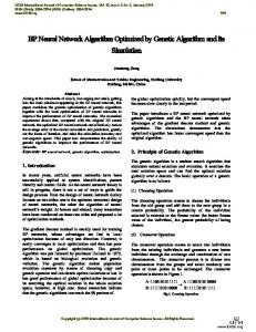
data. Despite the alluring prospect of data-driven methods, they are often criticized by hydrologists for the lack of physical hydrologic meanings and poor robustness. As a result, the integration of data-driving method and knowledge-based method may be an alternative way to overcome these problems. For this purpose, we proposed to combine artificial neural networks (ANNs) with the traditional hydrological model. ANNs have shown excellent characteristics in dealing with nonlinear systems [17,18]. Especially, ANNs using back propagation algorithm in training phase scilicet BP-ANNs [19], which has been accepted as a major forecasting method in reservoir operation, water quality classification, and water resource planning [20,21]. If learning data are sufficient, it can accurately reproduce the target results [22,23]. However, they also suffer from some drawbacks [24]. For instance, there is no standardized way of selecting network architecture [25]. The error of a single moment can hardly be eliminated as ANNs lack physical meaning [26]. Further, the accuracy of prediction by ANNs declines as the leading time increases. An incorporation of ANNs into current hydrological model may solve these problems. River channel flow calculations are important to hydrological modeling and flood forecasting. It is especially true for the distributed hydrological modeling which becomes a general consensus of today [27]. The outflow of each sub-basin needs to be routed along a river channel to the outlet of the watershed and their concentration times are quite different. The calculation errors in upper channel segments will accumulate and be enlarged in the simulations in lower channel segment. To obtain more accurate flood forecasting, it is necessary to estimate the errors of the river channel flow calculation. Many factors could influence the results of river channel flow calculation such as the errors of runoff, rainfall, etc. Previous studies have applied BP neural network algorithm for correcting runoff, etc. [14]. Moreover, for increasing number of sub-basins or fully distributed hydrologic model, it will cost a high computational demand to apply BP neural network algorithm. Therefore, e channel routing for updating is considered more realistic for distributed and semi-distributed hydrological models. To simplify the model construction, we focus on the local inflow errors of the main river channel instead of those of all river channels. In this study, we applied the Back-propagation Neural Network Correction (BPC) method to the semi-distributed Xinanjiang model to update the local inflows for Muskingum channel routine calculations for main river channel. We aim to take advantages of capability of data-driven methods and knowledge-based method to provide a more accurate flood forecasting system. 2. Study Area and Data The Dingan River is located in the central region of Hainan Island in southern China. It is one of the major inputs to Wanquan River. Dingan River watershed is less affected by the water conservancy project as a headwaters area. The climate is dominated by tropical monsoon system with annual average temperature at 22 ◦ C. The average annual precipitation is about 1639 mm, of which 70% is derived from typhoons and summer rainy season. The precipitation has a strong seasonal variability. About 70% to 90% of precipitation occurs during the period from May to November, which poses a great challenge on flood control. In this paper, hourly rainfall data were collected in 11 rainfall stations in the Dingan River watershed (Figure 1). The corresponding observed hoult streamflow data were collected at Jiabao station at the outlet of the watershed. The digital elevation model (DEM) with a spatial resolution of 90 m is collected for sub-basin division. The watershed is selected because it is not disturbed by major water conservancy projects. Moreover, the data quality is good for both precipitation and streamflow with no missing value.
Water 2017, 9, 48 Water 2017, 9, 48 Water 2017, 9, 48
3 of 16 3 of 16 3 of 16
Figure 1. Distribution of hydrological stations network in Dingan River watershed. Figure 1. Distribution of hydrological stations network in Dingan River watershed. Figure 1. Distribution of hydrological stations network in Dingan River watershed.
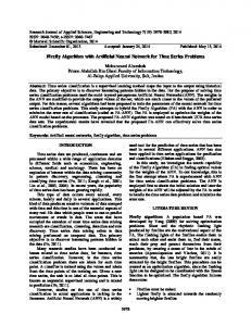
3. Methods 3. Methods 3. Methods 3.1. BP Neural Networks 3.1. BP Neural Networks 3.1. BP Neural Networks BP neural network is a typical multilayer ANN, and uses Back-propagation to train the BP neural network is a typical multilayer ANN, and uses Back‐propagation to train the network BP neural network is a typical multilayer ANN, and uses Back‐propagation to train the network network [28]. The common structure used in hydrology to map all continuous nonlinear function [28]. The common structure used in hydrology to map all continuous nonlinear function consists of [28]. The common structure used in hydrology to map all continuous nonlinear function consists of consists of three layers: input layer, hidden layer, and output layer (Figure 2). A neural network three layers: input layer, hidden layer, and output layer (Figure 2). A neural network is composed of three layers: input layer, hidden layer, and output layer (Figure 2). A neural network is composed of is composed of with massive nodes, with thresholds, activation functions weights and connection weightsthe to massive nodes, with thresholds, activation functions and connection connection weights to characterize characterize the massive nodes, thresholds, activation functions and to characterize the architecture of the network [29]. The BP algorithm is a supervised learning method architecture of of the the network network [29]. [29]. The The BP BP algorithm algorithm is is a a supervised supervised learning learning method method based based on on the the architecture based on the steepest descent method to minimize the global error. The output errors are fed back steepest descent method to minimize the global error. The output errors are fed back through the steepest descent method to minimize the global error. The output errors are fed back through the through the network to modify the threshold values and connection weights. Finally, the optimal network to modify the threshold values and connection weights. Finally, the optimal value can be network to modify the threshold values and connection weights. Finally, the optimal value can be value can be obtained via iterative adjustment. Objective function takes root mean square error. obtained via iterative adjustment. Objective function takes root mean square error. obtained via iterative adjustment. Objective function takes root mean square error.
Figure 2. Configuration of a three-layer BP neural network. Figure 2. Configuration of a three‐layer BP neural network. Figure 2. Configuration of a three‐layer BP neural network.
The neural network used in this paper has three layers and the number of nodes in hidden layer The neural network used in this paper has three layers and the number of nodes in hidden layer is The neural network used in this paper has three layers and the number of nodes in hidden layer is determined by means of “trial and error”. It first employs the initial value calculated by Equation determined by means of “trial and error”. It first employs the initial value calculated by Equation (1) is determined by means of “trial and error”. It first employs the initial value calculated by Equation (1) and then less and more nodes are conducted to find the best performing one as the final value (1) and then less and more nodes are conducted to find the best performing one as the final value expressed as [30]: expressed as [30]:
Water 2017, 9, 48
4 of 16
and then less and more nodes are conducted to find the best performing one as the final value expressed as [30]: Number of nodes in the hidden layer = (input number + output number) ×
2 3
(1)
The activation function of output layer is linear while the remaining layers are sigmoid functions. The outputs are obtained corresponding to the value of inputs using the formula as follow: Qk =
m
n
j =1
i =1
∑ Vjk × F ∑ pi × Wij + boj
!
+ bhk , k = t, t + 1, · · · , N
(2)
where Wij is the connection weight between ith node in the input layer and jth node in the hidden layer; Vjk is the connection weight between jth node in the hidden layer and kth node in the output layer; bo and bh are the bias, namely the threshold value, of nodes in the output layer and hidden layer respectively; Pi is the input of ith node; n, m and N are the number of nodes in the input layer, hidden layer and output layer, respectively; and F is the activation function of the hidden layer and in this paper is sigmoid function. Various improved algorithms exist for building a BP neural network model [31–33]. In this study, three improved algorithms are selected: (1)
Momentum factor application [26,34]
The application of momentum factor is conducive to avoid oscillation when excessive correction happens and to speed up training on occasion it encounters flat regions of the error surface. The biases and corresponding connection weights are adjusted based on the following formula: ∆Wij (n) = − β
bi ( n ) = − β
∂E(n) + η∆Wij (n − 1) ∂Wij
(3)
∂E(n) + ηbi (n − 1) ∂bi
(4)
where Wij is the connection weight between the ith node of preceding layer to jth node of this layer; n is the training times; E is the simulation error; β is the learning rate; η is the momentum factor; and bi is the threshold value of ith node of this layer. (2)
Learning rate adaptation [35]
Real-time adjustment of learning rate of the network is essential to accelerate convergence. This paper selects the multiple of interval (2,5) of the distance from the calculation error to the target and interval (0.25,5) of the initial learning rate to construction proportional function, choosing the integer multiple of distance to form the double ratio coefficient array. When the multiple of distance is beyond the interval, it equals to the boundary value. The specific calculated function is expressed as follow: k12 β 0 , E(n) ≤ k11 Edis k22 β 0 , k11 Edis ≤ E(n) < k21 Edis β(n) = ········· k (m−1)2 β 0 , k (m−1)1 Edis ≤ E(n) < k m1 Edis k m2 β 0 , k m1 Edis ≤ E(n)
(5)
where n is the training times; Edis is the target error; E is the current calculation error; β0 is the initial learning rate; km1 is the mth double ratio coefficient to the target error; and km2 is the corresponding learning rate correction factor to the km1 . km1 and km2 increase with the increase of m. The bigger is the double ratio coefficient of km1 , the faster the learning rate of the next training phase becomes.
Water 2017, 9, 48
(3)
5 of 16
Crossing validation [36,37]
Crossing validation is conducted to avoid over fitting by determining when the neural network begin to over-train. Over fitting happens when the neural network tries to fit the noise component of the data. Under this circumstance, it performs well over the training dataset, but shows poor results in forecasting. To apply the crossing validation, the data coverage period should be partitioned into three periods: calibration period (to calibrate the model parameters of the neural network), validation period (to stop the calibration phase when over training happens), and verification period (to test the accuracy of the simulation results). If the available dataset is too small for partitioning, the recommend solution is to stop the training when the objective error ceases to decrease significantly. 3.2. BP Neural Network Correction Algorithm 3.2.1. Traditional BP Neural Network Correction Algorithm The traditional BP neural network correction algorithm is based on the principle of error auto regression. It is validated by the supervised learning method which requires actual value of variables to guide the training process. The inputs are the forecast error information of past N time periods, thus the real-time forecast error is calculated by the following equation: et = Q p,t − Qo,t
(6)
et+ L = FBP (et , et−1 , · · · , et− N +1 )
(7)
Q0p,t+ L = Q p,t+ L − et+ L
(8)
where et is the calculation error at t moment; Q p,t is the calculated value at t moment; FBP (·) is the BP neural network method and its inputs; and Q0p,t is the corrected calculated value at t moment. In real-time correction, error autocorrelation in neighboring moment is at its strongest compared with each period. Therefore, prediction accuracy would decline as leading time increase. Intermediate variables such as sub-basin runoff yield and local inflow of main river channel generalized cannot be corrected by this method. 3.2.2. The Hydrological Model The XAJ model chosen in this paper is a semi-distributed rainfall–runoff model developed in 1992 [38]. It is a typical conceptual hydrological model; the main feature of the model is the concept of runoff formation on repletion of storage. It means that, after the soil moisture context of aeration zone of the entire basin reaches field capacity, the runoff equals the rainfall excess. XAJ model has been proven as an effective model to simulate runoff in humid and semi-humid region. It has been applied over a large area including almost all of major river basins in China [39,40]. The study watershed is divided into eleven sub-basins and runoff of each sub-basin is computed. The outflow of each sub-basin (local inflow) is routed down the main river channel to the entire basin outlet concentrated by the Muskingum method. River concentration time of sub-basin in different positions is quite different. The outflow of upstream has a significant impact on the prediction results of downstream. Thus, we focus on the concentration part of XAJ model choosing the local inflow of main stream to be updated to improve the accuracy of flood forecasting. 3.2.3. Apply BPC Algorithm in the Model Considering that m channel segments of main river channel have local inflow, the inputs of BPC are the observed discharge and simulated discharge by XAJ model. The outputs are the estimated local inflow calculated errors of m channel segments of L hour ago. Then, Muskingum calculation process of L hours was repeated using the corrected local inflow. The calculation process can be expressed as follow (Figure 3):
Water 2017, 9, 48
6 of 16
Qm ,t -L FBPC (Q p ,t , Qo ,t ) Water 2017, 9, 48
(9)
Q p ,t FMSJG ( Qm ,t L , Qm ,t L )
Q o ,t
6 of 16
(10)
Q
p ,t is the calculated discharge after is the observed discharge at t moment; ∆Qm,t−L = FBPC ( Q p,t , Qo,t ) (9) Qm ,t Muskingum at t moment; FBPC () is the BPC method and its inputs; is the estimated error Q0p,t = FMSJG (∆Qm,t−L , Qm,t− L ) (10) Q m ,t of local inflow of mth channel segment calculated by BPC; is the uncorrected local inflow of where Qo,t is the observed discharge at t moment; Q p,t is the calculated discharge after Muskingum mth channel segment calculated by XAJ at t moment; FMSJG () is the Muskingum method and its at t moment; FBPC (·) is the BPC method and its inputs; ∆Qm,t is the estimated error of local inflow of Q p ,t mth channel calculated by local BPC; inflow Qm,t is of themth uncorrected local inflow mth channel inputs; and segment is the corrected channel segment at t ofmoment after segment L hours 0 is the calculated by XAJ at t moment; F (·) is the Muskingum method and its inputs; and Q MSJG p,t recalculation of Muskingum. corrected local inflow of mth channel segment at t moment after L hours recalculation of Muskingum.
where
Divide the sub‐basins
Calculate the Muskingum river confluence
Traditional hydrological model
Calculate the outflow of each sub‐basin to obtain the local inflow of each channel segment (Qm,t) of main river channel at t moment
The discharge calculated after Muskingum at t moment Qp,t
The observed dischage at t moment Qo,t
Main river confluence by Muskingum Recalculate the Muskingum river confluence for L hours Q'p,t
Calibrate the neural network by the supervised learning method to obtain the estimated errors of each channel segment L hours ago △Qm,t‐L to update the Qm,t‐L
BP‐ANN Meet the requirement? Cycle >Max cycle times or RMSE(Q'p,t ‐Qo,t )