Design Methodology to trade off Power, Output Quality and Error Resiliency: Application to Color Interpolation Filtering Georgios Karakonstantis, Nilanjan Banerjee, Kaushik Roy, & Chaitali Chakrabarti2 Purdue University1 , West Lafayette, USA Arizona State University2, Tempe, USA {gkarakon,nbanerje,kaushik}@purdue.edu
[email protected]
Abstract: Power dissipation and tolerance to process variations pose conflicting design requirements. Scaling of voltage is associated with larger variations, while Vdd upscaling or transistor up-sizing for process tolerance can be detrimental for power dissipation. However, for certain signal processing systems such as those used in color image processing, we noted that effective trade-offs can be achieved between Vdd scaling, process tolerance and “output quality”. In this paper we demonstrate how these tradeoffs can be effectively utilized in the development of novel low-power variation tolerant architectures for color interpolation. The proposed architecture supports a graceful degradation in the PSNR (Peak Signal to Noise Ratio) under aggressive voltage scaling as well as extreme process variations in sub-70nm technologies. This is achieved by exploiting the fact that some computations are more important and contribute more to the PSNR improvement compared to the others. The computations are mapped to the hardware in such a way that only the less important computations are affected by Vdd-scaling and process variations. Simulation results show that even at a scaled voltage of 60% of nominal Vdd value, our design provides reasonable image PSNR with 69% power savings. 1. Introduction Present-day integrated circuits are expected to deliver highperformance under ever-diminishing power budgets. Poweraware designs are necessary to prolong the battery lifetime of portable devices, to prevent excessive heat generation which could affect device reliability, and to reduce the cost associated with expensive cooling techniques. One of the power reduction techniques, namely, supply voltage scaling [1], increases the delays in all computation paths and can result in incorrect or incomplete computation of certain paths. Therefore, applying supply voltage scaling indiscriminately to any design can adversely affect the output, leading to lower manufacturing/parametric yield. Besides power dissipation, process variations also pose a major design concern with technology scaling. Studies in [2] have shown that parameter variations create a delay spread of almost 30% for 70 nm process technology, leading to delay failures in some chips. Proposed techniques such as scaling and gate upsizing come at a cost of increased power and/or die area. Hence, meeting the conflicting requirements of high yield, low power and high quality is becoming exceedingly challenging in nanometer designs. We propose a system-level approach to handling the conflicting requirements by jointly considering optimizations at the algorithm as well as the architecture levels. At the algorithm level, we utilize the fact that for certain DSP applications, such as those used in color image processing, all computations are not equally important in shaping the output response; some computations are critical for determining the output quality,
while others play a less significant role. This information can be exploited to develop suitable algorithm/architecture that provide the right trade-off between output quality, energy consumption (supply scaling) and parametric yield due to process variations. The proposed design approach is shown in Fig. 1. In the first step, we identify the critical/non-critical components of such systems based on output sensitivities. Next, the complexity is minimized by modifying the components that contribute less towards improvement of quality. When the quality requirements are satisfied, the modified algorithm is mapped to the architecture such that the important components are not affected under Vdd scaling and/or delay failures due to process variations. By adopting this technique, we obtain low-power and variation-aware architectures where a “reasonable” output quality is maintained. In this paper, we demonstrate the use of this methodology in the design of a novel low power, variation-tolerant architecture for color interpolation. Color interpolation is the process used in color image processing for reconstruction of missing color samples in each pixel location. This is one of the most critical and computationally demanding operations in the image processing chain of a digital camera. Further more, because of portability considerations, the power consumption of this unit should be kept low. Thus the design requirements of the interpolation module are that it should consume low power and yet maintain a reasonably high Peak Signal to Noise Ratio (PSNR). We tackle the contrasting issues of low-power, variationtolerance and high quality for the color interpolation module by introducing innovations at the algorithm/architecture level. We begin by identifying crucial/less-crucial computations for maintaining high output image PSNR in color interpolation. We present a Vdd-scalable/variation-tolerant architecture where crucial computations are computed with higher priority. This S pe cifica tions : D e sig n to trad e off P ow er, O utp ut Q u a lity a nd P roce ss T olera nce , set q ua lity m etric A lg orith m ic le ve l: D eterm in e com po n en ts tha t co ntrib ute sig n ifican tly to qu ality M in im ize co m plexity by m o difying com p on en ts th at ha ve le ss im p act o n qu ality
no
A ccep tab le Q ua lity a t m inim a l o verh ea d ? ye s
A rch itec tura l le v el: M a p m o dified a lg orithm g iving priority to m ore im p o rtan t co m po ne nts A ccep ta ble qu a lity u nd er V d d sca ling an d/o r p ro cess variatio ns?
no
ye s
L ow P ow er P roce ss A w a re H ig h Q ua lity A rchite cture
Fig. 1: The design methodology
B1,-1
B-1,-1 G-1,0 B-1,1 G0,1 G0,-1 Ri,j B1,1 G1,0
m=0
n=0
Fig. 2: Bayer CFA pattern
allows a gradual degradation in PSNR with Vdd-scaling (low power) and/or delay variations. In fact, unlike existing implementations [3], our architecture can operate even under a scaled-supply voltage of 60% of nominal Vdd (for 70 nm CMOS technology) while maintaining “reasonable” PSNR. To the best of our knowledge, this is the first time that the problem of developing scalable color interpolation architecture has been addressed. It should be noted that the basic methodology proposed in this paper is equally applicable to a large class of signal processing applications where trade-offs between quality/power-dissipation/yield is required. The rest of the paper is organized as follows. The proposed voltage scalable algorithm design methodology is presented in Section 2. Section 3 presents a detailed description of the proposed low power/process tolerant architecture along with simulation results. Section 4 concludes the paper. 2. Color interpolation: Principles and Design In this section, we briefly present the essentials of conventional color interpolation schemes. We then identify the critical/less-critical components in color interpolation and present a new algorithm for variation-aware low power color interpolation. 2.1 Fundamentals Each pixel of a color image consists of 3 primary color channels, red (R), green (G) and blue (B), and hence, imaging systems require 3 image sensors – one for each color channel. However, due to cost constraints, it is customary for such devices to capture an image with a single sensor, sample only one of the three primary colors at each pixel and then store them in color filter arrays (CFA). In order to reconstruct a full color image, the missing color samples at each pixel location need to be interpolated by a process called color interpolation. The Bayer pattern [4] (Fig. 2) is the most frequently used CFA interpolation pattern and consists of R, G and B channels. Interestingly, the Bayer pattern contains twice as many G channels as compared to R and B channels. 2.2 Determination of critical components Bilinear interpolation [4] is the basic building block for all color interpolation schemes. In this method, the missing color values at each pixel are determined using the average of the adjacent pixels of the same color. For instance, if we want to interpolate the missing values of the color channels, G and B at the red pixel Ri,j, we compute the average of neighboring G and B values (Fig. 2): ∧
G
i, j
=
1 4
∑
∧
(G i + m , j + n ) , B
( m , n ) = {( 0 , − 1 ), ( 0 , 1 ), ( − 1 , 0 ), ( − 1 , 0 )}
i, j
=
1 4
∑
in estimating that missing color (G) at the other pixel locations (R and B). The bilinear method can therefore be identified as an integral part of all interpolation algorithms. To improve interpolation accuracy and obtain better image quality, more advanced techniques [5] have been developed that exploit the correlation among R, G, B channels or the edge direction information to adaptively interpolate each of the missing colors. In [6], missing colors are estimated by applying bilinear interpolation to the color difference domain G-R and GB to obtain superior image quality. In edge sensing methods [7, 8], the interpolation methods are adjusted to estimate the pixels along edge directions and not across them. More sophisticated methods [9,10] have been proposed that can lead to further PSNR improvement by using results from B and R interpolation to correct G interpolation, and vice versa. However, these complex techniques either require excessive hardware for their implementations or require additional software processing for practical realization. Therefore, attaining high image PSNR requires careful consideration of both edge sensing and pixel correlation. We propose an effective scheme, in which we divide the computations required for interpolation into two parts based on their impact on the output image quality. The first part consists of the bilinear component which is absolutely necessary for interpolation, and the second part consists of a correction term needed to improve image PSNR. The correction term is designated as “gradient” and is defined as a 2-D vector of an image intensity function I(x,y), with the components given by the derivatives in the horizontal and vertical direction at each image pixel [11]. The quality improvement from the gradient computation is termed gradient correction. The contribution of the bilinear and gradient computation terms for the image Sail is presented in Fig.3. Both the bilinear and the gradient computations can be perceived as 2-D filtering. In Fig 4(a), the coefficient values for bilinear computation are shown in green with weights {2, 2, 2, 2}, and the remaining 5 coefficients are for gradient computation and shown in red with values {4, -1, -1, -1, -1}. The gradient is zero in regions of constant pixel intensities and so the sum of the coefficients for gradient computation is always equal to zero [9]. Filtering is done on the entire image using the sliding window protocol. The window size is typically 5x5 or 7x7 depending of the performance and filtering requirements. 2.3 Proposed Design Methodology for Low Power/Variation Aware Design After the determination of the critical/less-critical components, the computations are restructured to enable
( B i+ m , j+ n )
( m , n ) = {( − 1 , − 1 ), ( − 1 , 1 ), ( 1 , − 1 ), ( 1 , 1 )}
Although this method results in low PSNR, it is widely used due to its simplicity. Also, due to significant spatial correlation among image pixels, the information contained in the neighboring pixels (say neighboring G’s) is extremely important
(a) (b) (c) Fig. 3: Image results (a) Original, (b) Bilinear (28dB), (c) Gradient correction (7.495dB)
2
2
-1
4
2
2
-1
b
a
4
6
2
2 -3/2
c a
5
c
a
4
5 4
a
b
-1
2
2
-1
a d
b
-1 On B pixel
-1
-3/2 2 -3/2
6
2
5
a
4
c
-3/2 2 -3/2
2
c
a
2
4
2
On G pixel
f
a d
4
a
-3/2
2 2
a On R pixel
-1
-3/2
-1
4 a f
5
4
a
b
On G pixel
a d
a
4
a
a
d
f f R row, B column R column, B row (c) (a) (d) (b) Fig 4: Color interpolation of: (a) G and B values at R pixel, (b) R and B values at G pixel, (c) G and R values at B pixel, (d) R and B values at G pixel -3/2
efficient mapping onto the variation-aware low-power architecture. The basic idea is to retain the bilinear component in all computations and vary the size and complexity of the gradient component. At nominal Vdd, the filter windows and coefficients used in our design are similar to that proposed in [12], since these set of coefficients yield extremely high PSNR with less design complexity. In [10], the authors determine the coefficient values based on optimal Weiner criterion [11] for a 5x5 interpolation window. Under scaled voltages and parameter discrepancies, the delays in all computation paths increase. To maintain reasonable image quality under such a scenario, we reduce design complexity by varying the values and the number of coefficients for gradient computation. The new filter coefficients are suboptimal in Wiener criterion. However, by performing a rigorous error analysis we attempt to minimize the error imposed after each alteration of the coefficient values/numbers. We also ensure that the coefficients for gradient computation always sum up to zero. 2.3.1 Nominal Vdd Fig. 4 shows the different filter windows utilized for interpolation of missing colors at nominal Vdd. For a row consisting of R and G pixels, Fig 4(a) and 4(b) shows the coefficients for estimation of G and B values at the R pixel and R and B values at the G pixel, respectively. Similarly, for a row consisting of G and B pixels, Fig. 4(c) and 4(d) show filter coefficients for calculating G and R values at the B pixel and R and B values at the G pixel, respectively. We distinguish between the computation of R and B values at the G pixel on an R-G row to that of R and B values at the G pixel on a G-B row. In spite of the differences, the same hardware can be used to determine both the computation sets just by switching two inputs for the second case. Similarly, the computation of G and B values at the R pixel (Fig. 4(a)) and G and R values at the B pixel (Fig. 4(c)) are identical, with just the red and the blue pixels interchanged. The similarities in the computations are used to optimize the hardware and have been described in more detail in Section 3. Mathematically, the filter operation for the interpolation of G value at the R pixel (Fig. 4(a)) at nominal supply voltage is given by the following expression: ∧ (1) G i, j = 2∑ (Gi + m, j + n ) ( Ri + m, j + n ) + 4( Ri , j ) /8 ∑ ( m , n ) ={( −2, 0 ),( 2, 0), ( 0, −2), ( 0, 2 )} ( m,n )={( −1, −1),(1,−1),( −1,1),(1,1)} Similar expressions can be derived for the other filters. The coefficient values of these filters are shown in Fig. 4. Note that all computations in Fig. 4 are divided by 8 to obtain the correct estimated pixel values. Prediction of missing colors at a pixel location through color interpolation introduces some error in the processed image. In
order to show the effectiveness of our approach, we perform an error analysis at nominal Vdd by estimating the mean square error (MSE). We evaluate the error value for two distinct cases: 1) Homogeneous window: In a homogenous region, the R, G, B pixels are highly correlated and the pixels have similar intensity values as shown in Fig. 5(a). For instance, Fig. 5(a), shows a homogeneous region consists of pixels with high intensity values denoted by H. This essentially implies that there are no sudden edges present within the interpolation window. 2) Window with Edge: Here the region of interpolation is not homogenous and there are edges in it. Fig. 5(b) shows a vertical edge, where H and L denote the high and low intensity values, respectively. Similarly, a window can consist of edges of type horizontal or diagonal. Next we show how error computations are done for the filters under consideration. For every interpolation window, we compute the error ∆ = |Pi,j – P’i,j|, where Pi,j and P’i,j are the pixel values of the original and the reconstructed image, respectively. For instance, the error for computing the R value at the G pixel (Fig. 5a) is calculated as follows: ∆R,Nominal-Homogeneous= |Pi,j,orig –Pi,j’nominal |= |( 8HR – (8 HR + (5+2c+4a+2b)HG )/8| = (5+2c+4a+2b) HG/8 where Pi,j = HR (pixel frequency in original image) and Pi,j’ is the reconstructed R channel by using filter shown in Fig. 4(b). After substituting the coefficient values a=b=-1 and c=1/2 in the above equation, the error in the homogenous region is ∆R,Nominal-Homogeneous= ((5+2*1/2 -4 -2) HG)/8 = 0 The error for the region with vertical edges (Fig. 5(b)) is ∆R_Nominal-Edge= (8HR –(4(HR +LR)+(5+b+2a+2c)HG + +(b+2a)LG))/8| = (4(HR - LR)-3 (HG - LG))/8 = (4((LG- LR)-(HG- HR)) + (HG - LG))/8 = (HG - LG)/8 In the above error computation we assume (LG- LR)≈(HG- HR), since it has been shown in [6] that differences LG-LR and HG-HR have similar values over a small interpolation region. For sake of brevity, we show the analysis for only one filter of Fig. 4(a). However, identical analysis can be easily performed for other filters shown in Fig. 4. The estimated error, ∆R_Nominal is used to evaluate the performance of our approach after Vdd scaling, as described in the following section. 2.3.2 Scaled Vdd
b
a a
4 c
c 5
a
4
a
Filter Region
b
HG HR HG HR HG HB HG HB HG HB HG HR HG HR HG HB HG HB HG HB HG HR HG HR HG (a)
b
a a
4 c
c 5
a
4
a
b
HG HR HG L R LG HB HG HB LG LB HG HR HG LR LG HB HG HB LG LB (b) HG HR HG LR LG
Fig. 5. (a) Homogeneous region, (b) Vertical edge
-1
2
2 -21
2
2
-1
-1
-1 4 4
-1 -1
4 On G pixel
On R pixel
-1
2 2
2
2
2 -1 (a)
-1
-1 4 4 1 4
--11 (b)
Fig 6: Filter window for the computation of (a) G and B values at R pixel, (b) R, B values at G pixel under scaled voltage Vdd1
At scaled voltages, we alter the number and values of coefficients for computing the gradient. In this subsection, we first describe each of the filters for estimating the missing pixel values for two scaled voltages (Scaled voltage1) and (Scaled voltage2) and analyze their impact by analytically evaluating the errors at those voltages. The values of the scaled voltages are determined from architectural design considerations. In our design, we have considered two cases: i) nominal Vdd scaled by 20% (Vdd1) and ii) nominal Vdd scaled by 40% (Vdd2). The choice of these voltage values for performing color interpolation is explained in detail in section 3. Scaled voltage1: To design an architecture which meets the delay constraints at a reduced voltage Vdd1, we reduce the number of operations and hence the critical path of the design by changing the filter size from 9 to 7 for G and B computations at the R pixel, and from 11 to 7 for R and B computations at the G pixel. Similar filter size reduction holds for the other four cases. The corresponding filters are shown in Fig. 6. The new filters retain the coefficients for the bilinear computation as in the nominal Vdd case, and certain terms for gradient computation so that there is minimal PSNR degradation. It should also be observed that the remaining filter coefficients constituting the gradient component are altered to make their sum equal to zero. Similar to the previous error analysis (R at G pixel), we obtain ∆R,ScaledVdd1= |(8HR – (8 HR + (4+4a’)HG )/8| = (4+4a’) HG/8=0. If a’=-1, ∆R,ScaledVdd1-Homogeneous= (4-4) HG)/8 =0. In case there is a vertical edge, ∆R,ScaledVdd1-Edge=| (HG-LG)/4|. Scaled Voltage2: We further scale the supply voltage to Vdd2< Vdd1. At this voltage, for the computation of the G and B values at the R pixel, we obtain only the bilinear component. For the computation of the R and B values at the G pixel, we obtain the bilinear component and a simplified gradient component as shown in Fig. 7. Similar to the previous error analysis (R at G), we obtain: ∆R,ScaledVdd2 = (1+a”) HG/8, where a”= -1 Therefore, ∆R,ScaledVdd2-Homogeneous = (1-1) HG)/8 = 0 The worst case error in case there is a vertical edge is given by ∆R,ScaledVdd2-Edge = |3(HG-LG)/8| The magnitude of this error is this case is high due to further 2
2 -1 2
2
4
-1 1
2
2 2
(a)
R G B image
3.6 3.24 3.09 3.41
4.36 3.24 3.09 3.89
2.59 1.41 1.95 2.37
0.62 0 0.29 0.41
reduction of filter window size. Fig. 8 shows the image results for the original as well as the processed image at nominal and scaled Vdds. It is interesting to note that even when the supply is scaled to as much as 0.4 times it nominal value, we still obtain results with better PSNR values than one that uses only bilinear interpolation. 2.4. Experimental results To verify the effectiveness of our approach, we applied the filters corresponding to Vdd1 and Vdd2 on a set of 25 Kodak images and compared the results with the nominal Vdd case and the signal correlation method [6]. Table 1 presents the average PSNR for R, G, B color channels and the whole image. At nominal Vdd, our method produces better results than signal correlation. For scaled voltage Vdd2, we do not obtain any improvement for the G channel compared to the bilinear case. But due to the improvement in the R and the B channel values, the performance of our approach at scaled voltage Vdd2 is better than bilinear interpolation at nominal Vdd. We compare the design complexity of our method with a popular algorithm [6], where the color interpolation method using signal correlation required 20 additions to estimate 2 missing pixel values. Our method on the other hand requires 31 additions to compute 4 missing color channels. Therefore at nominal Vdd our method provides higher PSNR at lower computational complexity. 3. Implementation of Scalable Architecture In this section, we first propose a method for improving the performance of color interpolation by almost a factor of two with negligible area overhead. Next, we present our voltagescalable variation-resilient architecture based on the voltage scalable algorithm presented in Section 2. 3.1. Architectural innovation for high throughput In the sliding window based approach, the filter window traverses the entire image and so the size of the filter determines the speed of interpolation. In conventional color interpolation, the filter is of size 5x5; one pixel location is targeted at a time and the interpolation of the two missing pixel values at that location is computed. As shown in section 2, the calculation of the R and B values at the G pixel is different from the computation of the G and B values at the B pixel. However, we
4 On G pixel
On R pixel
2
Table 1: Average PSNR (dB) improvement over bilinear interpolation for the 25 images for each color channel and the whole image Sig. Nominal Scaled Scaled Channel Corr. Vdd Vdd1 Vdd2
4
1
4 -1
(b)
Fig. 7: Filter window for the computation of (a) G and B values at R pixel, (b) R, B values at G pixel under Vdd2
(a) (b) (c) (d) Fig. 8: Sail Image (a) Original, (b) Nominal, (c) at Vdd1 (d) at Vdd2
note that the filtering of R and B values at the G pixel on an RG row differs slightly from that of R and B values at the G pixel on a G–B row (Fig. 4). As shown in Section 2.3.1, it is possible to utilize the same hardware just by interchanging the R and B inputs depending on the row that is being traversed. Therefore hardware implementation of the filters of Fig. 4(a) and (b) are adequate to perform color interpolation at all pixels depending on the row it is operating on. We take advantage of the significant overlap between the filtering requirements of two adjacent pixels in a row and propose to utilize a window of size 5X6 pixels for interpolation. For instance, it is possible to interpolate missing values at 2 adjacent pixel locations in a row (either for R and G in R-G rows, or G and B in the G-B rows) at the same time without any hardware overhead. Hence, by using a 5x6 window, we obtain twice the throughput (e.g. B and G at R along with R and B at G) if the filter window is chosen to be 5x6 instead of 5x5. 3.2. Scalable Architecture for color interpolation Fig. 9 shows the scalable architecture for estimating the G and B values at R pixel (Fig. 4(a)) and R and B values at G pixel (Fig. 4(b)) for the G-B row. We analyze the architecture under i) Vdd scaling and ii) process variations. 3.2.1 Vdd scaling The proposed architectures, shown in Fig. 9, maximizes the sharing between the computations of G and B values at the R pixel and R and B values at the G pixel and thus reduces the hardware requirements. For instance, while computing the G and B values at the R pixel, we find that the summations of the Ri,j terms are identical and they differ only with respect to the scaling factors. This aspect is utilized in effectively sharing the hardware and is highlighted in Fig. 9(a). Also in each of the computations, the bilinear portion is computed first so that it does not get affected by Vdd scaling/process discrepancies. For instance, in case of G and B computations at the R pixel, the bilinear component is computed after the 2nd adder, labeled as ab2 in Fig. 9(a), and in R and B computations at the G pixel, it is computed after the 1st adder, abil2 in Fig. 9(b). Instead of scaling the output by 1/8, we scale the inputs by shifting 3 bits. This
G’●1
ab2
V dd
G’ 2 ●
Vdd M1 ―
G’i,j
M
G’3
B’●1
Vdd M1
Ri−2, j ― Ri+2, j ……………………………….… >>3 Ri, j-2 ― Ri, j+2 ― >>2
Vdd nominal Vdd
B’2
>>3
M
●
>>1
>>1
abil2 ― V dd M1 a1
V2
R’●1
>>3
a2
V dd
R’2
B’i,j
B’3
Overlapping computations
Bi-1, j Bi+1, j Gi−1, j−1 Gi, j
>>3 >>1
M
●
R’i,j
R’3
a3
―
a4
Critical path
………………………………….. Vdd nominal V1 >>1
>>3
― Vdd M1
V2
B’●1
.………………….….…....
>>2
>>3
……………………………
>>2 Ri, j >>1
V1
V2
………........………...........
…………… ………......…
………………………………..
Gi, j
………………………………….. Vdd nominal V1
Gi+1, j−1 >>3 ― Gi−1, j+1 ― >>3 Gi+1, j+1 …………………………………. Gi, j+2 >>3 Gi,j−2 ― >>4 Gi−2, j Gi+2, j
―
Ri, j -2 Ri, j+2 ………………………………….. Ri+2, j Ri -2, j Bi−1, j−1 Bi−1, j+1 Bi+1, j−1 Bi+1, j+1
Ri, j-1 Ri, j+1 Gi−1, j−1
.………………….….…....
>>2
Vdd nominal
……………………………
>>2 >>1
V1
V2 ab1
……………………………...
Ri, j
……………………………...
Gi−1, j Gi, j−1 Gi+1, j Gi, j+1
………………………….………
helps in reducing the bit-width of the adders. At nominal Vdd, the frequency of operation is determined by the maximum of the critical path delays for all the computations. In this design, the maximum delay occurs in the computation of R and B values at the G pixel (Fig 9(b)). It is 4 adders + 1 three-input multiplexer + 1 two-input multiplexer, noted as Tcri=D(M1)+D(a1)+D(a2)+D(a3)+D(a4)+D(M), where D(i) is the delay in module i. The worst case delay in the computations in Fig 9(a) is (Tcri – D(M1)), which is comparable to Tcri since the delay in M1 is quite small. The voltage scaling signals, V1 and V2 serve as control signals to the 3-input multiplexer and determine the appropriate output at nominal/scaled voltages. At nominal Vdd, both the voltage scaling signals, V1 and V2 are set to zero. Operation at scaled voltage, Vdd1 is achieved by setting the control signal V1=’1’. At this voltage, the computation of Tcri can no longer be completed. However, if the voltage is scaled such that the computation of M1+a1+a2+a3+M is valid, the multiplexer chooses the middle input in each of the computations. We explain the operation using the computation of the R value at the G pixel as an example. At Vdd1, the multiplexer chooses R’2 as shown in Fig. 9(b). In order that the coefficients for the gradient component have equal positive and negative weights, we add a multiplexer, M1, to choose between ½ and ¼ for Gi,j as shown in Fig. 9(b). Further voltage scaling (Scaled Vdd2) is obtained by setting the value of the second control signal V2 = ‘1’. The multiplexer chooses the top input in each of the computations. For instance, for the computation of the R value at the G pixel, the multiplexer chooses R’1 as shown in Fig. 9(b). The delay in this case is D(M)+D(a1)+D(a2)+D(M), and it dictates the minimum voltage to which the design operates correctly. At Vdd2, the output for the G and B values at the R pixel consists of only the bilinear component. The output for the R and B values at the G pixel consists of the bilinear component (output of a1) and a small gradient. Again, the input multiplexer M1 chooses the scaled values to satisfy the zero gradient requirements. The extra hardware required to incorporate the scaled Vdd/process-aware option for all the 4 outputs consists four (8bit) 3-input multiplexers at the output and two 2-input
Gi+1, j−1 >>3 ― Gi−1, j+1 ― >>3 Gi+1, j+1 …………………………………. Gi, j+2 >>4 Gi,j−2 Gi−2, j ― >>3 Gi+2, j
Vdd
B’ 2 ●
M
B’i,j
B’3 ―
Overlapping
computations (a) Fig. 9: Proposed Architecture for the interpolation of (a) G and B values at R pixel, (b) R and B values at G pixel
(b)
Table 2: Power consumption (mW) and PSNR (dB) for the Sails image for three values of operating voltages Nominal Vdd (1V) V1(0.8V) V2 (0.6V) Vdd P (V) PSNR P (V) PSNR P (V) PSNR Proposed 13.2 38.15 7.8 35.25 3.67 32.9
multiplexers at the input. We implemented the proposed architecture in VHDL and synthesized it using Synopsys Design Compiler. The architecture was simulated in HSpice using BPTM 70 nm technology using 1000 patterns and the average power consumption was determined. The results for power consumption and the image PSNR, under nominal and scaled Vdds are shown in Table 2. Note that even when we scale Vdd by 40%, adequate PSNR is obtained. The obtained results are in accordance with the estimated errors, presented in section 2. The overall area overhead is 2% and the power overhead at nominal Vdd is 3%. 3.2.2 Process tolerance We also investigated the impact of process variation on our architecture at nominal and scaled voltages. At nominal voltages, parameter variations might affect the delays in computations, which are in the slower process corners. In such a scenario, the output at the 4th adder (a4 in Fig. 9(b)) would be incomplete or invalid. However, with the help of a process sensor [13], we can easily detect the process corner and correspondingly set the first Vdd control signal V1 to ‘1’. This will slightly degrade the quality of the image at nominal Vdd, but will provide a valid output. At scaled Vdds (say Vdd1), because of parametric variations, the computation of the 3rd adder (a3 in Fig 9(b)) might not be complete. In that case, we can set V2=’1’ and obtain a valid output at the expense of quality of the image. We use HSpice to perform statistical simulations on our design assuming a transistor threshold voltage spread of 30% (70 nm technology), to determine the lowest voltage, where we can obtain a valid output under severe parameter disparities. We observe that we obtain bilinear output at a scaled voltage of 0.6V (where nominal is 1V at 70 nm technology) under severe process variations. It is evident that the proposed platform generates color interpolation designs that are tailored to provide 100% manufacturing yield under parameter discrepancies by allowing trade-offs between quality and yield. For our architecture we consider two distinct cases: i) At nominal supply voltages, the output PSNR of the image of color interpolation chips (at the worst case process corner) are minimally affected as only the “gradient” values have errors in computation, ii) At worst case process corners under scaled voltages, we still obtain a graceful degradation of image quality since the gradient values are affected at first. Of course, beyond a certain voltage (< 0.6* nominal Vdd), quality degrades rapidly since the bilinear computations experience delay failures. 3.3 Measurement Results Table 3: Measurement Results from Xilinx Spartan-3 FPGA Nominal Vdd Vdd1 Vdd2 Vdd (0.9V) (0.8V) (0.7V) Proposed 59.5 mW 40.8 mW 30.1 mW
Table 4: Xilinx device occupancy Method
Slices
LUT
Equivalent gates
Proposed Existing [8 ]
258 518
484 795
2985 10068
We mapped the above architecture onto a Xilinx Spartan-3 FPGA to verify its functionality and also to obtain the power results. For the power measurements, the voltage regulator was disconnected and power was supplied to the core. The power values for the three implementations are shown in Table 3. We note that we get significant power reduction by operating at scaled voltages. Table 4 tabulates the FPGA occupancy. A recently proposed low-power color interpolation design in [6] requires two divisors, three multipliers, and seven adders and 2 line buffers. The increased complexity of this design is apparent from the results shown in Table 4. 4. Conclusion We have developed a novel design methodology, where intelligent trade-offs between power, quality and error resiliency is utilized to simultaneously achieve low energy and variationtolerance, while maintaining a reasonably high quality response. The design methodology has been applied to digital signal processing, in particular, to a color interpolation filter. The basic concept behind this approach is to constrain the components that contribute more to the output quality to the initial computation stages, and the less important ones to the later stages. Such a structuring enables graceful degradation of output quality even when the design is subjected to voltage scaling and process variations. References [1] J. Rabaey et al., “Digital Integated Circuits”, Prentice Hall, 2002 [2] S. Borkar et al., “Parameter variations and impact on circuits and microarchitecture”, DAC 2003, pp. 338–342. [3] B. K. Gunturk et al., "Demosaicking: color filter array interpolation," IEEE Signal Process. Mag. 22(1), 44–54 , Jan. 2005. [4] R. Ramanath et al., “Demosaicking methods for Bayer color arrays,” J. Electronic Imaging, vol. 11, pp. 306–315, July 2002. [5] J. E. Adams, Jr., “Design of practical color filter array interpolation algorithms for digital cameras,” Proc. SPIE, vol. 3028, pp. 117–125, Feb. 1997. [6] S.-C. Hsia, et al., “VLSI Implementation of low-power high-quality color interpolation processor for CCD camera”, vol 14, issue 4, pp. 361369, April 2006. [7] S.C. Pei, et al., “Effective color interpolation in CCD color filter array using signal correlation,” Proc. ICIP, pp. 488–491, Sept. 2000. [8] E. Chang, et al.., “Color filter array recovery using a threshold-based variable number of gradients,” Proc. SPIE, vol. 3650, pp. 36–43, Jan.1999. [9] R. Kimmel, “Demosaicing: image reconstruction from color CCD samples,” IEEE Trans. on Image Processing, vol. 8, pp. 1221–1228, Sept. 1999. [10] B. K. Gunturk et al., “Color plane interpolation using alternating projections”, Trans. on Image Processing, vol. 11, pp. 997–1013, Sept. 2002. [11] A Bovik, “Handbook of Image & Video Processing”, ISBN 0-12119790-5, Academic Press, San Diego, 2000. [12] H. S. Malvar et al., “High-quality linear interpolation for demosaicing of Bayer-patterned color images”, ICASSP, vol 3, pp. 485488, May 2004. [13] C.H. Kim et al., “On-die CMOS leakage current sensor for measuring process variation in sub-90nm generations”, Symp. of VLSI Circuits, 2004, pp.250-251.