Attribute Value Selection Based on Minimum Description Length
Istvan Jonyer JONYER@ACM .ORG Lawrence B. Holder
[email protected] Diane J. Cook
[email protected] Department of Computer Science and Engineering, University of Texas at Arlington, Box 19015, Arlington, TX 76019
Abstract We introduce a new method for attribute value selection, which is driven by the minimum description length principle. We demonstrate the viability of the approach on the Wisconsin breast cancer data set, show a working exa mple and evaluate the approach against earlier systems. Comparisons on different domains are also given. Empirical results show that our approach consistently outperforms competing machine learning algorithms on domains with all numeric, all discrete and mixed attributes types.
1.
A number of different approaches to attribute value selection exist. Information gain has been utilized in decision tree induction, regression and other statistical methods are used to build statistical models, and the list goes on. Even description length has been utilized for guiding the search for hypotheses (Cameron-Jones & Quinlan, 1994). To our knowledge, however, the MDL principle has not been applied directly to attribute value selection. In the next section we give background and further motivation for our research. We then describe the algorithm in detail followed by examples and experimental results. We conclude with a discussion of the results and directions for future work.
Introduction 2.
Attribute value selection is of central importance in data mining and machine learning algorithms for learning class hypotheses. When learning models, a learning algorithm must choose the attributes, and for each attribute, its values, to maximize the model’s performance according to some metric. Attribute value selection is concerned with selecting the values to be included for each attribute in a model. Selecting the best values for each attribute has a direct effect on the model’s performance. One well known benchmark is C4.5 (Quinlan, 1993) which uses information gain to order attributes and select attribute values to construct a decision tree. Other methods include linear discrimination (Wen-Hua, Madigan, & Scott, 2002), multi-surface separation (Wolberg & Mangasarian, 1990) and nearest neighbor (Zhang, 1992). Most of these are rooted in statistics, and are designed specifically for data sets with numeric attributes. C4.5 is one method that has employed information theory successfully while not restricted to numeric domains. This paper introduces a new method for attribute value selection, which is driven by the minimum description length principle (Rissanen 1989). We demonstrate the viability of the approach on the Wisconsin breast cancer domain, and show comparisons with earlier systems. We also show results on other domains which contain discrete attributes as well.
Attribute Value Selection Based on MDL
Our approach is based on an algorithm for discovering frequent substructures in graphs, called Subdue (Cook and Holder 2000). Subdue is based on information theory, and seeks to minimize the description length of the entire data set. We imagine an agent wishing to communicate a data set to its counterpart. One option is to convert the data to a bit stream, and send it. A better way might be to identify common parts in the data that may be abstracted out and sent separately. This way, at least that common pattern is not repeated needlessly. This is consistent with Occam’s razor, which states that “entities should not be multiplied without necessity.” Its modern interpretation is the minimum description length principle, which was introduced by Rissanen (1989). Subdue is able to identify static patterns in any input graph. It can also discover patterns that may vary in their structure from instance to instance by a user-defined threshold. Such a variance may also be applied to numeric vertex labels. The problem with discovering patterns in this way is that the user has to make a guess as to what amount of threshold will produce the best results. This work attempts to remove the need for tweaking a threshold while allowing for flexibility in the types of patterns to be learned. In this work we are not concerned with structural variances, only with varying values for attributes across instances of the learned pattern. For simplicity, we will refer to attributes with multiple values
as variables, as opposed to attributes with a single value to which Subdue was formerly restricted. In essence, we are looking to develop a way for Subdue to learn variables. Subdue is an algorithm that is especially well suited for learning in complex data sets, because it represents data as a graph. It can, however, handle flat, feature-vectorbased data sets just as well. Such databases can be represented as a graph by converting each feature vector into a star-like graph in which a central node serves as the anchor from which edges originate with attribute labels, and terminate in vertices having the attribute value as their label. Even though the results presented here apply to graphs of any degree of complexity, we chose to restrict our discussion to flat data sets for several reasons: (1) competing approaches typically work on flat data exclusively; (2) using flat data makes comparisons possible, and reported results by competitors on the same data is readily available in the literature; (3) there are more, readily available, popular data sets of this type; (4) the explanation may be easier to follow. To simplify the discussion, we use terminology that refers to features of the database, not its graph representation. Many techniques exist for selecting attribute values that are descriptive of one class and not the other. Linear and surface-based separation techniques can be useful but only in numeric domains, or where categorical values can be ordered naturally. Problems can still arise if the classes cannot be separated in such a manner, like in the case of a normal distribution where the negative class consists of outliers. Neural networks and nearest neighbor algorithms may overcome this, but human expertise is essential for good results. More sophisticated statistical methods can achieve better results, but they only work on numeric domains. Table 2 compares the performance of 15 such techniques on the Wisconsin Breast Cancer domain. Several considerations led us to experiment with using the MDL principle for selecting values for attributes. First, Subdue was already using this heuristic successfully, so it made sense to extend this approach to attribute values. A literature search revealed that the MDL heuristic has not been applied to this problem directly. In addition, the MDL approach has the advantage of being able to handle discrete attribute values as well as numeric ones. Since Subdue is a general purpose algorithm, this is an important point. The next section describes the algorithm in detail, including graph encoding, exact MDL computation, and an example. It also includes a discussion on the algorithm’s complexity.
3.
The Learning Algorithm
The learning algorithm works by performing a beam search for the hypothesis that minimizes the description length of the input data set. In a very high-level view, the algorithm considers each attribute and calculates the description length for each. The best attribute is selected and becomes a partial hypothesis. This partial hypothesis is successively extended by adding other attributes to it. To select the best attribute to add, all remaining attributes that are not in the hypothesis are recomputed as part of the hypothesis. The best attribute selected this time is likely to provide additional reduction in description length. If so, it is added to the hypothesis. This process continues until no more attributes can be added, or the best attribute does not provide a decrease in description length. Figure 1 shows the pseudo-code for the algorithm. But how are values selected for the attribute that minimizes the description length? The number of possible subsets of values for a given attribute is exponential. We can, however, apply the observation that the most reduction in description length is provided by values that occur more frequently. Hence, attribute values have a ranking based on their frequency. This ranking is local to each attribute over the positive examples. That is, it does not take into account negative instances, and does not assume anything about the global performance of each attribute value. This ranking, however, allows us to Subdue( graph G, int Beam, int Limit ) queue Q = { v | vertex v has a unique label in G } bestSub = first substructure in Q repeat newQ = {} for each substructure S in Q newSubs = ExtendSubstructure(S) newQ = newQ U newSubs Limit = Limit - 1 Q = substructures in newQ with top Beam MDL scores if best substructure in Q better than bestSub then bestSub = best substructure in Q until Q is empty or Limit 0) ∗ c +d (lg s + ∑ s * lg(ui − 1) ) i=1
[
]
rbits is the number of bits needed to encode the rows of the adjacency matrix A. To do this, we apply a variant of the encoding scheme used by Quinlan and Rivest
(Quinlan and Rivest 1980). This scheme is based on the observation that most graph representations of realworld domains are sparse. In other words, most vertices in the graph are connected to only a small number of other vertices. Therefore, a typical row in the adjacency matrix will have much fewer 1s than 0s. We define k i to be the number of 1s in row i of adjacency matrix A, and b = maxi (k i ) (that is, the most 1s in any row). An entry of 0 in A means that there are no edges from vertex i to vertex j, and an entry of 1 means that there is at least one edge between vertices i and j. Undirected edges are recorded in only one direction (that is, just like directed edges). If there is an undirected edge between nodes i and j such that i < j, then the edge is recorded in entry A[i, j] and omitted in entry A[j, i]. A flag is used to signal if an edge is directed or undirected, which is accounted for in ebits. rbits is calculated as follows. (1) Given that k i 1s occur in the ith row’s bit string of length v, only
v strings of 0s and 1s are possible. ki
Since all of these strings have equal probability of v occurrence, lg bits are needed to specify which ki combination is equivalent to row i. The value of v is known from the vertex encoding, but the value of k i needs to be encoded for each row. This can be done in lg(b + 1) bits. (2) To be able to read the correct number of bits for each row, we need to encode the maximum number of 1s any given row in A can have. This number is b, but since it is possible to have zero 1s, the number of different values is b + 1. We need lg(b + 1) bits to represent this value. Therefore,
v v rbits = ∑ lg(b + 1) + lg + lg(b + 1) i =1 ki v v = ( v + 1) lg(b + 1) + ∑ lg i=1 ki ebits is the number of bits needed to encode the edges represented by A[i, j] = 1. The number of bits needed to encode a single entry A[i, j] is (lg m) + e(i, j)[1 + lg le], where e(i, j) is the number of edges between the vertices i and j in the graph and m = maxi,j e(i, j)—the maximum number of edges between any two vertices i and j in the graph. The (lg m) bits are needed to encode the maximum number of edges between vertices i and j. For each edge we need (lg m) bits to specify the actual number of edges, and [1 + lg le] bits are needed per edge to encode the edge label and the directed flag (1 bit). The total number of edges is e, and K is the number of 1s in the adjacency matrix A. Therefore,
[
]
v v ebits = lg m + ∑ ∑ A[ i, j ](lg m) + e(i , j)[1 + lg le ] i=1 j=1 v v = lg m + e(1 + lg le ) + ∑ ∑ A[ i, j ] lg m i=1 j=1 = e(1 + lg le ) + ( K + 1) lg m
The description length of the graph G compressed by substructure S is DL(G) = DL(G|S) + DL(S) where DL(G|S) = vbits(G|S) + rbits(G|S) + ebits(G|S) DL(S) = vbits(S) + rbits(S) + ebits(S) The formula for computing the description length in concept learning given positive and negative inputs is DL(G+,G- ) = DL(G+|H) + DL(H) + DL(G- ) – DL(G- |H) where DL(H) is the description length of the hypothesis, G+ is the positive input set, G- is the negative input set, DL(G+|H) is the positive input set compressed by the hypothesis, DL(G- |H) is the negative input set compressed by the hypothesis, and DL(G+,G- ) is the positive and negative input sets compressed by the hypothesis. DL(H) + DL(G+|H) expresses the number of bits needed to encode the hypothesis plus parts of the positive input that are not described by the hypothesis. DL(G- ) – DL(G- |H) is the number of bits needed to describe the portion of the negative input that is described by the hypothesis. For the rationale behind this formula we refer back to our two agents wishing to communicate the database from one to another. As before, one needs to send the hypothesis H and the rest of the positive input that is not described by H. This can be done in DL(G+|H) + DL(H) bits. If H covers negative examples as well, one needs to communicate those examples as exceptions from our rule H. This requires DL(G- ) – DL(G- |H) bits, which is the part of the negative input that is covered by H. 3.2.
Example with Encoding Computation
In this section we give a working example for the algorithm and the above description length encoding calculation. We use the Wisconsin Breast Cancer database which is introduced in detail in section 4.1. We start by converting the database to graph representation. Each of its feature vectors are converted into a star-like graph with a center vertex out of which nine edges emanate for the attributes, terminating in nine vertices which represent the attribute values. For instance, the vector 7, 4, 6, 4, 6, 1, 4, 3, 1 translates to the graph shown in figure 2. For a less crowded appearance, we replaced the attribute names on the edges with numbers according to table 2. The positive input graph consists of 452 such graphs for each of the
benign cases, and the negative input graph consists of 241 graphs for the malignant cases. 4
6
4 3
2
7
1
6 4
5
Case
1 6
4
7
The adjacency matrix has 3290 rows, such that b = maxi (k i ) = 9. Therefore,
3290 3290 + (42) 9 6
rbits(G | S) = (3291)lg(1 0) + (410)
3
8 9
= 10932.4 + (410)(60.6 0) + (42)(86.67 )
1
= 39420.57
Figure 2. Graph representation of vector 7, 4, 6, 4, 6, 1, 4, 3, 1.
We start the example at the entry point of the SelectAttributeValues() function and execute the first iteration of the repeat-loop using a substructure that already has 2 attributes, as shown in figure 3. The vertex labels show the continuous value ranges selected for those attributes. [1..2]
Mitoses
Case
Uniformity of Cell Size
[1..2]
Figure 3. Graph representation.
The SelectAttributeValues() function is passed the substructure shown in figure 3 and the attribute Clump Thickness which has actual values ranging from 1 to 8. The function determines that the attribute is continuous, and computes its mean, which is 2.82. The attribute is added to the substructure using all its values (1..8). The next step is to evaluate this new substructure by calculating its description length. First, we compute the description length of the substructure (S). The table of vertex labels has 13 entries (“Case”, 10 integer values, and 2 floating-point numbers). Hence, lv = 13. S contains four vertices (v = 4), three continuous variables (c = 3), and no discrete variables (d = 0). Therefore, vbits(S) = lg 4 + 4(lg 13) + 4 + 3 + 0 + (3)lg 13 = 34.90 The adjacency matrix has 4 rows, such that k 1 = 3, k 2 = 0, k 3 = 0, k 4 = 0, b = maxi (k i ) = 3. Therefore, rbits(S) = (4 + 1)lg(3 + 1) + lg 4 = 12 The table of edge labels has the names of the nine attributes, so le = 9. There are three edges in the subgraph (e = 3), and the maximum number of edges between any two vertices is one (m = 1). There are a total of three ones in the adjacency matrix (K = 3). Hence, ebits(S) = 3(1 + lg 9) + (3 + 1)(lg 1) = 12.51 DL(S) = 23.80 + 12 + 12.51 = 59.41 Next we compute the description length of the positive input graph G+ compressed using substructure S. The number of vertices in the compressed input graph can be computed as the number of positive examples times number of vertices per example minus the number of vertices covered by S times number of instances covered by S plus number of instances covered by S. That is, v = (452)(10) – (410)(4) + 410 = 3290. The last term accounts for each vertex that was added to the graph in place of each substructure abstracted out. For the three continuous variables, u 1 = 2, u 2 = 2, u 3 = 8, while s = 410. vbits(G|S) = lg 3290 + 3290(lg 13) + ((3 + 0) > 0)(lg 410 + 1151.01) = 11.68 + 12174.45 + (1)(1159.69) = 13345.8
There are 410 graphs with 6 edges and 42 with 9 edges making e = 2838. The maximum number of edges between any two vertices is one (m = 1). There are a total of 2838 ones in the adjacency matrix (K = 2838). Hence, ebits(G|S) = 2838 (1 + lg 9) + (2839)(lg 1) = 11834.25 DL(G|S) = 13345.8 + 39420.56 + 11834.25 = 64600.61 We do not follow the computation for the negative graph since that is very similar to the previous calculations. Substructure S covers a single negative example. The total encoding comes to DL(G+,G- ) = 64939.54 bits. Continuing with our example, the SelectAttributeValues() function enters the repeat-loop. Since the attribute is continuous, the value farthest from the mean (2.82) is removed. This value is “8”, shrinking the attribute’s range to [1..7]. The evaluation results in DL(G+,G- ) = 64909.77 bits, which is slightly better than the previous substructure, so it becomes the new best substructure. The repeat-loop continues until all but one value remains in the attribute, at which point the function returns the best substructure that was created using the best set of values. 3.3.
Complexity
The algorithm has to select values for each of the a attributes Aj , each of which has v(Aj ) unique values. If the data set has s number of positive examples, then the upper bound on v(Aj ) is s. Computing the rank of values can be done in one pass. Selecting the values for all attributes is hence O(as). Since the partial hypothesis is extended a times (for a attributes), the upper bound is O(a 2 s).
4. 4.1.
Experiments The Wisconsin Breast Cancer Database
The Wisconsin breast cancer database was obtained from the University of Wisconsin Hospitals, Madison from Dr. William H. Wolberg, through the UCI Machine Learning Repository (Keogh, Blake & Merz, 1998). The data set contains description for 693 cases of breast cancer of two classes: 452 benign and 241 malignant cases. The data set has nine continuous numeric attributes—excluding the class attribute—with values as shown in table 2. A comparison table describing accuracies from various systems on the Wisconsin Breast Cancer domain reported in the literature is shown in Table 1. It lists predictive accuracies reported for each algorithm, which were obtained using 10-fold cross validation as reported by the sources cited in the right column. In our tests we used a
Table 1. Comparison with other approaches on the breast cancer domain.
Rank 1 2 3 4 5 6 7 8 9 10 11 12 13 14 15 1
Algorithm Probit RLP Gaussian Process Feature Minimization GSBE SVM Multi-surface separation (3 planes) 1 Subdue FOIL C4.5 Neural Networks 1-nearest neighbor 1 Multi-surface separation (1 plane) 1 Linear Discriminant Logistic regression
Accuracy 97.2% 97.07% 97.0% 96.92% 96.77% 96.7% 95.9% 95.67% 94.8% 94.4% 93.3–95.61% 93.7% 93.5% 92.9% 92.3%
These experiments worked with only 369 examples (200 training cases, tested on the other 169 cases).
90/10 split between training and test sets. As we can see, Subdue outperforms 7 out of 14 other systems, with an accuracy of 95.67%. The ones that do better are mostly statistical systems (such as RLP, GSBE, Gaussian process, multi-surface separation, etc.) specifically designed for continuous-valued domains. Even these are only 1.5% more accurate, at best. C4.5, a general-purpose system (i.e., one that also handles discrete-valued attributes) that is considered a benchmark in machine learning, did worse than Subdue, with only 94.4% prediction accuracy.
misclassification). Since this rule covers over 92% of all cases, it gives a good idea of how benign and malignant cases differ. A graphical depiction is shown in Figure 5. Benign cases are represented by the lower dark area. Rule 1: 1 = Clump Thickness = 8, AND 1 = Uniformity Of Cell Size = 2, AND 1 = Uniformity Of Cell Shape = 4, AND 1 = Marginal Adhesion = 10, AND 1 = Single Epithelial Cell Size = 5, AND 1 = Bare Nuclei = 5, AND 1 = Bland Chromatin = 7, AND 1 = Normal Nucleoli = 2, AND 1 = Mitoses = 2
Table 2. Breast cancer attributes.
# 1 2 3 4 5 6 7 8 9
Accuracy Reported by Wen-Hua et al, 2002 Brodley & Utgoff, 1995 Wen-Hua et al, 2002 Brodley & Utgoff, 1995 Brodley & Utgoff, 1995 Wen-Hua et al, 2002 Wolberg & Mangasarian, 1990 Authors Authors Liu & Setiono, 1996 Taha & Ghosh, 1997 Zhang, 1992 Wolberg & Mangasarian, 1990 Wen-Hua et al, 2002 Wen-Hua et al, 2002
Attribute Name Clump Thickness Uniformity of Cell Size Uniformity of Cell Shape Marginal Adhesion Single Epithelial Cell Size Bare Nuclei Bland Chromatin Normal Nucleoli Mitoses
Value Range 1 - 10 1 - 10 1 - 10 1 - 10 1 - 10 1 - 10 1 - 10 1 - 10 1 - 10
Aside from predictive accuracy, an algorithm is also judged by how simple it is for the human data miner to interpret its findings. Humans prefer systems that describe most of the data using small, simple rules. To see how Subdue fares at producing quality rules, we performed a classification task using all examp les for training and testing. Subdue terminated after finding 6 rules which describe benign cases with 98.12% accuracy. The best 2 rules achieved 96.39% accuracy. Figure 4 shows the textual description of the best rule that covers 399 benign cases and 1 malignant case (a
Figure 4. Rule #1 for the breast cancer domain.
$1 10$1 $1 $0
5-
$0 $0
11
2
3
4
5
6
7
8
9
Attributes
Figure 5. Graphical representation of rule #1 for the breast cancer domain.
4.2.
Effects of Data Skew
Concept learning in Subdue works by attempting to learn rules that describe the positive examples well while not describing any of the negative examples. That is, an example is classified as negative if the hypothesis found for the positive examples does not classify it as positive. Some systems, like C4.5, find hypotheses for both positive and negative classes. Since this is not the case with Subdue, the choice of positive versus negative examples may make a difference in the rules generated,
and their accuracy. Our experiments show that this is in fact the case. Table 3 shows the results in terms of predictive accuracy, rule complexity (average rule count), and time spent learning in all 10 runs of the cross validation.
breast cancer domain, where one expert may label malignant tumors as positive while others may pick benign as positive. 10$1
Table 3. Experiment result for switched class attributes.
$1 $1
5-
Positive Benign Malignant
Cases
Accuracy
452 241
95.67% 94.23%
Rule Count 5.8 10.8
$0
Run time (h:m) 0:18 2:01
As Table 3 shows, the average rule count almost doubled when malignant cases were presented as positive examples. Rule #4, depicted graphically in Figure 6, gives us an insight into what is happening. As the figure shows, cases are classified as benign only if all attributes have a value that falls within the dark strip in the middle. If malignant cases were to be described (i.e. value ranges above and below the dark stripe), two separate ranges were necessary for attributes 1, 2, 3, 5, 6, and 7. Subdue can only assign a single range per attribute per rule. In other words, when switching classes from positive to negative, the difference lies in having to learn outliers versus the central, contiguous ranges. Accuracy was also affected slightly which is due to the number of examples available in each class. There are 452 benign cases and only 241 malignant cases. The accuracy of the hypothesis is directly dependent on the number of positive examples. Running times also differed greatly. When benign cases were positive, the computation lasted 18 minutes, while it took over 2 hours to compute the rules when the class labels were switched. At present, there is no way for Subdue to automatically detect which class would be better handled as positive. The user simply has to try it both ways, unless some intelligence about the database is already available. The effects of data skew may also affect other learning algorithms. To test this, we performed an experiment on FOIL in which we swapped the positive and negative examples in the breast cancer domain. The results were actually reverse compared to Subdue. FOIL achieved a 94.8% accuracy using 11.7 rules on average when malignant cases were positive, while its performance slightly decreased to 94.23% using 10.1 rules on average when the examples were swapped. As we can see, swapping positive and negative examples had a smaller effect on FOIL’s performance, although FOIL needed significantly more rules to construct its hypotheses and was also less accurate than Subdue. Learning outliers versus central tendencies may be avoided in most cases, since experts tend to label their examples of interest as positive. Problems arise when the difference is not clear or arbitrary. This is the case in the
$0 $011
2
3
4
5
6
7
8
9
Attributes
Figure 6. Graphical representation of rule #4 for the breast cancer domain.
4.3.
Other Comparisons
We also evaluated Subdue on domains that have nonnumeric attributes. We were particularly interested in how Subdue compared against other systems that were specifically designed for relational domains. We selected FOIL (Cameron-Jones & Quinlan, 1994) and Progol (Muggleton, 1995), which are prominent inductive logic learning systems. Both have had great success in a wide variety of domains. We also wanted to know how our approach measures up against an algorithm that was designed for flat domains. For this we used C4.5. We selected the vote, diabetes and credit domains to serve as the basis for our comparison. The vote domain is the Congressional Voting Records Database available from the UCI machine learning repository. It contains only discrete-valued attributes, having values y, n, and u (for yes, no, and unknown). The diabetes domain is the Pima Indians Diabetes Database, which contains 7 continuousvalued attributes. The credit domain is the German Credit Dataset from the Statlog Project Databases, also available from the UCI repository. The credit data set contains 13 discrete and 7 continuous-valued attributes. Table 4. Comparison of Subdue, FOIL, Progol and C4.5.
FOIL Progol C4.5 Subdue
Vote 93.02% 94.19% 94.48% 94.23%
Diabetes 70.66% 63.68% 74.62% 70.94%
Credit 68.60% 63.20% 70.90% 71.30%
Predictive accuracies are shown in Table 4, which were generated using 10-fold cross-validation. As evident from the table, Subdue outperformed the two ILP systems in all three domains, and was the best on the credit domain. C4.5, however, did significantly better on the diabetes domain than the other three systems. We performed tests to determine the statistical significance of the difference in performance of the competing systems against Subdue. The results for the Vote domain, shown in table 5, indicate that all four algorithms performed quite similarly.
Confidence values indicate low statistical significance, especially when comparing Subdue and Progol. Tests for the Diabetes domain, shown in table 6, indicate that FOIL and Subdue performed almost identically, while both significantly outperformed Progol. C4.5 did even better. Tests for the Credit domain, shown in table 7, tell us that Subdue significantly outperformed both FOIL and Progol, while doing only slightly better than C4.5.
show results on relational domains and make comparisons to other systems in the near future. Another possibility for improvement is automation of the discovery of structural variances. As mentioned before, Subdue is able to consider such variation, but human input is required to define a threshold. We also plan on expanding the experimentation to include more domains and algorithms, and trying to determine when the MDL approach performs better or worse than other approaches.
Table 5. Significance tests for the Vote domain.
Subdue – FOIL Subdue – Progol Subdue – C4.5
∆ Error ± σ -1.21% ± 6.51% -0.05% ± 4.78% 0.25% ± 4.93%
Confidence 71.44% 51.22% 56.16%
Acknowledgment This research is partially supported by a Defense Advanced Research Projects Agency grant managed by the Air Force Rome Laboratory under contract F3060201-2-0570.
Table 6. Significance tests for the Diabetes domain.
Subdue – FOIL Subdue – Progol Subdue – C4.5
∆ Error ± σ -0.29% ± 9.76% -7.26% ± 8.81% 3.68% ± 9.88%
Confidence 53.58% 98.58% 86.51%
Table 7. Significance tests for the Credit domain.
Subdue – FOIL Subdue – Progol Subdue – C4.5
5.
∆ Error ± σ -2.70% ± 4.99% -8.10% ± 4.63% -0.40% ± 4.88%
Confidence 93.94% 99.98% 59.93%
Discussion and Conclusions
In this paper we introduced an algorithm for selecting attribute values based on description el ngth for both discrete and continuous attribute types. We described the algorithm in detail, showed the encoding computation and illustrated it with an example. We used the Wisconsin breast cancer database to show the viability of the approach and compared it with other systems reported in the literature. Subdue outperformed 7 of 14 systems cited among which were general purpose machine learning algorithms. The systems that did better than Subdue used mainly statistical approaches that can only handle numerical domains. Using this domain we also showed that Subdue produces rules of high quality that are simple and describe much of the data. We also evaluated our algorithm using three other domains that had discrete-valued attributes as well. Using this data set as the basis for comparison, we compared our system against yet another set of algorithms. Subdue came out as the one that performed consistently well across all three domains among systems capable of relational learning. Even though we carried out our explanation of the algorithm using flat domains exclusively, the approach works just as well in relational domains. We have plans to
References Brodley, C.E. & Utgoff, P.E. (1995). Multivariate Decision Trees. Machine Learning, Volume 19 (1), pages 45–77. Cameron-Jones, R. M., & Quinlan, J. R. (1994). Efficient Topdown Induction of Logic Programs. SIGART Bulletin. Vol. 5, 1:33-42. Cook, D. J. & Holder, L. B. (1994). Substructure Discovery Using Minimum Description Length and Background Knowledge. In Journal of Artificial Intelligence Research, Volume 1, pages 231-255. Evaluation / Characterization of Classification Algorithms. Statlog Project, Universidade do Porto. http://www.liacc.up.pt/ML/statlog/ Keogh, E., Blake, C. L. & Merz, C. J. (1998). UCI Repository of machine learning databases [http://www.ics.uci.edu/~mlearn/MLRepository.html]. Irvine, CA: University of California, Department of Information and Computer Science. Liu, H. & Setiono, R. (1996). A probabilistic approach to feature selection: A filter solution. In Proceedings of the Thirteenth International Conference on Machine Learning. Morgan Kaufmann. Muggleton, S. (1995). Inverse Entailment and Progol. New Generation Computing Volume 13 245-86. Quinlan, J.R. (1993). C4.5: Programs for machine learning, Published by Morgan Kaufmann Publishers, London, England. 1993. Rissanen, J. (1989). Stochastic Complexity in Statistical Inquiry. World Scientific Publishing Company. Taha, I. & Ghosh, J. (1997). Evaluation and ordering of rules extracted from feedforward networks. In Proceedings of the IEEE International Conference on Neural Networks, pages 221–226. Wen-Hua, J., Madigan, D., & Scott, S. (2002). On Bayesian Learning of Sparse Classifiers. Avaya Labs Research. Wolberg, W.H. & Mangasarian, O.L. (1990). Multisurface method of pattern separation for medical diagnosis applied to breast cytology. Proceedings of the National Academy of Sciences, Volume 87, pages 9193–9196. Zhang, J. (1992). Selecting typical instances in instance-based learning. In Proceedings of the Ninth International Machine Learning Conference pages 470–479.