AUTOMATED GOAL-ORIENTED ERROR CONTROL I: STATIONARY VARIATIONAL PROBLEMS MARIE E. ROGNES∗ AND ANDERS LOGG∗† Abstract. This article presents a general and novel approach to automated goal-oriented error control in the solution of nonlinear stationary finite element variational problems. The approach is based on automated linearization to obtain the linearized dual problem, automated derivation and evaluation of a posteriori error estimates, and automated adaptive mesh refinement to control the error in a given goal functional to within a given tolerance. Numerical examples representing a variety of different discretizations of linear and nonlinear partial differential equations are presented, including Poisson’s equation, a mixed formulation of linear elasticity, and the incompressible Navier– Stokes equations. Key words. finite element method, a posteriori, error control, dual problem, adaptivity, automation AMS subject classifications. 65N30, 68N30
1. Introduction. When solving mathematical models using computer simulation, it is pivotal that the quality of the computed solutions may be determined. However, the assessment of the quality of a computed solution is challenging, both mathematically and computationally. As a consequence, the quality of the solution must often be assessed manually by the scientist or engineer running the simulation. This approach is unreliable as well as time-consuming, and it effectively prevents computer simulation from realizing its full potential as a standard tool in science and industry. For finite element discretizations, classic a posteriori error analysis provides a framework for controlling the approximation error measured in some Sobolev norm, cf. [1]. Over the last two decades, goal-oriented error control has been developed as an extension of the classic a posteriori analysis [9, 12]. Based on the solution of an auxiliary linearized adjoint (dual) problem, one may estimate the error in a given goal functional. This allows the construction of adaptive algorithms that target a simulation to efficient computation of a specific quantity of interest. Although the framework developed in [9, 12] is applicable to any nonlinear finite element variational problem in theory, a certain level of expertise is required to derive an error estimate for a particular problem and to implement the corresponding adaptive solver. In particular, the derivation of the dual problem involves the linearization of a possibly complicated nonlinear problem, and both the derivation and evaluation of the a posteriori error estimate remain nontrivial (at least in practice). As a result, goal-oriented error control remains a tool for experts. In this work, we seek to automate goal-oriented error control. By this we mean to automatically compute state-of-the-art error estimates and indicators with a minimal amount of input and expert knowledge. This has the potential of rendering goaloriented error control fully accessible to non-experts. More precisely, we consider a ∗ Center
for Biomedical Computing at Simula Research Laboratory, P.O. Box 134, 1325 Lysaker, Norway (
[email protected],
[email protected]). This work is supported by an Outstanding Young Investigator grant from the Research Council of Norway, NFR 180450. This work is also supported by a Center of Excellence grant from the Research Council of Norway to the Center for Biomedical Computing at Simula Research Laboratory. † Department of Informatics, University of Oslo, Norway. 1
2
MARIE E. ROGNES AND ANDERS LOGG
general variational problem of the following form: find u ∈ V such that F (u; v) = 0 ∀ v ∈ Vˆ ,
(1.1)
where F : V × Vˆ :→ R is a semilinear form (linear in v) on a pair of trial and test spaces (V, Vˆ ). We here present a general adaptive algorithm that seeks to find an approximate solution uh ≈ u of the variational problem (1.1) such that |M(u) − M(uh )| ≤ ǫ, where M : V → R is a given goal functional and ǫ > 0 is a given tolerance. The input to our adaptive algorithm is the semilinear form F , the functional M, and the tolerance ǫ. Based on the given input, the adaptive algorithm automatically generates the dual problem, the a posteriori error estimate, and attempts to compute an approximate solution uh that meets the given tolerance for the given functional. The generated error estimates are intimately connected to the dual-weighted residual estimates for stationary variational problems, such as those presented by Becker and Rannacher [9]. However, the challenges arising from the automation aspect and the strategies devised to tackle these challenges are novel; we do not know of any other existing approaches of this kind. In this paper, we limit the discussion to stationary variational problems. The question of automated error control for time-dependent problems will be considered in later works. 1.1. Outline. The outline of this paper is as follows. Our notation is introduced in Section 2. In Section 3, we present the goal-oriented error estimation framework for linear variational problems. The linear setting is discussed first for the sake of clarity. The extension to the nonlinear case is presented in Section 6. Our approach requires an automated strategy for the computation of error estimates and indicators. Such a strategy is presented in Section 4. Further, the evaluation of the error estimates rely on a dual approximation; a strategy for extrapolating an improved dual approximation is described in Section 5. The full adaptive algorithm is summarized in Section 7. The algorithm outlined has been implemented in a prototype module of the DOLFIN library [28], and some of the key aspects of the implementation are discussed in Section 8. In Section 9, we apply the presented framework to three examples: the Poisson equation, a three-field mixed formulation for the linear elasticity equations, and the stationary Navier–Stokes equations. Finally, we conclude and discuss further work in Section 10. 2. Notation. Throughout this paper, Ω ⊂ Rd denotes an open, bounded domain with boundary ∂Ω. We will generally assume that Ω is polyhedral such that it can be exactly represented by an admissible, simplicial tessellation Th . The boundary will typically be the union of two disjoint parts, denoted ∂ΩD and ∂ΩN . In general, the notation V (X; Y ) is used to denote the space of fields X → Y with regularity properties specified by V . If Y = R, this argument is omitted. For L2 (K; Rd ); that is, the space of d-vector fields on K ⊆ Ω in which each component is square integrable, the inner product reads h·, ·iK , and the norm is denoted || · ||K . If K = Ω, the subscript is omitted. For m = 1, 2, . . . , H m (Ω) denotes the space of square integrable functions with m square integrable distributional derivatives. 1 Also, Hg,Γ = {u ∈ H 1 (Ω), u|Γ = g}. Similarly, H(div, Ω) denotes the space of square integrable vector fields with square integrable divergence. Note that both the gradient of a vector field and the divergence of a matrix field are applied row-wise.
AUTOMATED GOAL-ORIENTED ERROR CONTROL I
3
A form a : W1 × · · · × Wn × V1 × · · · × Vρ → R, written a(w1 , . . . , wn ; v1 , . . . , vρ ), is (possibly) nonlinear in all arguments preceding the semi-colon, but linear in all arguments following the semi-colon. 3. A framework for goal-oriented error control. In this section, we present a general framework for goal-oriented error control for conforming finite element discretizations of stationary variational problems. The framework is a summary of the paradigm developed in [9, 12]. For clarity, we restrict our attention to linear variational problems and linear goal functionals. Extensions to nonlinear problems and nonlinear goal functionals are made in Section 6. Let V and Vˆ be Hilbert spaces of functions or fields defined on a domain Ω ⊂ Rd for d = 1, 2, 3. In this section, we consider the following linear variational problem: find u ∈ V such that a(u, v) = L(v)
∀ v ∈ Vˆ .
(3.1)
We assume that a : V × Vˆ → R is a continuous, bilinear form, and that L : Vˆ → R is a continuous, linear form. We shall further assume that the problem is well-posed; that is, there exists a unique solution u that depends continuously on any given data. The variational problem defined by (3.1) will be referred to as the primal problem and u will be referred to as the primal solution. Let Th be an admissible simplicial tessellation of Ω (to be determined) and assume that Vh ⊂ V and Vˆh ⊂ Vˆ are finite element spaces defined relative to Th . The finite element approximation of (3.1) then reads: find uh ∈ Vh such that a(uh , v) = L(v)
∀ v ∈ Vˆh .
(3.2)
We assume that the spaces Vh and Vˆh satisfy an appropriate discrete inf–sup condition such that a unique discrete solution exists. The problem (3.2) will be referred to as the discrete primal problem and uh the discrete primal solution. Relative to the approximation uh , we define the (weak) residual r(v) = L(v) − a(uh , v).
(3.3)
Some remarks are in order. First, r is a bounded, linear functional by the continuity and linearity of a and L. Second, as a consequence of the Galerkin orthogonality implied by Vˆh ⊂ Vˆ , the residual vanishes on Vˆh . In other words, r(v) = 0 ∀ v ∈ Vˆh .
(3.4)
We are interested in estimating the magnitude of the error in a given goal functional M : V → R. For a given tolerance ǫ > 0, we aim to find (Vh , Vˆh ) such that the corresponding finite element approximation uh , as defined by (3.2), satisfies η ≡ |M(u) − M(uh )| ≤ ǫ.
(3.5)
In addition, we would like to compute the value of the goal functional M(uh ) efficiently, ideally using a minimal amount of work. To estimate the magnitude of the error M(u) − M(uh ), we introduce the (weak) dual problem: find z ∈ V ∗ such that a∗ (z, v) = M(v)
∀ v ∈ Vˆ ∗ ,
(3.6)
4
MARIE E. ROGNES AND ANDERS LOGG
where (V ∗ , Vˆ ∗ ) is the pair of dual trial and test spaces, and a∗ denotes the adjoint of a; that is, a∗ (v, w) = a(w, v). We shall refer to z solving (3.6) as the dual solution. We assume that the dual test and trial spaces are chosen such that u−uh ∈ Vˆ ∗ and z ∈ Vˆ . This holds if Vˆ ∗ = V0 = {v − w : v, w ∈ V } and V ∗ = Vˆ . Combining (3.6), (3.3), and (3.1), we find that M(u) − M(uh ) = a∗ (z, u − uh ) = a(u − uh , z) = L(z) − a(uh , z) ≡ r(z). The error M(u) − M(uh ) is thus equal to the (weak) residual r evaluated at the dual solution z. By the Galerkin orthogonality (3.4), we obtain the following error representation: M(u) − M(uh ) = r(z) = r(z − πh z).
(3.7)
Here, πh z ∈ Vˆh is an arbitrary test space field, typically an interpolant of the dual solution. An identical error representation is obtained for nonlinear variational problems and nonlinear goal functionals with a suitable definition of the dual problem. We return to this issue in Section 6. It follows that if one can compute (or rather approximate) the solution of the dual problem, one may estimate the size of the error by a direct evaluation of the residual. However, some concerns remain that require special attention. First, the error representation (3.7) is not directly useful as an error indicator. The derivation of an a posteriori error estimate and corresponding error indicators from the error representation has traditionally required manual analysis, typically involving some form of integration by parts and a redistribution of boundary terms (fluxes) over cell facets. Second, for (3.7) to give a useful estimate of the size of the error, care must be taken when solving the dual problem (3.6). In particular, the error representation evaluates to zero if the dual solution is approximated in Vˆh . Finally, the derivation of the dual problem may involve the differentiation of a nonlinear variational form. We discuss how each of these issues can be automated in the subsequent sections. 4. Automated derivation of error estimates and error indicators. Starting from the error representation (3.7), one may derive a posteriori error estimates and error indicators that, loosely speaking, express the error in terms of the strong residual of the original partial differential equation and the lack of higher-order regularity of the finite element approximation. For instance, for Poisson’s equation −∆u = f and its corresponding variational problem defined by a(u, v) = hgrad u, grad vi and L(v) = hf, vi on V = Vˆ = H01 (Ω), one obtains r(z) = L(z) − a(uh , z) = hf, zi − hgrad uh , grad zi X X = hf, ziT − hgrad uh , grad ziT = hf + ∆uh , ziT + h−∂n uh , zi∂T T ∈T
=
X
T ∈T
hf + ∆uh , ziT + h[−∂n uh ], zi∂T ,
T ∈T
where [−∂n uh ] denotes an appropriate redistribution of the flux over cell facets. Several choices are possible, see for example [1, Chap. 6], but we here make the simplest possible choice and distribute the flux equally. In particular, we define [∂n uh ]|S = 12 (grad uh |T · n + grad uh |T ′ · n′ ) over all internal facets S shared by two
5
AUTOMATED GOAL-ORIENTED ERROR CONTROL I
cells T and T ′ , and [∂n uh ]|S = ∂n uh |S on external facets (facets on the boundary of Ω). Hence, one may estimate the error by |M(u) − M(uh )| ≤
X
ηT ,
(4.1)
T ∈T
where the error indicator ηT is given by ηT = |hf + ∆uh , z − πh ziT + h[−∂n uh ], z − πh zi∂T |.
(4.2)
We note that although one may in principle use ηT = |hf, ziT − hgrad uh , grad ziT | as an error indicator (without integrating by parts and redistributing the normal derivative), that indicator is much less efficient than the error indicator defined in (4.2). Both indicators will sum up to the same value (if taken with signs), but only as a result of cancellation. The error indicator (4.2) is generally smaller in magnitude, scales better with mesh refinement, and gives a sharper error bound when summed without signs. See [38] for an extended discussion. 4.1. A generic residual representation. Estimates similar to (4.1) have been derived by hand (originally for use with norm-based error indicators) for a variety of equations. A non-exhaustive list of examples includes standard finite element discretizations of the Poisson equation [3], various mixed formulations for the Stokes equations and stationary Navier–Stokes equations [37], H(div)-based discretizations of the mixed Poisson and mixed elasticity equations [10, 30], and H(curl)-based discretizations for problems in electromagnetics [7]. Duality-based goal-oriented error estimates have been derived for a number of applications, including ordinary differential equations [13], plasticity [33], hyperbolic systems [21], reactive compressible flow [36], systems of nonlinear reaction–diffusion equations [14, 35], eigenvalue problems [17], wave propagation [4], radiative transfer [34], nonlinear elasticity [24], the incompressible Navier–Stokes equations [8, 18], variational multiscale problems [23], and multiphysics problems [22]. These estimates share a common factor, namely that the error is expressed as a sum of contributions from the cells and the facets of the mesh. We demonstrate below that for a certain class of variational problems, one may automatically compute a residual representation of the following generic form: r(v) =
X
hRT , viT + hR∂T , vi∂T =
X
hRT , viT + [hR∂T , vi∂T ],
(4.3)
T ∈Th
T ∈Th
where [hR∂T , vi∂T ] =
X
S⊂∂T ∩Ω
1 (hR∂T , v|T iS + hR∂T ′ , v|T ′ iS ) + 2
X
hR∂T , viS .
S⊂∂T ∩∂Ω
It follows that one may use as error indicators ηT = |hRT , z − πh ziT + [hR∂T , z − πh zi∂T ]|.
(4.4)
Comparing with (4.2), we note that for Poisson’s equation, the cell and facet residuals are given by RT = f + ∆uh and R∂T = −∂n uh respectively.
6
MARIE E. ROGNES AND ANDERS LOGG
Fig. 4.1. The bubble function bT .
4.2. Automatic computation of the residual representation. We shall focus our attention on a class of residuals r satisfying the following assumptions: A1 (Global decomposition) The residual is a sum of local contributions: X rT . r(v) = T ∈Th
A2 (Local decomposition) Each local residual rT offers a local decomposition: rT (v) = hRT , viT + hR∂T , vi∂T
∀ v ∈ Vˆ |T .
(4.5)
A3 (Polynomial representation) The residual contributions are piecewise polynomial: RT ∈ P p (T ),
R∂T |S ∈ P q (S)
∀ S ∈ ∂T
∀ T ∈ Th ,
p, q ∈ N.
We note that A1 is satisfied if the bilinear and linear forms a and L are expressed as integrals over the cells and facets of the tessellation Th . We also note that A2 is satisfied if the variational problem (3.1) has been derived by testing a partial differential equation against a test function and (possibly) integrating by parts to move derivatives onto the test function. Assumption A3 is more restrictive and we shall discuss the implications of this assumption in more detail below. If assumptions A1–A3 are satisfied, one may automatically compute the residual representation (4.3) for a given variational problem (3.1). In particular, one may directly compute the cell and facet residuals RT and R∂T by solving a set of local problems on each cell T of the tessellation Th . If only assumptions A1–A2 are satisfied, one may automatically compute projections of the residual decomposition terms and hence an approximate residual representation. p To compute the cell residual RT , let {φi }m i=1 be a basis for P (T ) and let bT denote the bubble function on T . We recall that for a simplex T ⊂ Rd , the bubble function bT is defined by bT =
d+1 Y
λTxi
i=1
where λTxi is the barycentric coordinate function on T associated with vertex xi (the ith linear Lagrange nodal basis function on T ). Note that bT vanished on the boundary of T . See Figure 4.1 for an illustration. Testing the local residual rT against bT φi ,
AUTOMATED GOAL-ORIENTED ERROR CONTROL I
7
T. Fig. 4.2. The cone function βS
we obtain the following local problem for the cell residual RT : find RT ∈ P p (T ) such that hRT , bT φi iT = rT (bT φi ),
i = 1, . . . m.
(4.6)
To obtain a local problem for the facet residual R∂T , we define for each facet S on T the cone function βST by βST =
Y
λTxi ,
(4.7)
T i∈IS
where IST is a suitably defined index set such that βST |f ≡ 0 on all facets f of T but S. For an illustration, see Figure 4.2. Clearly, βST |S = bS . Next, let {φi }ni=1 be a basis for P q (T ). Testing the local residual rT against βST φi , we obtain the following local problem for each facet residual: find R∂T |S ∈ P q (S) such that hR∂T |S , βST φi iS = rT (βST φi ) − hRT , βST φi iT
∀ i ∈ IST .
(4.8)
We prove below that by assumptions A1–A3, the local problems (4.6) and (4.8) uniquely define the cell and facet residuals RT and R∂T of the residual representation (4.3). One may thus compute the residual representation (4.3) by solving a set of local problems on each cell T . First, one local problem for the cell residual RT , and then local problems for the facet residual R∂T restricted to each facet of T . If the test space is vector-valued, the local problems are solved for each scalar component. We emphasize that the computation of the residual representation (4.3) and thus the error indicator (4.4) may be computed automatically given only the variational problem (3.1) in terms of the pair of bilinear and linear forms a and L. In particular, the derivation of the error indicators does not involve any manual analysis. We remark that the local problems (4.6) and (4.8) are different from the local problems that were introduced in [6] to represent the cell and facet residuals RT and R∂T as a single residual. 4.3. Solvability of the local problems. To prove that the local problems (4.6) and (4.8) uniquely determine the cell and facet residuals, we recall the following result regarding bubble-weighted L2 -norms. For a proof, we refer to [1, Theorems 2.2, 2.4].
8
MARIE E. ROGNES AND ANDERS LOGG
Lemma 4.1. Let T be a d-simplex and let bT denote the bubble function on T . There exist positive constants c and C, independent of T , such that c||φ||2T ≤ hbT φ, φiT ≤ C||φ||2T
(4.9)
for all φ ∈ P p (T ). We may now prove the following theorem. Theorem 4.1. If assumptions A1–A3 hold, then the cell and facet residuals of the residual representation (4.3) are uniquely determined by the local problems (4.6) and (4.8). Proof. Consider first the cell residual RT . Take v = bT φi in (4.5) for i = 1, . . . , m. Since v vanishes on the cell boundary ∂T , we obtain (4.6). By assumption, RT ∈ P p (T ) and is thus a solution of the local problem (4.6). It follows from Lemma 4.1, that it is the unique solution. We similarly see that the facet residual R∂T is a solution of the local problem (4.8) and uniqueness follows again from Lemma 4.1. Theorem 4.1 relies on assumption A3. This assumption may fail in cases where the variational problem contains non-polynomial data. In such cases, the local problems (4.6) and (4.8) uniquely determine the projections of RT and R∂T |S onto P p (T ) and P q (S) respectively. The accuracy of the approximation may then be controlled by the polynomial degrees p and q. In the numerical examples presented below, we let p = q be determined by the polynomial degree of the finite element space. 5. Approximating the dual solution. In order to evaluate the error representation (3.7) and to compute the error indicators (4.4), one must compute, or in practice approximate, the solution z of the dual problem (3.6). The natural discretization of (3.6) reads: find zh ∈ Vh∗ = Vˆh such that a∗ (zh , v) = M(v) ∀ v ∈ Vˆh∗ = Vh,0 .
(5.1)
However, since the residual r vanishes on Vˆh , zh is, for the purpose of error estimation, highly unsuitable as an approximation of the dual solution. An immediate alternative is to solve the dual problem using a higher order method. If the dual solution is sufficiently regular, a higher order method would be expected to give a more accurate dual approximation. It is observed in practice that a more accurate dual approximation gives a better error estimate [9], although complete reliability cannot be guaranteed [31]. Other alternatives include approximation by hierarchic techniques [1, 5] or approximating the dual problem on a different mesh. In this work, we suggest a new alternative based on solving (5.1) using the same mesh and polynomial order as the primal problem and then extrapolating the computed solution zh to a higher order function space. This strategy can be compared to the higher order interpolation procedure presented in [9] for regular quadrilateral/hexahedral meshes. To define the extrapolation procedure, let Vh be a finite element space on a tessellation Th and let Wh ⊃ Vh be a higher order finite element space on the same tessellation Th . Furthermore, let {φTj }nj=1 be a local basis for Wh on T and let {φj }N j=1 be the corresponding global basis. For vh ∈ Vh , we define the extrapolation operator E : Vh → Wh as described in Algorithm 1. This algorithm computes the extrapolation by fitting local polynomials to the finite element function vh on local patches. This yields a global multi-valued function which is then averaged to obtain the extrapolation Evh . We illustrate the extrapolation algorithm in Figure 5.1 for a one-dimensional case.
AUTOMATED GOAL-ORIENTED ERROR CONTROL I
9
Algorithm 1 Extrapolation 1. (Lifting) For each cell T ∈ Th : (a) Define a patch of cells ωT ⊃ T of sufficient size and let {ℓi }m i=1 be the collection of degrees of freedom for Vh on the patch. The size of the patch ωT should be such that the number of degrees of freedom m is greater than or equal to the local dimension n of Wh |T . T n T n (b) Let {φω j }j=1 be a smooth extension of {φj }j=1 to the patch ωT . (c) Define Aij = ℓi (φjωT ) and bi = ℓi (vh ) for i = 1, . . . , m, j = 1, . . . , n. (d) Compute the least-squares approximation ξT of the (overdetermined) m × n system AξT = b. 2. (Smoothing) (a) For each global degree of freedom j, let Xj be the set of corresponding local expansion coefficients P determined on each cell T by the local vector ξT . Define ξj = |X1j | x∈Xj x. We note that |Xj | > 1 for degrees of freedom that are PNshared between cells. (b) Define Evh = j=1 ξj φj . Algorithm 1 may be used to compute a higher order approximation of the dual solution z as follows. First, we compute an approximation zh ∈ Vˆh of the dual solution by solving (5.1). We then compute the extrapolation Ezh ∈ Wh where Wh is the finite element space on Th obtained by increasing the polynomial degree by one. We then estimate the error by η ≡ |M(u) − M(uh )| = |r(z)| ≈ |r(Ezh )| ≡ ηh . 6. Extensions to nonlinear problems and goal functionals. We now turn to consider nonlinear variational problems and goal functionals. We consider the following general nonlinear variational problem: find u ∈ V such that F (u; v) = 0 ∀ v ∈ Vˆ .
(6.1)
For a given nonlinear goal functional M : V → R, we define the following dual problem: find z ∈ V ∗ such that ∗
∀ v ∈ Vˆ ∗ ,
F ′ (z, v) = M′ (v)
(6.2)
where, as before, Vˆ ∗ = V0 and V ∗ = Vˆ . The bilinear form F ′ is an appropriate (u;v) average of the Fr´echet derivative F ′ (u; δu, v) ≡ ∂F∂u δu of F , F ′ (·, ·) =
Z
1
F ′ (su + (1 − s)uh ; ·, ·) ds.
(6.3)
0
We note that by the chain rule, we have F ′ (u − uh , ·) = F (u; ·) − F (uh ; ·). The linear functional M ′ is defined similarly. Note that (6.2) reduces to (3.6) in the linear case where F (u; v) = a(u, v) − L(v). The following error representation now follows directly from the definition of the dual problem: ∗
M(u) − M(uh ) = M′ (u − uh ) = F ′ (z, u − uh ) = F ′ (u − uh , z) = F (u; z) − F (uh ; z) = −F (uh ; z) ≡ r(z).
10
MARIE E. ROGNES AND ANDERS LOGG
Fig. 5.1. Extrapolation of a continuous piecewise linear function vh to a continuous piecewise quadratic function Evh . The extrapolation is computed by first fitting a quadratic polynomial on each patch. In one dimension, each patch is a set of three intervals and each local quadratic polynomial is computed by solving an overdetermined 4 × 3 linear system. The continuous piecewise quadratic extrapolation Evh is then computed by averaging at the end points of each interval.
We thus recover the error representation (3.7). In practice, the exact solution u is not known and must be approximated by the approximate solution uh ; that is, the linear operator F ′ is approximated by the derivative of F evaluated at u = uh . The resulting linearization error may for the sake of simplicity be neglected, as we shall in this exposition, but doing so may reduce the accuracy (and reliability) of the computed error estimates. For a further discussion on the issue of linearization errors in the definition of the dual problem, we refer to [9].
7. Adaptive algorithm. Based on the above discussion, we may now phrase the following algorithm for automated adaptive goal-oriented error control.
AUTOMATED GOAL-ORIENTED ERROR CONTROL I
11
Algorithm 2 Adaptive algorithm Let F : V × Vˆ → R be a given semilinear form, let M : V → R be a given goal functional, and let ǫ > 0 be a given tolerance. 1. Select an initial tessellation Th of the domain Ω and construct the corresponding trial and test spaces Vh ⊂ V and Vˆh ⊂ Vˆ (for a given fixed finite element family and degree). 2. Compute the finite element solution uh ∈ Vh of the primal problem (6.1) satisfying F (uh ; v) = 0 for all v ∈ Vˆh . 3. Compute the finite element solution zh ∈ Vh∗ of the dual problem (6.2) satis∗ fying F ′ (z, v) = M′ (v) for all v ∈ Vˆh∗ . 4. Extrapolate zh 7→ Ezh . 5. Evaluate the error estimate ηh = |F (uh ; Ezh )|. 6. If |ηh | ≤ ǫ, accept the solution uh and break. (Stopping criterion.) 7. Compute the cell and facet residuals RT and R∂T of the residual representation (4.3) by solving the local problems (4.6) and (4.8). 8. Compute the error indicators ηT = |hRT , Ezh − πh Ezh iT + [hR∂T , Ezh − πh Ezh i∂T ]|. 9. Sort the error indicators in order of decreasing size and mark P the first M M cells for refinement where M is the smallest number such that i=1 ηTi ≥ P α T ∈Th ηT , for some choice of α ∈ (0, 1]. (D¨orfler marking, see [11].) 10. Refine all cells marked for refinement (and propagate refinement to avoid hanging nodes). 11. Go back to step 2. 8. Prototype implementation. The strategy presented in Sections 3–7, and summarized in Algorithm 2, has been implemented in the DOLFIN library [28, 29]. The DOLFIN library is one of the core components of the FEniCS project [25, 32], a collaborative project for the development of concepts and software for automated solution of differential equations. Our prototype implementation is freely available and distributed as part of DOLFIN 0.9.8. We discuss in this section some of the key features of this prototype implementation. An optimized implementation fully integrated with the C++ library of DOLFIN will be discussed in future work [27]. For the specification of variational problems, the Python interface of DOLFIN accepts as input variational forms expressed in the form language UFL [2]. Forms expressed in the UFL language are automatically passed to the FEniCS form compiler FFC [19, 20, 26] which generates efficient C++ code for finite element assembly of the corresponding discrete operators. For a detailed discussion, see [28]. Our prototype implementation adds the class AdaptiveVariationalProblem for automated adaptive solution of nonlinear stationary finite element variational problems. This class accepts as input a variational problem specified by a semilinear form F, boundary conditions bcs, and a goal functional M. The solution may then be computed to within a given tolerance, say 1e-6, by calling the solve method: problem = A d a p t i v e V a r i a t i o n a l P r o b l e m (F , bcs = bcs , goal_functional = M ) u_h = problem . solve ( 1e - 6 )
A simple complete example is listed in Figure 8.1. A number of optional parameters may be specified to control the behavior of the adaptive algorithm, including the choice of error estimate, the marking strategy, and the refinement fraction. The default marking strategy is a D¨orfler marking with a refinement fraction of α = 0.5.
12
MARIE E. ROGNES AND ANDERS LOGG
from dolfin import * def boundary ( x ) : return x [ 0 ] = = 0 . 0 mesh = UnitSquare (4 , 4 ) V = FunctionSpace ( mesh , " CG " , 1 ) u = TrialFunction ( V ) v = TestFunction ( V ) f = Constant ( 1 . 0 ) a = dot ( grad ( u ) , grad ( v )) * dx L = f * v * dx bcs = [ DirichletBC (V , Constant ( 0 . 0 ) , boundary ) ] M = u * dx pde = A d a p t i v e V a r i a t i o n a l P r o b l e m ( a - L , bcs , M ) u_h = pde . solve ( 1 . e - 3 )
Fig. 8.1. Complete code for the automated adaptive solution of a Poisson problem on the unit square with f = 1.0 and homogeneous Dirichlet boundary conditions with goal functional M = R u dx.
Internally, the adaptive algorithm relies on the capabilities of the form language UFL for generating the dual problem, the local problems for the cell and facet residuals, and the computation of error indicators. As an illustration, we show here the code for generating the bilinear form a∗ = F ′∗ of the dual problem (6.2). du = TrialFunction ( u_h . function_space ()) a_star = adjoint ( derivative (F , u_h , du ))
We also demonstrate the code for computing the error indicators ηT , which may be obtained by assembling (4.4) tested against a piecewise constant test function v. (Note that for a piecewise constant function, the operation avg(v) = (v(’+’) + v(’-’))/2 evaluates to either v(’+’)/2 or v(’-’)/2 depending on which side of the facet S is associated with the support of v.) Ez_h = extrapolate ( z_h , EV_h ) w = Ez_h - interpolate ( Ez_h , V_h ) indicator_form = v * inner ( R_T , w ) * dx + avg ( v ) * ( inner ( R_dT ( ’+ ’) , w ( ’+ ’ )) + inner ( R_dT ( ’ - ’) , w ( ’ - ’ ))) * dS + v * inner ( R_dT , w ) * ds indicators = assemble ( indicator_form )
9. Numerical examples. 9.1. The Poisson equation. We begin by considering the Poisson equation: −∆u = f in Ω, u = 0 on ∂ΩD , ∂n u = g on ∂ΩN .
(9.1a) (9.1b) (9.1c)
AUTOMATED GOAL-ORIENTED ERROR CONTROL I
13
The standard variational formulation of (9.1) fits the framework of Section 3 with 1 V = Vˆ = H0,∂Ω (Ω) and D a(u, v) = hgrad u, grad vi, L(v) = hf, vi + hg, vi∂ΩN .
(9.2a) (9.2b)
We consider the discretization of (9.2) using the space of continuous piecewise linear polynomials that satisfy the essential boundary condition for Vh = Vˆh . As a test case, we consider a three-dimensional L-shaped domain, Ω = ((−1, 1) × (−1, 1) \ (−1, 0) × (−1, 0)) × (−1, 0), with Dirichlet boundary ∂ΩD = {(x, y, z) : x = 1 or y = 1} and Neumann boundary ∂Ω ¡ N = 2∂Ω \ ∂ΩD . Let f (x, ¢ y, z) = −2(x − 1) and let g = G · n with G(x, y, z) = (y − 1) , 2(x − 1)(y − 1), 0 . The exact solution is then given by u(x, y, z) = (x − 1)(y − 1)2 .
(9.3)
As a goal functional, we take the average value of the solution on the left boundary Γ = {(x, y, z) : x = −1}; that is, Z M(u) = u ds. (9.4) Γ
It follows that the exact value of the goal functional is M(u) = −2/3. ηh , the sum of the error indicators P Figure 9.1 shows errors η, error estimates P η , and efficiency indices η /η and η /η for a series of adaptively (and autoh T T T T matically) refined meshes. We first note that the error estimate ηh is very close to the error η. On the coarsest mesh, the efficiency index is ηh /η ≈ 0.89 and as the mesh is refined, the efficiency index quickly approaches ηh /η ≈ 1. We further note that the sum of the error indicators tends to overestimate the error, but only by a small constant factor. This demonstrates that the automatically computed error indicators are good indicators for refinement. We emphasize that since the error indicators are not used as a stopping criterion for the adaptive refinement, it is not important that they sum up to the error. 9.2. Weakly symmetric linear elasticity. As a more challenging test problem, we consider a three-field formulation for linear isotropic elasticity enforcing the symmetry of the stress tensor weakly. This gives rise to a mixed formulation that involves H(div)- and L2 -conforming spaces. For a domain Ω ⊂ R2 , the unknowns are the stress tensor σ ∈ H(div, Ω; R2×2 ), the displacement u ∈ L2 (Ω; R2 ), and the rotation γ ∈ L2 (Ω). The bilinear and linear forms read a((σ, u, γ), (τ, v, η)) = hAσ, τ i + hdiv σ, vi + hu, div τ i + hσ, ηi + hγ, τ i, L((τ, v, η)) = hg, vi + hu0 , τ · ni∂Ω .
(9.5a) (9.5b)
Here, g is a given body force, u0 is a prescribed boundary displacement field, and A is the compliance tensor. For isotropic, homogeneous elastic materials with shear modulus µ and stiffness λ, the action of A reduces to µ ¶ λ 1 σ− (tr σ)I . (9.6) Aσ = 2µ 2(µ + λ)
14
MARIE E. ROGNES AND ANDERS LOGG
(a) Errors
(b) Efficiency indices Fig. 9.1. Errors, error estimates, and efficiency indices versus the number of degrees of freedom N for adaptively refined meshes for the Poisson problem.
We consider the discretization of these equations by a mixed finite element space Vh = Vˆh consisting of the tensor fields composed of two first-order Brezzi–Douglas– Marini elements for the stress tensor, piecewise constant vector fields for the displacement, and continuous piecewise linears for the rotation [15, 16]. We consider the domain Ω = (0, 1) × (0, 1) and the exact solution u(x, y) = (xy sin(πy), 0) for µ = 1 and λ = 100, and insert −1
g = div A
ε(u) =
µ
πµ(2x cos(πy) − πxy sin(πy)) µ(πy cos(πy) + sin(πy)) + λ(πy cos(πy) + sin(πy))
¶
.
As a goal functional, we take a weighted measure of the average shear stress on the
AUTOMATED GOAL-ORIENTED ERROR CONTROL I
15
right boundary, M((σ, u, γ)) =
Z
σ · n · (ψ, 0) ds ≈ −0.06029761071,
Γ
where Γ = {(x, y) : x = 1} and ψ = y(y − 1). The resulting errors, error estimates, error indicators, and efficiency indices are plotted in Figure 9.2. Again, we note that the error estimate ηh is very close to the actual error η. We also note the good performance of the error indicators that overestimate the error by around a factor of 2−4. This is remarkable, considering that that the error estimate and error indicators are derived automatically for a non-trivial mixed formulation and involve automatic extrapolation of the dual solution from a mixed [BDM1 ]2 × DG0 × P1 space to a mixed [BDM2 ]2 × DG1 × P2 space. As far as the authors are aware, this is the first demonstration of goal-oriented error control for the formulation (9.5). 9.3. The stationary Navier–Stokes equations. Finally, we consider a stationary pressure-driven Navier–Stokes flow in a two-dimensional channel with an obstacle. We let Ω = ΩC \ΩO , where ΩC = (0, 4) × (0, 1) and ΩO = (1.4, 1.6) × (0, 0.5). We let ΩN = {(x, y) ∈ ∂Ω, x = 0 or x = 4} denote the Neumann (inflow/outflow) boundary and let ΩD = Ω \ ΩN denote the Dirichlet (no-slip) boundary. We consider the following nonlinear variational problem for the solution of the stationary Navier–Stokes equations: find (u, p) ∈ V such that F ((u, p); (v, q)) = 0 for all (v, q) ∈ Vˆ , where F ((u, p); (v, q)) = νhgrad u, grad vi + hgrad u · u, vi − hp, div vi + hdiv u, qi + h¯ pn, vi∂ΩN . Here, p¯ is a given boundary condition at the inflow/outflow boundary. 1 (Ω; R2 ) × L2 (Ω). We let The trial and test spaces are given by V = Vˆ = H0,∂Ω D the (kinematic) viscosity be ν = 0.02 and take p¯ = 1 at x = 0 (inflow) and p¯ = 0 at x = 4 (outflow). The quantity of interest is the outflux at x = 4, Z M(u, p) = u · n ds ≈ 0.40863917. x=4
The system is discretized using a Taylor–Hood elements; that is, the velocity space is discretized using continuous piecewise quadratic vector fields and the pressure space is discretized using continuous piecewise linears. The nonlinear system is solved using a standard Newton iteration. The results for this case are shown in Figure 9.3. As seen in this figure, the error estimate is not as accurate as for the two previous test cases. The efficiency index oscillates in the range 0.2−1.0. This is not surprising, considering that (i) a linearization error is introduced when linearizing the dual problem around the computed approximate solution uh (rather than computing the average (6.3)) and (ii) both the primal and dual problems exhibit singularities at the reentrant corners making the higherorder extrapolation procedure suboptimal for approximating the exact dual solution. Still, we obtain reasonably good error estimates and error indicators. Furthermore, the adaptive algorithm performs very well when comparing the convergence obtained with the adaptively refined sequence of meshes to that of uniform refinement, cf. Figure 9.4. The final mesh is shown in Figure 9.5, and we note that it is heavily refined in the vicinity of the reentrant corners.
16
MARIE E. ROGNES AND ANDERS LOGG
(a) Errors
(b) Efficiency indices Fig. 9.2. Errors, error estimates, and efficiency indices versus the number of degrees of freedom N for adaptively refined meshes for the mixed elasticity problem.
10. Conclusions. We have demonstrated a new strategy for automated, adaptive solution of finite element variational problems. The strategy is implemented and freely available as part of the DOLFIN finite element library. The strategy and its implementation are currently limited to stationary nonlinear variational problems. Another limitation is the restriction to conforming finite element discretizations. These are both issues that we plan to consider in future extensions of this work. Although the implementation has been tested on a number of model problems with convincing results, the effect of the linearization error (approximating u ≈ uh in (6.3)) is unknown. As a consequence, the computed error estimates typically underestimate the error for nonlinear problems. The effect of the linearization error and its proper treatment remains an open (and fundamental) question. Also, the extrapolation algorithm proposed and numerically tested here should be examined from a
AUTOMATED GOAL-ORIENTED ERROR CONTROL I
17
(a) Errors
(b) Efficiency indices Fig. 9.3. Errors, error estimates, and efficiency indices versus the number of degrees of freedom N for adaptively refined meshes for the Navier–Stokes problem.
theoretical viewpoint. We remark that the techniques described in this paper could also be used for norm-based error estimation. A posteriori error estimates for energy or other Sobolev norms typically rely on computing appropriately weighted norms of cell and averaged facet residuals. Hence, the strategy described here provides a starting-point for the automatic generation of norm-based error estimators. The current implementation relies on automated and just-in-time (at run-time) code generation and is accessible only through the DOLFIN Python interface. We plan to extend the Python prototype implementation to a fully integrated part of the DOLFIN library, so that it can be used both from Python and C+. This will require extensions of the form compiler FFC to generate code for dual problems, error estimates, and error indicators. We return to this question in [27].
18
MARIE E. ROGNES AND ANDERS LOGG
Fig. 9.4. Convergence for adaptively and uniformly refined meshes for the Navier–Stokes problem.
Fig. 9.5. Final mesh for the Navier–Stokes problem.
REFERENCES [1] M. Ainsworth and J. T. Oden, A Posteriori Error Estimation in Finite Element Analysis, Wiley and Sons, New York, 2000. [2] M. S. Alnæs, A Compiler Framework for Automatic Linearization and Efficient Discretization of Nonlinear Partial Differential Equations, PhD thesis, University of Oslo, Unipub, Oslo, Norway, 2009. ISSN 1501-7710, No. 884. [3] I. Babuska and W. C. Rheinboldt, Error estimates for adaptive finite element computations, SIAM Journal on Numerical Analysis, (1978), pp. 736–754. [4] W. Bangerth and R. Rannacher, Adaptive finite element techniques for the acoustic wave equation, Journal of Computational Acoustics, 9 (2001), pp. 575–592. [5] R. E. Bank and R. K. Smith, A posteriori error estimates based on hierarchical bases, SIAM Journal on Numerical Analysis, (1993), pp. 921–935. [6] R. E. Bank and A. Weiser, Some a posteriori error estimators for elliptic partial differential equations, Mathematics of Computation, (1985), p. 283301. [7] R. Beck, R. Hiptmair, R. H. W. Hoppe, and B. Wohlmuth, Residual based a posteriori error estimators for eddy current computation, M2AN Math. Model. Numer. Anal., 34 (2000), pp. 159–182. [8] R. Becker, V. Heuveline, and R. Rannacher, An optimal control approach to adaptivity in computational fluid mechanics, International Journal for Numerical Methods in Fluids, 40 (2002), pp. 105–120. [9] R. Becker and R. Rannacher, An optimal control approach to a posteriori error estimation in finite element methods, Acta Numerica, 10 (2001), pp. 1–102. ¨rth, A posteriori error estimators for the Raviart-Thomas element, [10] D. Braess and R. Verfu SIAM Journal on Numerical Analysis, (1996), pp. 2431–2444. ¨ rfler, A convergent adaptive algorithm for Poissons equation, SIAM Journal on Nu[11] W. Do
AUTOMATED GOAL-ORIENTED ERROR CONTROL I
19
merical Analysis, 33 (1996), pp. 1106–1124. [12] K. Eriksson, D. Estep, P. Hansbo, and C. Johnson, Introduction to adaptive methods for differential equations, Acta Numerica, 4 (1995), pp. 105–158. [13] D. Estep and D. French, Global error control for the continuous Galerkin finite element method for ordinary differential equations, RAIRO-M2AN Modelisation Math et Analyse Numerique-Mathem Modell Numerical Analysis, 28 (1994), pp. 815–852. [14] D. J. Estep, M. G. Larson, and R. D. Williams, Estimating the error of numerical solutions of systems of reaction-diffusion equations, Amer Mathematical Society, 2000. [15] R. Falk, Finite element methods for linear elasticity, in Mixed Finite Elements, Compatibility conditions and Applications, Springer, 2008. [16] M. Farhloul and M. Fortin, Dual hybrid methods for the elasticity and the Stokes problems: a unified approach, Numer. Math., 76 (1997), pp. 419–440. [17] V. Heuveline and R. Rannacher, A posteriori error control for finite element approximations of elliptic eigenvalue problems, Advances in Computational Mathematics, 15 (2001), pp. 107–138. [18] J. Hoffman, On duality based a posteriori error estimation in various norms and linear functionals for LES, SIAM J. Sci. Comput, 26 (2004), pp. 178–195. [19] R. C. Kirby and A. Logg, A compiler for variational forms, ACM Transactions on Mathematical Software, 32 (2006), pp. 417–444. , Efficient compilation of a class of variational forms, ACM Transactions on Mathemat[20] ical Software, 33 (2007). [21] M. G. Larson and T. J. Barth, A posteriori error estimation for discontinuous Galerkin approximations of hyperbolic systems, Lecture Notes in Comput. Sci. Engrg, 11 (1999), pp. 363–368. [22] M. G. Larson and F. Bengzon, Adaptive finite element approximation of multiphysics problems, Communications in Numerical Methods in Engineering, 24 (2008), pp. 505–521. [23] M. G. Larson and A. M˚ alqvist, Adaptive variational multiscale methods based on a posteriori error estimation: duality techniques for elliptic problems, Multiscale Methods in Science and Engineering, (2005), pp. 181–193. [24] F. Larsson, P. Hansbo, and K. Runesson, Strategies for computing goal-oriented a posteriori error measures in non-linear elasticity, International Journal for Numerical Methods in Engineering, 55 (2002), pp. 879–894. [25] A. Logg, Automating the finite element method, Arch. Comput. Methods Eng., 14 (2007), p. 93138. [26] A. Logg, K. B. Ølgaard, M. E. Rognes, and G. N. Wells, FFC, 2010. URL: http://www.fenics.org/ffc/. [27] A. Logg and M. E. Rognes, Efficient implementation of automated goal-oriented error control for stationary variational problems, (2011). In preparation. [28] A. Logg and G. N. Wells, DOLFIN: Automated finite element computing, ACM Transactions on Mathematical Software, 37 (2010), pp. 20:1–20:28. [29] A. Logg, G. N. Wells, et al., DOLFIN, 2010. URL: http://www.fenics.org/dolfin/. ¨rth, A posteriori error estimators for mixed finite element methods [30] M. Lonsing and R. Verfu in linear elasticity, Numerische Mathematik, 97 (2004), pp. 757–778. [31] R. H. Nochetto, A. Veeser, and M. Verani, A safeguarded dual weighted residual method, IMA Journal of Numerical Analysis, 29 (2008), pp. 126–140. [32] FEniCS Project, FEniCS, 2010. URL: http://www.fenics.org/dolfin/. [33] R. Rannacher and F. T. Suttmeier, A posteriori error control in finite element methods via duality techniques: Application to perfect plasticity, Computational mechanics, 21 (1998), pp. 123–133. ¨ hn, N. Kryzhevoi, and G. Kanschat, Radiative transfer with finite [34] S. Richling, E. Meinko elements, Astronomy and Astrophysics, 380 (2001), pp. 776–788. [35] R. Sandboge, Adaptive finite element methods for systems of reaction-diffusion equations, Computer Methods in Applied Mechanics and Engineering, 166 (1998), pp. 309–328. [36] , Adaptive finite element methods for reactive compressible flow, Mathematical Models and Methods in Applied Sciences, 9 (1999), pp. 211–242. ¨rth, A posteriori error estimators for the Stokes equations, Numerische Mathematik, [37] R. Verfu 55 (1989), pp. 309–325. [38] A. Wahlberg, Evaluation and Comparison of Duality-Based A Posteriori Error Estimates, PhD thesis, Lund University, Technical Faculty, 2009.