Figure 4: Electric guitar. Figure 5: Finite element mesh. Finite Element Methods. The most general numerical techniques for solving PDEs are known as finite ...
Automated Parallel Solution of Unstructured PDE Problems Anja Feldmann1, Omar Ghattas2 , John R. Gilbert5 , Gary L. Miller1 , David R. O’Hallaron1, Eric J. Schwabe3, Jonathan R. Shewchuk1, Shang-Hua Teng4 1
School of Computer Science 2 Department of Civil and Environmental Engineering Carnegie Mellon University Pittsburgh, PA 15213-3891 4
Department of Computer Science University of Minnesota Minneapolis, MN 55455
3
Department of EECS Northwestern University Evanston, IL 60208
5
Xerox Corporation Palo Alto Research Center 3333 Coyote Hill Road Palo Alto, CA 94304
CR Categories and Subject Descriptors: F.2.2 [Analysis of Algorithms and Problem Complexity]: Nonnumerical Algorithms and Problems; G.1.0 [Numerical Analysis]: General; G.2.2 [Discrete Mathematics]: Graph Theory General Terms: Algorithms Additional Key Words and Phrases: Partial differential equations, finite element methods, graph partitioning, parallel processing.
Many physical phenomena in science and engineering can be modeled by partial differential equations (PDEs). When these equations are complex or are posed on irregularly shaped domains, they usually do not admit closed-form solutions. A numerical approximation of the solution is thus necessary. Computational science and engineering has emerged as an activity that applies the tools of numerical analysis, computer science, and applied mathematics to creating computer models of natural and man-made systems, with the goal of gaining a better understanding of the chemical, electrical, fluid mechanical, magnetic, solid mechanical, or thermal phenomena exhibited by these systems. The most popular methods for numerically approximating the solution of linear or nonlinear PDEs replace a continuously defined PDE by a finite number of weakly coupled linear or nonlinear algebraic equations. This process of discretization associates an unknown (a variable) and an equation with each of a finite number of points in the problem domain. As a concrete example, consider the problem of simulating heat conduction through a solid, such as the key illustrated in Figure 1. The temperature is recorded at a finite number of points, called nodes, on the surface and in the interior of the key. An exact solution would describe the temperature as a continuous function of location in the key, but an exact solution is not attainable, so instead we try to approximate the temperature at each node. These nodal temperatures are unknowns, whose values we discover by solving a set of algebraic equations.
Figure 1: Discretization of an author’s office key. A node occurs wherever edges intersect. The accuracy of the numerical approximation improves as the number of nodes increases. (We would obtain the exact solution if we placed a node at every point in the key, but real computers restrict us to a finite number of nodes.) However, the complexity of solving the algebraic system is typically superlinear in the number of points, and as this number increases, more time is spent solving the system than is spent modeling and interpreting the results. Some PDE problems are intractable on current sequential computers, and scientists and engineers have become interested in using parallel computers to attack them. Problems for which high performance computing is required include global climate change, aerospace vehicle design, cardiovascular blood flow, combustion, weather forecasting, air pollution, and earthquake-induced ground motion. The algebraic equations that result from discretization couple physically adjacent nodes. Hence, when points are laid down in a uniform, grid-like fashion as in Figure 2, the structure can be exploited to yield efficient solvers that parallelize easily. On the other hand, many problems (like the key) are defined on irregularly shaped domains, and resist regular discretization. Others exhibit phenomena that occur on widely differing spatial scales. In this case, uniform distribution of points is inefficient, because the spacing of points must reflect the areas that require the finest resolution or greatest accuracy. The excess 2
Figure 2: Structured discretization of Los Angeles Basin.
Figure 3: Unstructured discretization of Los Angeles Basin. points in other areas lead to unnecessary computational effort. Consider the unstructured mesh in Figure 3, which depicts a layered cross-section of the Los Angeles Basin. The problem is to predict the surface ground motion due to a strong earthquake. The discretization is finer in the top layers of the valley, reflecting the much smaller wavelength of seismic waves in the softer upper soil, and becomes coarser with increasing depth, as the soil becomes stiffer and the corresponding wavelength increases. The structured discretization of the same problem (Figure 2) employs a uniform distribution of points, the density being dictated by the uppermost layer. Although the data structures, storage requirements, and parallelization of structured meshes are considerably simplified, the resulting several-orders-of-magnitude increase in the number of unknowns is unacceptable. Other multiscale phenomena include turbulence, plasticity, transonic aerodynamics, and crack propagation. Unstructured discretization of these problems can result in greater efficiency. Unfortunately, it is difficult to map an unstructured mesh to a parallel computer. A number of parallel PDE solvers exist, but some are built to solve a specific problem (e.g. the Navier-Stokes equations), and some are restricted to structured meshes. Our philosophy is that if parallel computers are to contribute to scientific progress, it is necessary to build general-purpose tools that allow researchers in engineering and science to model the complexities of real domains. This article describes Archimedes, an automated system for solving partial differential equations on geometrically complex domains using distributed memory supercomputers. The tasks of such a system are manifold. First, Archimedes discretizes the object or domain being modeled by generating an unstructured mesh that fills the region. Then, the domain is partitioned into separate subdomains, which are mapped onto individual processors. Communication is routed between these processors. Finally, code is generated to solve a PDE in parallel. We shall discuss how we have automated each of these tasks, and describe our efforts to bring state-of-the-art computing to state-of-the-art engineering.
3
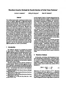
Figure 4: Electric guitar.
Figure 5: Finite element mesh.
Finite Element Methods The most general numerical techniques for solving PDEs are known as finite element methods (FEM). This section describes the structure of the equations that result upon application of FEM. Readers wishing a proper treatment of FEM should consult standard texts such as Becker, Carey, and Oden [2] for an introduction, and Strang and Fix [19] for mathematical analysis. Consider a heat conduction problem posed on the two-dimensional domain of Figure 4, an electric guitar. The problem is to find the steady state temperature u(x; y ) of the guitar, given that the guitar is exposed to specified heat sources. The physical behavior of this system is modeled by a partial differential equation1. We replace this continuous problem with a discrete approximation. Finite element methods achieve this goal by partitioning the domain into convex polygons or polyhedra, called finite elements. Elements are typically triangles or rectangles in two dimensions, and tetrahedra or rectangular blocks in three dimensions. The simplest element is the linear triangle, which possesses three nodes, one at each corner. A finite element mesh is a collection of elements (and nodes) covering a domain. Figure 5 shows a mesh of linear triangles covering the guitar. By considering the effects of the differential equation over each element, we construct an approximate system of linear equations of the form = (1)
Ku f
u
f
where = [u1 ; u2 ; : : : ; un]T denotes the temperatures at each of the n mesh nodes, the force vector denotes the heat sources at each mesh node, and the n � n stiffness matrix2 describes the interactions among the nodes due to the principle of conservation of energy, which governs heat conduction. Once we have solved for , we can interpolate between the nodal values to produce an approximate continuous solution u˜ (x; y ), which is piecewise linear on the mesh.
K
u
K
The structure of is illustrated in Figure 6, which shows a simple mesh composed of eight elements and nine nodes. Kij is nonzero only if nodes i and j share some common element. Hence, K24 is nonzero, K37 is zero, and Kii is nonzero for any i. For large meshes, is very sparse. The stiffness matrix is computed by summing the action of the differential equation over each individual element. Hence, K24 receives contributions from elements a and b, and K66 from elements f and g. The structure of is
K
�
�
The steady-state heat equation is ?r � k (x; y )ru(x; y ) = f (x; y ), subject to boundary conditions, where represents internal heat sources, and k (x; y ) is the thermal conductivity of the material. 1
2
The terminology for
K and f comes from structural mechanics, and has become widespread. 4
K f
f (x; y )
123456789 XXXX XXXXXX XXX XX XX XX X X XXXXXXX XX XXXX XXXXXX XXXXX X XXX
4 1 a e
b
c
d 7
5
2
3
6
9
h
g
f
1 2 3 4 5 6 7 8 9
K
8
4 1
a 2
3
b
5 7 6
8
9
G
c
d
g
h
e
E
Figure 6: A finite element mesh and its associated stiffness matrix adjacency graph E . X’s indicate nonzero matrix entries.
f
K, finite element graph
, and element
G
composed similarly; for example, f6 receives contributions from elements f and g. Given a finite element mesh, the associated finite element graph G is defined such that its vertices are the nodes of the mesh, and there is an edge between any two vertices that belong to a common element (see Figure 6). G is isomorphic to , in the sense that Kuv = 0 if (u; v ) 62 G. The associated element adjacency graph E is defined such that its vertices are the elements of the mesh, and there is an edge between any two vertices whose corresponding elements share a common node.
K
Solving the linear equation (1) accounts for most of the computation and interprocessor communication of solving the PDE. The linear system may be solved either by a direct method such as Gaussian elimination [11] or by an iterative method such as conjugate gradients [17]. In this article, we consider only iterative methods, which are much easier to parallelize than direct methods. Most iterative methods have as their central primitive the problem of computing the product of a large sparse matrix and a vector . For example, the iterative step of the conjugate gradient method consists of several vector operations and a single sparse matrix-vector multiplication. Note that over the course of a simulation the nonzero structure of the sparse matrix remains fixed (isomorphic to the finite element graph G), even though the values of the nonzero entries of may change over time (for instance, in nonlinear problems).
K
x
K
y Kx
K
involves the transfer of information along the edges of G, because the value The computation = of at node i depends on the values of at every node that is a neighbor of node i. Nodes do not interact directly with physically distant nodes; we will show how to take advantage of this locality to parallelize the computation.
y
x
5
Processor 1
Processor 2 4
4
1 a e
b
c 5
5
2
1 2 3 4 5 6
h
g
f 3
d 7
6
6
1 2 3 4 56 XXXX X X X X XX X X X XX XX XX X X X XX X X XX
8 4 5 6 7 8 9
K1
9
456789 XX X X XXXXX XXX X X X X X XX X XX XXXX XX
K2
Figure 7: Finite element mesh distributed among two processors. Each processor holds a subset of the elements and nodes; some nodes are mapped to more than one processor. Each processor maintains a processor stiffness matrix, which is a portion of the global stiffness matrix. X’s indicate nonzero matrix entries. Parallelizing Sparse Matrix-Vector Products
y Kx
To compute = on a set of processors, we must consider the data distribution by which vectors and matrices are stored. Although one might divide the set of nodes among the processors, it is more natural in finite element methods to partition elements. Each element of the mesh is assigned to a processor, and each mesh node resides on one or more processors, depending on which elements contain that node. The vectors and are stored in a distributed fashion according to this mapping. If a node i resides on several processors, the values xi and yi are replicated on those processors. The matrix is distributed so that Kij resides on any processor on which nodes i and j both reside. Figure 7 demonstrates this method of distributing data.
x
y
K
y Kx
is performed in two steps. First, each processor computes a local matrixThe multiplication = vector product over the subgraph of G that resides on that processor. Second, processors that share nodes communicate and combine their nodal y values into correct global values for each node. In Figure 7, Processors 1 and 2 must communicate to resolve the values of the shared nodes 4, 5, and 6. The data distribution is defined by embedding the element adjacency graph E into a graph H , which represents the underlying interconnection network of the target machine. (The vertices of H are the set of processors, and the edges of H are the set of communication wires connecting the processors.) For our purposes, an embedding of the graph E into a graph H consists of a many-to-one mapping from the vertices of E to the vertices of H , together with a mapping from each edge of E to a path (possibly of length zero) in H between the images of its endpoints. There are three primary measures of the efficiency of an embedding. One is its load, which is the 6
maximum number of finite element mesh edges mapped to any single processor. (To compute a sparse matrix-vector product, each processor does an amount of work roughly equal to the number of edges of G it is assigned.) The goal of keeping load low is to balance the parallel work among processors. The other two measures are the embedding’s dilation, which is the maximum path length between two processors that need to communicate (because they share nodes), and its congestion, which is the maximum number of edges of E whose corresponding paths travel through a single edge of H (the number of messages that cross the most congested communication wire). The goal of keeping dilation and congestion low is to minimize the total time required for communication. The relative importance of dilation and congestion for a particular machine will depend on its communication mechanism and method of routing. For instance, when store-and-forward routing is used, it is crucial to minimize the number of “hops” that a message takes, and the reduction of dilation is a primary concern. On the other hand, if the machine in question uses circuit-switched routing then the length of the routing paths is not as important as communication bottlenecks, so congestion becomes more important. It is not easy to find an efficient embedding of an element adjacency graph E to a graph H . To simplify the problem, it is traditionally broken into several steps. First, the mesh is partitioned — cut into subdomains, one per processor. An ideal partition will consist of subdomains having equal load, and will have small boundaries between subdomains (to minimize the communication between processors). We define the quotient graph E 0 derived from E and the partition. E 0 is a graph with a supervertex for each subdomain, and an edge between two supervertices if their corresponding subdomains must communicate (because they share mesh nodes). The second step is to place the quotient graph E 0 on the target machine H . This placement is a one-toone mapping of supervertices (and their corresponding subdomains) to processors. Finally, we route E 0 by finding a mapping of edges in E 0 to paths in H . It is not necessarily ideal to break the embedding problem into these steps. Better partitioning might be possible with knowledge of the topology of the target machine, and better placement might be possible if routing is considered simultaneously. However, finding an optimal embedding is difficult, and some simplifying assumptions are necessary. More importantly, we separate partitioning from placement and routing because partitioning can be done independently of any specific architecture, whereas placement and routing depend upon the topology and communication mechanisms of the target machine.
Archimedes At Carnegie Mellon we have built Archimedes, an automated system for solving partial differential equations over complex domains using distributed memory supercomputers. Archimedes is intended to allow researchers in engineering and science to solve real problems on unstructured meshes. Figure 8 diagrams the structure of Archimedes. A user provides two things: a description of the geometry of the problem domain, and an algorithm for performing finite element calculations that solve some physical problem. The problem geometry is the shape of the domain that will be modeled. In modeling earthquake ground 7
MVMUL(A,x) DOTPRODUCT (x,w,xw) SET(r=r/xw)
Problem Geometry
Finite Element Algorithm
Mesh Generator
Code Generator
Finite Element Mesh
Mesh Partitioner
Partitioned Mesh
Placement and Routing Multiprocessor
Figure 8: Structure of Archimedes. motion, this would be the shape of a valley and the surrounding rock. In flight vehicle aerodynamics, this would be the shape of the surface of the vehicle and surrounding air. Archimedes generates a mesh that fills the region of interest. Once a mesh is provided, Archimedes performs the partitioning, placement, and routing steps as necessary for a given architecture, using algorithms that will be described in the next few sections. Along with the problem geometry, the user writes a sequential algorithm for constructing and solving the finite element system for a specific problem. For instance, to solve our heat conduction problem, a user would write an algorithm to compute and , and solve for . The algorithm is written in a C-like syntax with built-in primitive operations tailored for finite element methods. This algorithm is machineindependent, and can be written without knowledge of the parallel machine’s underlying communication mechanisms. Archimedes compiles the algorithm into code for a specific machine.
K
f
u
8
Figure 9: Refinement of the original mesh. Mesh Generation High-quality unstructured meshes are difficult to generate, but not because it is difficult to generate an unstructured mesh. There are simple techniques for triangulating an arbitrary two-dimensional region, and although tetrahedralizing a three-dimensional region is much more complicated, there are straightforward techniques for doing so. A good survey of mesh triangulation methods in two and three dimensions is provided by Bern and Eppstein [3]. The real difficulty, though, is that a mesh generator should avoid producing elements with large aspect ratios — “skinny” triangles and tetrahedra, so to speak — because angles close to 180� cause a large discretization error [1], and very small angles cause the stiffness matrix to be ill-conditioned [6]. This constraint is difficult to reconcile with the correct meshing of arbitrary geometries.
K
Archimedes includes a two-dimensional mesh generator that triangulates complex geometries with high-quality elements, and furthermore allows the density of elements to vary and be controlled by the user, as was necessary to generate Figure 3. The meshing algorithm is due to Ruppert [16], who has proven that his algorithm generates meshes whose triangles have angles bounded between 20 � and 140� (except where there are input angles smaller than 20 � ; these cannot be improved). Archimedes currently has only rudimentary 3D mesh generation; work on an effective 3D mesher is in progress. The mesh generation algorithm serves another purpose. After the mesh is generated and the simulation completed, the approximate solution might not be as close to the exact solution as desired. A better solution can be found by refining the mesh and repeating the solution process. A mesh is refined by dividing some or all of its elements into a larger number of smaller elements, as in Figure 9. As the mesh is refined, the approximate solution converges to the exact solution u. Numerical analysts have developed a priori error estimates that show that the discretization error is reduced as the size of the largest edge is reduced. However, as we have explained, a constant element density is not always desirable. Hence, there are also a posteriori error estimates which estimate the discretization error on each element after the simulation, thereby providing a guide to refinement. Figure 9 was generated from Figure 5 as follows: Archimedes solved a heat conduction problem on the original mesh, and generated a posteriori error estimates on each element of the mesh. Based on the error estimates, it determined a maximum desired triangle area on each element. Archimedes’ mesh generator refined the existing mesh so that no triangle has area greater than the maximum allowed.
9
Figure 10: Partitioned guitar for sixty-four processor machine.
Figure 11: Sixty-four vertex quotient graph E 0 for partitioned guitar. Partitioning The two most common types of partitioning algorithm in the literature are known as recursive geometric bisection (RGB) and recursive spectral bisection (RSB). Both methods bisect a graph into two equal pieces, while attempting to minimize the size of the cut. Both methods are “recursive” because they first bisect a graph, then bisect each of the two resulting pieces, and so on; they therefore yield a number of subdomains that is a power of two. RSB [15] bisects a graph by exploiting spectral properties of its combinatorial structure. However, RSB does not take into account the positions of the graph’s vertices in space. While RSB usually produces excellent partitions in practice, it tends to be slow, as it relies on expensive eigenvector calculations. RGB uses the spatial coordinates of the vertices rather than the combinatorial structure of the graph, and typically executes more quickly. One of the main advantages of constructing Archimedes as a unified system is that the geometric information — the node coordinates and the node/element relationships — is readily available at all stages of the computation, including the partitioning and placement steps. Archimedes’ partitioner is an advanced recursive geometric bisection algorithm due to Miller, Teng, Thurston, and Vavasis [14], which finds provably good separators for a large class of geometrically defined graphs. A separator is a small set of edges whose removal divides the graph p into roughly equal pieces. For an n-vertex graph, it produces (with high probability) a separator of size O( n) in two dimensions, or 10
q
p Figure 12: Stereographic projection of a point onto a ball. Point p is mapped to point q . of size O(n2=3 ) in three dimensions. This is the best possible guarantee, in a worst-case asymptotic sense. In practice, our program usually generates better partitions than the theoretical worst-case bounds predict. Figure 10 illustrates our guitar partitioned into sixty-four pieces. Figure 11 illustrates the corresponding quotient graph E 0 . The Miller et al. algorithm runs in randomized linear time, and is made particularly efficient by a technique called geometric sampling. The idea is to choose a random sample of the vertices, then solve the partitioning problem over the sample. Thus the problem size is reduced, while the underlying geometric structure of the mesh ensures the quality of the result. Geometric sampling allows us to do most of the work on sets of only a few hundred vertices, even if the graph itself has millions of vertices. Another central idea of the algorithm is the stereographic projection of vertices from a graph to the surface of a ball. Figure 12 illustrates such a projection. Given a two-dimensional mesh in a plane, a three-dimensional ball is lain atop the plane. Each point in the plane is projected onto the ball by drawing a line that passes through the topmost point of the ball. Note that the projection is modified if the ball is resized or moved along the plane. Similarly, a three-dimensional mesh can be projected onto the surface of a four-dimensional ball. The algorithm uses the following steps, illustrated in Figure 13, to recursively bisect the element adjacency graph E : 1. Choose a random sample S of constant size from the vertices of E . 2. For a d-dimensional mesh, stereographically project S onto the surface of a (d + 1)-dimensional ball. Compute an approximate center point of the points projected on the surface of the ball. 3. Using the center point as a guide, modify the projection so that the center point coincides with the center of the ball. Intuitively, this is done by resizing or moving the ball relative to the graph E . 4. Choose a random d-dimensional hyperplane that passes through the center of the ball. The intersection of this hyperplane with the ball’s surface is a great circle. 5. Map this great circle back to the d-dimensional mesh to obtain a circle that partitions E into two pieces, E1 and E2 . If the circle intersects too many edges of E , go back to step 4 and choose another random hyperplane. 11
E 1
2 S
3
4
5
6
Figure 13: Illustration of partitioning algorithm. 1. A random sample S is chosen. 2. Points are projected to the surface of a ball. The large X indicates the center point of the projected points. 3. The projection is modified to move the center point to the center of the ball. 4. A random hyperplane splits the sample. The intersection of the plane and the surface of the ball form a great circle (bold). 5. The great circle is mapped to a circle in the plane. (Only a small section of the circle is shown here.) 6. Subdomains are bisected recursively. 6. Partition E1 and E2 recursively. Two aspects of the algorithm deserve deeper examination: center points and the random choice of hyperplanes. By definition, a center point for a set of n input points in d + 1 dimensions is a point c such that every -dimensional hyperplane through c has at most n � d=(d + 1) points on each side. A center point exists for any set of points, and can be found by linear programming. However, this method is much too slow to be practical; thus Archimedes uses a heuristic that finds good approximate center points in linear time. Clarkson et al. [8] show that the center point calculation is a good approximation for E even though it is based on the small random sample S . The sample size depends on the dimension but not the size of the input mesh. In theory, the subset size is proportional to d log d; in practice, we use several hundred points in two dimensions and about a thousand points in three dimensions. d
In theory, a randomly chosen hyperplane passing through the center of the ball has a 50% or better chance p of cutting only a small number of edges (O( n) in two dimensions, O(n2=3 ) in three). In practice, not 12
every hyperplane represents a good bisection. We therefore generate a number of hyperplanes, searching for one that gives a balanced partition with few edges cut. To improve our luck, the random hyperplanes are chosen from a biased distribution. Gremban [10] has suggested using the principal axis of the moment of inertia of the projected points to bias the random choice. A hyperplane perpendicular to the principal axis is likely to cross many fewer edges of E than a hyperplane parallel to the principal axis. Of course, the moment of inertia computation is fast because it is based only on the random sample S .
Placement and Routing The result of partitioning is the quotient graph E 0 , which describes the communication pattern among the processors during matrix-vector multiplication. E 0 should be embedded into the parallel architecture H such that the communication time is minimized. The notion of a good embedding thus depends on the target machine. We consider two communication models. With message passing, all routing decisions are made by the message passing system, and these decisions are hidden from the application. We also consider a connection-based model called the ConSet model. The set of interprocessor connections we need is broken up into a small number of phases, only one of which is active at a time. A phase consists of a subset of connections that can simultaneously be held active by the available hardware resources; the application controls which phase is instantiated at any given time. A connection can be used only if it belongs to the phase that is currently active. For a detailed discussion see Feldmann, Stricker, and Warfel [9]. The advantage of message passing is that no explicit routing need be done. The advantage of the ConSet model is that, because the structure of E 0 is known in advance, a communication compiler can choose routes and schedule communication so as to minimize network congestion. We discuss below two of our target machines, the iWarp and the Connection Machine CM-5, and how to embed E 0 into them. Our heuristics are inspired by algorithms from VLSI gate array layout [13].
Placement and Routing on the iWarp Our first target machine is the iWarp [5]. The iWarp is a distributed memory parallel computer whose processors are connected by a two-dimensional torus. The iWarp component is a VLSI chip that contains a processing agent and a communication agent. At the heart of the communication agent is a limited set of communication resources called queues. Queues on adjacent processors can be dynamically chained together to form pathways, which are point-to-point connections formed between processors using wormhole routing. Data traveling along a pathway passes from processor to processor automatically, with low latency, without disturbing the computations on intermediate processors. A pathway consumes a queue on each processor it touches. These ideas are illustrated in Figure 14. Because the number of queues per processor is limited, in general not all desired connections can be routed simultaneously. One way to address this problem is to use a simple message passing system: a pathway is dynamically set up directly between the source and destination, the data is transmitted, and 13
Figure 14: iWarp communication structures. Pathways are constructed by linking together queues. Processor 0 can send data to processor 2 without interfering with the computation on processor 1.
Figure 15: A succession of horizontal and vertical cuts defines the placement of the quotient graph on an 8 � 8 grid. the pathway is taken down to free up queues to be used for other messages. We have also implemented ConSet communication on the iWarp, which requires explicit routing but offers better performance. We shall address routing for ConSet in detail. The characteristics of the iWarp affect the efficiency of embeddings. Dilation is of minor importance because of the low latency of the pathways. Congestion is an important measure because all pathways sharing a communication bus are multiplexed over that link. In addition to these traditional measurements, we must address the constraint that a limited number of pathways can touch any particular processor at any particular point in time. This makes the vertex congestion of our embeddings, defined for each vertex in the target graph H as the total number of connections routed through (or into) that vertex, of paramount importance. For placement, as with partitioning, it is to our advantage to take into account the geometric information given in the original problem. We assign each node of E 0 a coordinate in two- or three-dimensional space by computing the center of mass of each subdomain (as illustrated in Figure 11). If our problem is threedimensional, we project E 0 to two dimensions to match our processor topology. One simple approach to placing a two-dimensional graph on the iWarp, or any two-dimensional mesh topology, is to simply halve the set of vertices repeatedly with alternating vertical and horizontal cuts (Figure 15), and map the vertices to the torus in the natural way. We further improve the placement with local hill-climbing search: we try swapping pairs of subdomains, and accept the swap if it reduces the sum of all connection lengths. processor 0
processor 1
processor 2
To route for the ConSet model, we must address two problems. First, each edge of E 0 must be assigned to one phase, during which its connection will be active. Second, each phase’s set of connections must be routed with a fixed number of queues per processor and with minimal congestion. We solve both problems together usingpathway sequential routing techniques based on weighted shortest path algorithms. queue
14
link processor 3
processor 4
processor 5
Phase 1
Phase 2
7
4
4
1
2
4
7
7
4
7
7
4
2
11
7
4
4
7
7
4
7
7
7
7
2
2
2
2
4
4
4
7
Figure 16: Connections are routed by finding the path of least cost from among the communication phases. The cost of each processor is shown; the cost of a processor increases nonlinearly with the number of connections through that processor. Our sequential routing algorithm begins by sorting all connections, from longest to shortest, by distance (in H ) from source to destination. Each vertex of H (in each phase) is assigned an initial cost of one. We define the cost of a path between two vertices in H to be the sum of the cost of the vertices along the path. Connections are routed one by one, each along a shortest path from all possible phases (Figure 16). Each time a connection is successfully routed, the cost of each vertex along the path is increased. (The increase is nonlinear, and the cost of a vertex whose queues are all used is infinite.) If all connections can be routed this way, we have found a solution, but not necessarily a good one, because the quality depends on the order in which connections are routed. Whether or not all connections are successfully routed, the communication compiler tries to improve the routing with a “ripup and reroute” stage, wherein routes are repeatedly selected to be ripped up, and the vertex costs are updated; then the connections are rerouted, often along less congested routes. During this stage it is often possible to find a route for a previously unroutable connection. The question remains, how do we know how many communication phases are required? The routing algorithm is fast enough that we simply begin by trying to route with one phase; if routing is not successful, the number of phases is increased until the algorithm succeeds. When routing is complete, a schedule is generated that describes a good order in which to exchange messages during each phase. The placement, routing, and scheduling heuristics are all described in detail by Feldmann et al. [9]. Figure 17 illustrates the quotient graph of Figure 11, placed and routed on a 64-processor iWarp by our algorithms. We have tried other heuristics for placement and routing, including simulated annealing and linear programming, but they have not performed as well.
Placement on the Connection Machine CM-5 Another target machine is the Connection Machine CM-5 [20]. The CM-5 is a distributed memory parallel computer whose computational nodes are connected by a fat-tree network [12]. The network supports message passing communication, as well as efficient primitives for synchronization, broadcast, and scan. 15
9
9
8
8
7
7
6
6
5
5
4
4
3
3
2
2
1
1
0 0
2
4
6
0 0
8
2
4
Figure 17: Interprocessor connections on a 64-processor iWarp for the quotient graph cation phases are required.
6 E
8
0
. Two communi-
The network topology, a fat-tree, is best suited for communication patterns with hierarchical locality. The network is organized such that groups of 4 processors have the highest bandwidth among themselves, groups of 16 processors have a slightly lower bandwidth, and anything past a 16 processor boundary has yet a lower bandwidth. This hierarchical locality of a fat-tree is well suited for recursive bisection partitioners, as the separators give a hierarchical decomposition. While partitioning E , we derive a binary cut tree T , which is the recursion tree of the partitioning algorithm. The leaves of T represent the subdomains (vertices of E 0 ). We can collapse alternate levels of T to obtain a 4-ary tree whose structure matches that of the fat-tree network, and embed this tree into the fat-tree in the natural way. Because the network hardware takes care of routing, we do not need to specify an embedding of the edges.
Code Generation Archimedes program are written in C, augmented with high-level operations specific to finite element methods. Archimedes’ output is also C code, with FEM libraries and machine-specific communication code added. There are several reasons why parallel applications should be automatically generated from an augmented language. First, few scientists or engineers want to invest the time necessary to learn how to program a multicomputer. Second, Archimedes’ high-level commands allow one to quickly change code and experiment with different linear solvers, preconditioners, ODE integrators, and so on. Third, a general-purpose finite element code generator ensures that the effort spent writing optimized parallel linear solvers and other application code can be easily reused for different simulations. Fourth, every application written in the language can be ported to new architectures by porting the code generator. We illustrate Archimedes’ language with an excerpt from code written to solve the heat equation. In addition to the usual C data types, Archimedes has several distributed data types, including vectors 16
Ku f
and sparse matrices. Consider the inner loop of a simplified conjugate gradient code [17] to solve = . Below, the MATRIX keyword declares a distributed sparse matrix, and the NODEVECTOR keyword declares distributed vectors.
K
MATRIX ; NODEVECTOR ; ; ; ; float dq, norm, firstnorm, oldnorm, alpha, beta;
udqr
(Setup code is omitted here.) while (norm > EPSILON � firstnorm) f beta = norm / oldnorm; = + beta � ; MVPRODUCT( ; ; ); DOTPRODUCT( ; ; dq); alpha = norm / dq; = + alpha � ; = - alpha � ; oldnorm = norm; DOTPRODUCT( ; ; norm);
d r
u u r r
d Kdq dq d q rr
g
Several lines of code above perform mixed scalar/vector arithmetic; these lines can be executed without any communication. The MVPRODUCT operation forms the product = , and the DOTPRODUCT operation forms the products dq = � and norm = � , each requiring communication. Because many simulations can be implemented with only these two communication primitives, a simple version of Archimedes is easy to port to new architectures. Although Archimedes includes a variety of other commands that implement stiffness matrix formation, preconditioning, and other operations, these do not require communication and are trivially portable.
d q
r r
q Kd
In addition to ordinary iterative methods like conjugate gradients, Archimedes includes support for a numerical technique known as domain decomposition, which can greatly improve the solution time for time-dependent simulations. Domain decomposition methods combine direct methods for solving linear systems with iterative methods, in such a way that they are easy to parallelize (recall that pure direct methods are not). Briefly, each processor uses standard Gaussian elimination to eliminate the interior nodes of its subdomain; then an iterative method is used to solve the linear system for the shared nodes on the boundaries of subdomains. Further details are given in the survey by Chan [7] and the article by Shewchuk and Ghattas [18].
Experience and Conclusions The events that led to the development of Archimedes are informative. In late 1991, civil engineers at Carnegie Mellon began exploring the use of parallel computers for modeling earthquake-induced ground motion. They manually implemented a simulation on the Thinking Machines CM-2. To obtain fast enough 17
communication for the simulation to be useful, they had to use a block-structured mesh and painstakingly partition it by hand. Unfortunately, because the gradation of the block-structured mesh was insufficiently flexible, the mesh used smaller elements than were desired in the rock surrounding the valley. These smaller elements made necessary the use of small time steps to ensure stability of the numerical method, and so the solver was forced to take many more iterations than the physics required. Switching to a method that does not exhibit these advantages was considered, but would have entailed a complete rewrite of the code. Parallel computers, rather than a tool, were becoming an impediment to doing science! Frustrated by the painstaking level of detail required to create efficient programs, the engineers sought out computer scientists at Carnegie Mellon for assistance. During these discussions, we realized that by exploiting exploiting prior work in mesh generation and VLSI routing, and our own ongoing work in graph partitioning and parallelizing compilers, it would be possible to fully automate the irregular finite element modeling process. The Archimedes collaboration was born. Since its original implementation for the iWarp and CM-5 systems, we have retargeted Archimedes to the Intel Paragon, as well as individual workstations to ease the debugging process. Other architectures are planned. It generally requires a week or two of effort to retarget the code generator. Archimedes has duplicated the original 3D seismic ground motion study, and is currently being used on a production basis to model ground motion in 2D and 3D basins [4]. Ultimately, Archimedes will be used to model the entire Los Angeles basin.
References [1] BABUSˇ KA, I., AND AZIZ, A. K. On the Angle Condition in the Finite Element Method. SIAM Journal on Numerical Analysis 13, 2 (Apr. 1976), 214–226. [2] BECKER, E. B., CAREY, G. F., AND ODEN, J. T. Finite Elements: An Introduction. Prentice-Hall, Englewood Cliffs, New Jersey, 1981. [3] BERN, M., AND EPPSTEIN, D. Mesh Generation and Optimal Triangulation. In Computing in Euclidean Geometry, D.-Z. Du and F. Hwang, Eds., vol. 1 of Lecture Notes Series on Computing. World Scientific, Singapore, 1992, pp. 23–90. [4] BIELAK, J., KALLIVOKAS, L. F., XU, J., AND MONOPOLI, R. Finite Element Absorbing Boundary for the Wave Equation in a Halfplane with an Application to Engineering Seismology. In Third INRIA-SIAM Wave Propogation Conference (Juan-les-Pins, France, Apr. 1995). [5] BORKAR, S., COHN, R., COX, G., GLEASON, S., GROSS, T., KUNG, H. T., LAM, M., MOORE, B., PETERSON, C., PIEPER, J., RANKIN, L., TSENG, P., SUTTON, J., URBANSKI, J., AND WEBB, J. iWarp: An Integrated Solution to High-Speed Parallel Computing. In Supercomputing ’88 (Kissimmee, Florida, Nov. 1988). [6] CAREY, G. F., AND ODEN, J. T. Finite Elements: A Second Course. Prentice-Hall, Englewood Cliffs, New Jersey, 1983. [7] CHAN, T. F., AND MATHEW, T. P. Domain Decomposition Algorithms. In Acta Numerica 1994. Cambridge University Press, New York, 1994, pp. 61–143. 18
[8] CLARKSON, K. L., EPPSTEIN, D., MILLER, G. L., STURTIVANT, C., AND TENG, S.-H. Approximating Center Points with Iterated Radon Points. In Proceedings of the Ninth Annual Symposium on Computational Geometry (San Diego, California, May 1993), Association for Computing Machinery, pp. 91–98. [9] FELDMANN, A., STRICKER, T. M., AND WARFEL, T. E. Supporting Sets of Arbitrary Connections on iWarp through Communication Context Switches. In Fifth Annual ACM Symposium on Parallel Algorithms and Architectures (Velen, Germany, July 1993), Association for Computing Machinery, pp. 203–212. [10] GREMBAN, K. D., MILLER, G. L., AND TENG, S.-H. Moments of Inertia and Graph Separators. In Proceedings of the Fifth Annual ACM-SIAM Symposium on Discrete Algorithms (Arlington, Virginia, Jan. 1994), Association for Computing Machinery, pp. 452–461. [11] HEATH, M. T., NG, E., AND PEYTON, B. W. Parallel Algorithms for Sparse Linear Systems. SIAM Review 33, 3 (Sept. 1991), 420–460. [12] LEISERSON, C. E., ABUHAMDEH, Z. S., DOUGLAS, D. C., FEYNMAN, C. R., GANMUKHI, M. N., HILL, J. V., HILLIS, W. D., KUSZMAUL, B. C., ST. PIERRE, M. A., WELLS, D. S., WONG, M. C., YANG, S.-W., AND ZAK, R. The Network Architecture of the Connection Machine CM-5. In Proceedings of the Fourth Annual ACM Symposium on Parallel Algorithms and Architectures (San Diego, California, June 1992), Association for Computing Machinery. [13] LENGAUER, T. Combinatorial Algorithms for Circuit Layout. Applicable Theory in Computer Science. John Wiley & Sons, Chichester, England, 1990. [14] MILLER, G. L., TENG, S.-H., THURSTON, W., AND VAVASIS, S. A. Automatic Mesh Partitioning. In Graph Theory and Sparse Matrix Computation, A. George, J. R. Gilbert, and J. W. H. Liu, Eds. Springer-Verlag, New York, 1993. [15] POTHEN, A., SIMON, H. D., AND LIOU, K.-P. Partitioning Sparse Matrices with Eigenvectors of Graphs. SIAM Journal on Matrix Analysis and Applications 11, 3 (July 1990), 430–452. [16] RUPPERT, J. A New and Simple Algorithm for Quality 2-Dimensional Mesh Generation. Tech. Rep. UCB/CSD 92/694, University of California at Berkeley, Berkeley, California, 1992. To appear in Journal of Algorithms. [17] SHEWCHUK, J. R. An Introduction to the Conjugate Gradient Method Without the Agonizing Pain. Available by anonymous FTP to WARP.CS.CMU.EDU (128.2.209.103) as quake-papers/painlessconjugate-gradient.ps, Aug. 1994. [18] SHEWCHUK, J. R., AND GHATTAS, O. A Compiler for Parallel Finite Element Methods with DomainDecomposed Unstructured Meshes. In Proceedings of the Seventh International Conference on Domain Decomposition Methods in Scientific and Engineering Computing (1994), D. E. Keyes and J. Xu, Eds., vol. 180 of Contemporary Mathematics, American Mathematical Society, pp. 445–450. [19] STRANG, G., AND FIX, G. J. An Analysis of the Finite Element Method. Prentice-Hall Series in Automatic Computation. Prentice-Hall, Englewood Cliffs, New Jersey, 1973. [20] THINKING MACHINES CORPORATION. The Connection Machine CM-5 Technical Summary. 1991. 19