Topical Editor: Prof. Christian Wöhler, 3D RESEARCH 03, 06 (2010) 10.1007/3DRes.03(2010)06
3DR EXPRESS
w
Automatic Scan Registration Using 3D Linear and Planar Features Jian Yao • Mauro R. Ruggeri • Pierluigi Taddei • Vítor Sequeira
Received: 25 August 2010 / Revised: 15 September 2010 / Accepted: 12 October 2010 © 3D Research Center and Springer 2010
Abstract * We present a common framework for accurate and automatic registration of two geometrically complex 3D range scans by using linear or planar features. The linear features of a range scan are extracted with an efficient splitand-merge line-fitting algorithm, which refines 2D edges extracted from the associated reflectance image considering the corresponding 3D depth information. The planar features are extracted employing a robust planar segmentation method, which partitions a range image into a set of planar patches. We propose an efficient probabilitybased RANSAC algorithm to automatically register two overlapping range scans. Our algorithm searches for matching pairs of linear (planar) features in the two range scans leading to good alignments. Line orientation (plane normal) angles and line (plane) distances formed by pairs of linear (planar) features are invariant with respect to the rigid transformation and are utilized to find candidate matches. To efficiently seek for candidate pairs and groups of matched features we build a fast search codebook. Given two sets of matched features, the rigid transformation between two scans is computed by using iterative linear optimization algorithms. The efficiency and accuracy of our registration algorithm were evaluated on several challenging range data sets. Keywords: 3D Scan Registration, Feature Extraction and Matching, Planar Segmentation, 3D Edge Extraction, Congruent Set Search, Feature Range-Query.
1. Introduction In the past decade, there was a growing interest for 3D reconstruction and realistic 3D modelling of large-scale scenes such as urban structures. Applications of such Jian Yao1( ) • Mauro R. Ruggeri1 • Pierluigi Taddei1 • Vítor Sequeira1 1 Institute for the Protection and Security of the Citizen (IPSC) European Commission - Joint Research Centre (JRC) e-mail:
[email protected]
models include virtual reality, telepresence, digital factory, digital cinematography, digital archaeology, urban planning, inspection and reverse engineering, and other areas. Commonly these applications require a combination of range sensing technology with traditional digital photography. Those applications that employ only digital images extract 3D information using either a single moving camera or a multi-camera system, such as a stereo rig. In both cases the system extracts and matches distinctive features (typically key points) across all the available images and estimates their 3D positions and the camera parameters14, 34, 35. It is then possible to exploit the result of this first step to perform a dense point reconstruction by estimating a depth map for each image26, 34, 38. On the one hand these approaches are useful for those applications requiring a robust and low cost acquisition system. On the other hand, range sensing technology yields much higher precision and resolution. Moreover each single range acquisition can cover a full 360o × 180o panoramic view and requires only few minutes. Thus, the range sensing technology represents an effective and powerful tool for achieving accurate geometric representations of complex surfaces of real-world scenes at different scales with different accuracy levels13, 15, 29. In recent years a lot of new commercial 3D laser scanners are able to provide satisfied measurement accuracy for different applications. 3D laser scanners are able to be used to capture a complex real scene through multiple range scans acquired from different positions to fully represent the scene reducing the number of occluded surfaces. A range scan represents a partial region of the scene through a range image, i.e., a cylindrical or spherical image containing depth information for each pixel. It can also be accompanied by a reflectance image and a colour image storing for each pixel the portion of light reflected from the corresponding surface point and its colour, respectively. The reflectance image corresponding to a panoramic range image of an indoor scene is displayed in Fig. 2. From a range image it is then possible to obtain the corresponding point cloud in 3D space whose coordinate system is centred at the scan sensor central point. Thus, we
2
need a systematic and automatic way to align, or register, multiple 3D range scans to represent and visualize them in a common coordinate system. Geometrically, given a range scan S considered as reference, the problem of registration consists of finding the rigid transformation T , which optimally aligns another scan S ′ with S in its coordinate system. The Iterative Closest Point (ICP) algorithm3 is the de facto standard to compute T . It is basically an optimization method that starts from an initial estimate of T and iteratively refines it by generating two sets of corresponding points on the scans and minimizing an error metric, e.g., the sum of squared distances between corresponding points. Although several variants of ICP were proposed28 to improve its efficiency, the main problem is to achieve a good initial estimate of T since the ICP optimization can easily stop in local minima. The problem of automatically aligning two range scans was solved with a wide variety of approaches24. Most of these approaches extract two sets of feature points, which are automatically matched to recover a good approximation of T . Aiger et al.1 proposed to automatically match congruent sets of four roughly coplanar points to solve the Largest Common Point set problem. Congruent sets of points have similar shapes defined in terms of point distances in Euclidean 3D space and surface normal deviations. The best match between congruent sets is randomly found by utilizing the RANdom SAmple Consensus (RANSAC) approach10. Some researchers proposed to utilize shape descriptors to identify sets of candidate feature points to be matched. Gendalf et al.12 used a 3D integral invariant shape descriptor to detect feature points, which are matched in sets of three items using a branch-and-bound algorithm. Other interesting shape descriptors invariant with respect to the rigid transformation are used to identify feature points such as, scale invariant feature transforms (SIFT)s20, 22, 36 or Harris corners20 extracted from reflectance images36, 3D SIFT-like descriptors extracted from triangle meshes approximating the point clouds37, spin images16, 17, and extended Gaussian image23. Other approaches automatically recover the rigid transformation between two range scans by extracting and matching two sets of higher-level features, e.g., planes6, 8, 30 , lines30, circles5, spheres11 and other fitted geometric primitives27. Dold and Brenner8 presented an automatic registration of terrestrial scan data achieved through matching pairs of planar patches extracted from the scans. Geometrical and laser scanning attributes associated to the planar patches are used to exclude implausible correspondences during matching. Stamos et al.6, 30 proposed to utilize the fitted planes in the surface and intersecting lines on those planes to match two scans. The extracted lines mostly correspond to real surface edges (surface normal and/or depth discontinuities) in 3D space. Their proposed approaches provide accurate registration results in scenes of urban nature with plenty of planes, but will fail in scenes that do not contain a sufficient amount of lines, depending on the extracted planes. Chen and Stamos5 proposed to match circular features extracted from range images. However, circular features only exist in some specific scenes. Franaszek et al.11 developed an automatic
3D Res. 03, 06 (2010)
range scan registration method by detecting spheres locally fitted to the point cloud, which are aligned by finding three pairs of matching spheres’ centres. Rabbani and van den Heuvel27 proposed to first extract geometric primitives like planes, cylinders and spheres, which are then matched automatically using their geometric information. The matching was performed through a constrained search method based on several steps of pruning a search tree using geometrical constraints. 1.1. Overview and Contributions We present a new method that utilizes geometric features to achieve automatic registration. Our algorithm is summarised in Fig. 1. It automatically aligns two range scans S and S ′ by finding two congruent sets of their features leading to a good estimate of the transformation T between the corresponding point clouds. T is then further refined via the ICP algorithm.
Fig. 1: The flowchart of our registration algorithm.
In particular our algorithm employs 3D linear features or planar features. 3D line segments are directly detected from edge contours extracted from 2D reflectance images instead of getting the plane-plane intersecting lines as in6, 30 . Thus the considered lines origin not only from real surface edges but also from intensity edges (no obvious surface normal and depth discontinuities). Planar features are extracted by firstly partitioning the range image into a set of rectangle blocks of size 2 N × 2 N and fitting a planar patch to all points of each block. Blocks that are not successfully fitted as planar patches, are iteratively partitioned into sub-blocks of size 2( N − k ) × 2( N − k ) until reaching a minimum size of 4× 4 . Secondly, we iteratively merge planar patches and discard unclassified rectangle blocks or points. Finally the boundaries between planar patches are refined by relabelling.
3D Res. 03, 06 (2010)
3
Once we extract features from two range scans S and S ′ , our algorithm randomly searches for two sets of congruent groups of features in S and S ′ which lead to the best estimate of T . This is achieved by following the RANSAC approach10, which mainly consists of a main iteration loop, in which possibly matched candidates are randomly selected and verified until a good solution to the problem is found or the number of iterations exceeds a predefined threshold I max . The search of possibly matched features forming congruent groups in S and S ′ is performed as range-query on a codebook computed from the features of S ′ . The main loop of our RANSAC-based algorithm comprises the following steps:
2) Utilizing resolution sensitive weight functions to robustly recover the rigid transformation between congruent groups of features with different resolutions, as presented in Sections 2.2.1 and 3.2.1.
1) Random selection of a set of M features in scan S . 2) Congruent group selection of M similar (or possibly matched) features in scan S ′ . This is achieved by using a codebook to efficiently find similar features and an algorithm to isolate congruent groups of size M , as described in Sections 2.2.2 and 3.2.2. ~ 3) Estimation of the transformation T between S and S ′ . In Section 2.2.1 we describe a new method to ~ estimate T based on corresponding 3D line segments, which extends the algorithm presented in19 by introducing a novel weight function, which is capable of robustly handling features with different resolutions. In Section 3.2.1, a point-to-point error metric between corresponding planar features with parametric plane representations is iteratively minimized to achieve the ~ best estimate of T . 4) Verification and refinement of the transformation. ~ T is verified on all matched features and is further refined as explained in Sections 2.2.1 and 3.2.1 if it is considered as a good estimate. ~ 5) Updating best transformation T if Quality(T) > Quality(T) as defined in Eq. (13) for linear features and Eq. (29) for planar features.
2. Registration Using Linear Features
In Section 2.2.3 we present a variant of this RANSACbased algorithm, which we call the probability-based RANSAC approach, that improves the random selection step by employing a weight function approximating the probability of each pair of features in scan S to be matched with one in scan S ′ . As summarised in Fig. 1 these probabilities are computed before the random selection and updated at each successful RANSAC ~ iteration after refining T . This approach allows reducing the number of evaluations required by the RANSAC to detect a correct set of matched features. This is crucial, in particular, when the two scans have a small overlap region, and thus when the percentage of matched features is low. As in27, our method is able to match different types of geometric primitives. However, our algorithm is also robust with respect to different sampling densities. This is achieved by using the two following novel approaches: 1) Employing suitable techniques to adaptively compute thresholds to robustly match pairs of linear and planar features. These techniques presented in Sections 2.2.2 and 3.2.2 allow to efficiently match congruent groups of similar features with different resolutions by using suitable codebooks to perform adaptive range-queries.
Our matching algorithm can be applied to any other types of features, by only providing a proximity function and a constrain criterion for the features considered. In Section 4, the robustness and the efficiency of our proposed registration methods were statistically tested on several challenging range data sets acquired from indoor and outdoor scenes.
Our proposed automatic registration between two scans using linear features is described in this section. Initially we extract a set of linear features from the reflectance image of each range image using an edge detection method. Then two scans are automatically aligned by recovering the rigid transformation from their associated linear features sets. 2.1. 3D Linear Feature Extraction
Fig. 2: Reflectance image (top) and edge map (bottom).
In this section we describe a simple method to extract a set of 3D linear features from a range image based on edges extracted from its corresponding 2D reflectance image. An extracted 2D edge falls in one of the following three types: (a) edge caused by surface normal discontinuities (crease edge), (b) edge caused by depth discontinuities (step edge), and (c) edge caused solely by intensity discontinuities (intensity edge). Most of 3D edge detectors6 are able to find only edges of the first two types. However, most of these edges can also produce relevant intensity changes on 2D reflectance images, which result in intensity edges. Thus, in order to detect more edge contours for further 3D linear feature extraction, we utilize the edge detection with segment-based hysteresis thresholding proposed by Wang et al.32. This detector is applied directly to the reflectance
4
3D Res. 03, 06 (2010)
image and extracts 2D edges which we then associate to 3D points using the range image. Moreover, this method introduced a novel saliency measure called supporting range, which measures, for each edge pixel, the range along the gradient direction in which its gradient magnitude is a local maximum. Finally, unlike the Canny detector4, the proposed hysteresis thresholding approach is based on segments (continuous edge contours) instead of individual pixels. Experiments conducted on a lot of reflectance images show that it can robustly detect most edge pixels on object boundaries even if they have very low gradient magnitude. A typical example is shown in Fig. 2. By considering 2D edge points extracted from a reflectance image, we detect linear features by the following three steps. 1) Identifying meaningful edge points. We collect a set of continuous 2D edge contours with enough edge points and remove the invalid ones by considering their 3D information. An edge contour consisting of N edge points is defined as C = {x i|x i ∈ ℜ 3 }iN=1 . In some cases step edges are not caused by real 3D surface boundaries but by one surface occluding another (occlusion edges). Occlusion edges are usually noisy and either associated to foreground or background points. Foreground points lie on the real surface boundaries and are considered to be meaningful for linear features, while background points lie on the fake boundaries of the occluded surfaces, having unlikely matches in other scans acquired from different viewpoints. Consider an edge point p and let b1 and b 2 be its two neighbouring points perpendicular to the gradient orientation in p . We say that p is an occlusion edge point and b1 is a foreground point on a surface boundary in ℜ3 if: || p − b1 ||> rd || p − b 2 ||, depth (p) > depth (b1 ),
(1)
where || ⋅ || denotes the L2-norm, depth (x ) denotes the depth value of the point x from the scan sensor centre, and rd is a constant ( rd = 10 was used in this paper). The 3D coordinates of occlusion edge points are replaced by those of their corresponding foreground points. 2) Filtering noisy edge points. For each point x of the edge contours we calculate a median adjacent distance ~ d c (x) . This value is defined as the median of distances || xi −1 − xi || between two adjacent 3D points on the contour close to x . In particular we consider a median window of ~ 10 elements centred at point x , i.e., d c (x i ) = median ij+=5i − 5 || x j −1 − x j || . A point xi ∈ C will be considered as a noisy point and eliminated from the contour C if its distance to the closest neighbourhood edge point is too high with respect to the calculated median adjacent distance in xi , which is expressed in a mathematical form as: ~ min(|| xi −1 − xi ||, || xi − xi +1 ||) > α c d c (xi ), (2)
where α c is a constant ( α c = 5 in this paper).
3) Fitting 2D contours to 3D line segments. We fit the edge points of a 2D contour to a set of 3D line segments by utilizing the popular standard split-and-merge algorithm25 with small modifications. Initially, we create a line segment in ℜ3 by connecting two endpoints of the whole contour segment and compute the distances of the points on the contour segment to the line. The contour segment is regarded as a successfully extracted line segment if the maximal point-to-line distance at the point p is less than a ~ threshold tm = α m d fc and most (90% in this paper) of point~ to-line distances ~ are less than a threshold t p = α p d fc where α m > α p and d fc is the median adjacent distance of the currently processed contour segment. These points are called as the line inlier ones. Otherwise, we split the contour segment at the maximal deviation point p into two segments if its length is greater than a threshold. In this way, the algorithm recursively splits the contour until all split segments have been checked. The inlier points of the successfully split contour segments are fitted to 3D lines using least squares. Those line segments with a small gap which are collinear are then merged into a single one. After applying the split-andmerge algorithm on all the edge contours, we further merge collinear line segments into new line segments by keeping those merged, since they are useful for line matching as shown in Section 2.2. A linear feature corresponding to an extracted 3D line ~ segment is represented as a 5-tuple l = (Ψ, x s , xe , v, d ) where: • Ψ is a set of 3D inlier points belonging to the line segment (which, in general, may not lie on the line segment), • x s ∈ ℜ3 and x e ∈ ℜ3 are the two endpoints of the line segment generated by projecting all inlier points in Ψ on the line segment, • v ∈ ℜ3 is the orientation of the line segment (i.e., v = (xe-x s ) || xe-x s || ), and ~ • d is the median of median adjacent distances of all the inlier points in Ψ .
2.2. Linear Feature Matching In this section we describe our automatic registration algorithm to align two overlapping range scans S and S ′ taken from different viewpoints using linear features. The aim is to recover the transformation T = (R, t) from the scan S to the scan S ′ , where R is the 3 × 3 rotation matrix and t = [t x , t y , t z ]T is the translation vector. The main structure of our algorithm is explained in Section 1.1 and summarised in Fig. 1. The details of our two variants of the RANSAC based algorithm for linear features matching are described in Section 2.2.3. The estimation of the transformation as well as its refinement are presented in Section 2.2.1. In Section 2.2.2 we describe the congruent group selection of M similar linear features through a codebook-based fast matching algorithm. 2.2.1. Transformation Estimation
3D Res. 03, 06 (2010)
5
Let L = {l i }iL=1 and L ′ = {l′m}mL′=1 be two sets of 3D linear features extracted from S and S ′ , respectively. Generally, the problem of recovering the transformation between S and S ′ can be solved if two or more pairs of matched nonparallel linear features are found between L and L ′ . By using M ( M ≥ 2) pairs of matched non-parallel linear features, the method proposed in39 provides a closed-form solution for the transformation T . It exploits only the orientations (directions) and positions of the lines to estimate the transformation, avoiding to use the endpoints of the extracted line segments which can never be exactly localized. The extracted 3D linear features are not very accurate due to noise on 2D edges and 3D data. In addition, scanned data usually have different point densities, which are related to the distances and the incident angles of the scanned surfaces with respect to the scanner sensor position and orientation, respectively. Normally, short distances and small incident angles lead to surfaces with high point densities and accuracies, which we consider as high resolution regions. The overlapping region of two scans often presents different resolutions, which may lead to mismatches of linear features. Our method to match linear features is inspired by19 and uses a novel weighting technique to robustly recover the rigid transformation of two sets of M matched linear features. Linear features are matched considering line distances together with orientations to improve the matching effectiveness of line segments with different resolutions. M pairs of matched non-parallel linear features are used to compute the transformation T between two range scans. T is verified by transforming all linear features in L and checking whether they have matches in L ′ . Once verified, T is globally refined by using all matched linear features between L and L ′ . However, the closed-form solution used in19 to compute T is not robust when the overlapping regions (i.e., matched linear features) between two scans present different resolutions. In this context, it is difficult to select M pairs of matched linear features to accurately estimate the initial transformation and then refine it after verification. Given K linear features in L having matches in L ′ , the probability of successfully selecting M linear features in L (whose cardinality is L ) with matches in L ′ is p( M ) ≈ ( K L) M . Increasing the accuracy of the initial transformation estimate by increasing M is not a good strategy for random selection because p( M ) quickly decreases. Indeed, when K L is small and M is large, p ( M ) is very low. To recover a good initial transformation using a small number of M pairs of matched linear features, we follow the robust line matching approach presented in19 by introducing a novel weight function, which is capable of robustly handling linear features with different resolutions. Our method iteratively minimizes the following distance measure:
D (L ′M , TL M ) =
∑
w( l ′n , T0 l n ) D p (l ′n , Tl n ),
(3)
l n ∈L M , l ′n ∈L ′M
where we assume that L M = {l n }nN=m1 ∈ L matches L ′M = {l′n}nN=m1 ∈ L ′ and the pairwise distance measure between linear features l′n and Tl n is given by:
D p (l ′n , Tl n ) = ∑|l n|⋅ || (x& ′n + sn v′n ) − Rxn − t ||2 +|l n|3 (1 − vTn Rv′n ) / 6, if |l n| ≤ |l′n|, x ∈Ψ (4) 2 3 T ∑|l′n|⋅ || x′n − R(x& n + sn vn ) − t || +|l′n| (1 − vn Rv′n ) / 6, if |l n| > |l′n|, x′ ∈Ψ′ k
nk
n
nk
n
k
k
k
where x& is the line middle point (i.e., x& = (x s + xe ) 2 ), |l| denotes the line length (i.e., |l| =|| x s − xe || ), and snk is the shift parameter of a point on the line l n with respect to x& . The transformation T operating on L M is given by Tx& n = Rx& n + t, Tv n = Rv n .
(5)
The weight w(l′n , T0 l n ) is defined as: |l′n ∩ T0 l n| |Ψ |d~′2 , if |l n| ≤ |l′n|, w(l′n , T0 l n ) = n n |l ′ ∩ T l | n ~02 n , if |l n| > |l′n|, |Ψn′|d n
(6)
where the transformation T0 is recovered by the closedform solution or in the last linear iteration and l a ∩ l b denotes the overlapping line segment of two linear features l a and l b . Since, in general, the transformed Tl and l ′ are not accurately collinear, we produce the overlapping line segment by projecting the two endpoints of one line segment to another line segment. The introduced weight function w considers the density and the sampling distribution of the overlapping line segment of two linear features to weight their distance Dp . This approach relevantly reduces the impact of different resolutions in the matched linear features on the estimation accuracy of T . At each iteration our algorithm computes the transformation T and updates the shift parameters {snk } until the rotation and translation differences between two consecutive iterations are less than certain thresholds. 2.2.2. Codebook-Based Fast Matching of Congruent Groups of Linear Features Given a group of M randomly selected linear features in L , we aim at finding a congruent group of linear features among all possible O(L′ M ) groups of L′ to recover the transformation T . Two groups of linear features are considered to be congruent if they are approximatively similar in shape and have the same distribution in the 3D space. Searching congruent sets of M linear features with a blind hypothesis-and-test approach would require to test O(LM L′ M ) groups of linear features, which is impractical due to the size of the search space. In this section we present a method to solve this problem by reducing the search space and the search time of similar groups of linear features. In the following we present: (a) a geometrical constraint to match pairs of linear features; (b) a codebook to efficiently search similar pairs of linear features; (c) an algorithm to efficiently find congruent groups of M linear features in L and L′ . Geometrical constraint to match pairs of linear features. To check whether two groups of linear features are congruent or not we need a method to robustly compare
6
3D Res. 03, 06 (2010)
their pairs of linear features. Two linear features l i and l j in L are compared through computing the line orientation angle odif (l i , l j ) = acos( v iT v j ) and the line shortest distance defined as d (l i , l j ) = min∀x∈li ,∀y∈l j || x − y || . Note that d (l i , l j ) considers l i and l j as infinite lines instead of line segments. These two measures are invariant with respect to the rigid transformation of L . For a pair of nearparallel linear features (li , l j ) assuming |l i| > |l j| , we set d (l i , l j ) = d (l i , x& j ), x& j ∈ Ψ j , i.e., the distance of the midpoint x& j of l j to the line of l i . In addition, since the line orientation (direction) is arbitrary, the orientation angle between two linear features is converted into the range [0, π 2] , i.e., odif (l i , l j ) = min(π − acos( v iT v j ), acos( viT v j )) . These extensions to odif (l i , l j ) and d (li , l j ) allow a robust comparison of the pair (li , l j ) . A pair of linear features (li , l j ) in L , is considered to be matched by a pair of linear features (l′m , l′n ) in L ′ if the following two conditions are satisfied (in this paper referred as the line roughly matching constraint): |odif (l i , l j ) − odif (l ′m , l ′n )| < thθl , l |d (l i , l j ) − d (l ′m , l ′n )| < thd ,
(7)
where the threshold thθl is straightforward and can be fixed for scans with different resolutions or captured from different positions and orientations. The threshold thdl is defined as || p − x& i || || p j − x& j + thdl = β min ηme , exp η i |l i| |l j|
|| max d~i , d~j , d~′ , (8)
(
)
~ where β , η and ηme are positive constants, and d ′ denotes the weighted mean of median adjacent distances of ~ ~ all linear features in L ′ , i.e., d ′ = (∑mL′=1|Ψm′|d m′ ) ∑mL′=1|Ψm′| . The points pi ∈ l i and p j ∈ l j are the closest points of the lines l i and l j as shown in Fig. 3. Once the parameters β , η and ηme are fixed, thdl is adaptively computed based on the displacement of the closest points with respect to the line lengths (first term) and the linear feature resolution ~ ~ ~ (second term considering di , d j and d ′ ). thdl allows to robustly match linear feature extracted from scans with different resolutions or captured from different positions and orientations. For instance, without using Eq. (8), the pair of line segments shown on the right of Fig. 3 would be discarded because the line segment on the bottom is too short and far from p j , being probably extracted from a scanned surface with low resolution or presenting occlusions. Notice, finally, that the line roughly matching constraint is symmetric, i.e., both the pairs (l′m , l′n ) and (l′n , l′m ) in L ′ satisfy it.
Fig. 3: Two typical examples of pairwise linear features.
Build a codebook to efficiently search similar pairs of linear features. Given a pair of linear features (li , l j ) in L , our algorithm needs to efficiently find possibly matched pairs in L′ , which requires a comparison with Bc = (L′ × (L′ − 1)) 2 pairs of linear features in L′ by using a blind exhaustive search. To reduce the searching time, we build a codebook for L′ , which is constructed by uniformly quantising the 2D space formed by line orientation angles and shortest distances of pairs of linear features in L′ . The quantisation is achieved by uniformly dividing the range ′ , d max ′ ] [0, π 2] of line orientation angles and the range [d min of line shortest distances into Bθ and Bd bins, ′ denote the minimal and ′ and d max respectively, where d min maximal line shortest distances of pairs of linear features in L′ , respectively. Considering the tolerance values thθl and thdl defined by the line roughly matching constraint, our codebook is used to efficiently search pairs of linear features {(l′m , l′n )} in L ′ possibly matching a given pair (li , l j ) in L . This is achieved by firstly computing the bin ranges [Bθs , Bθe ] and [Bds , Bde ] of line orientation angles and line shortest distances as follows:
o (l , l ) − thθl e odif (li , l j ) − thθl Bθs = max dif i j ,1, Bθ = min , Bθ , θstep θstep l l d (l i , l j ) − thd e d (l i , l j ) − thd Bds = max ,1, Bd = min , Bd , d step d step ′ − d min ′ ) Bd denote where θstep = π (2 Bθ ) and d step = (d max the bin steps for line orientation angles and line shortest distances, respectively. Secondly, we test and collect the pairs of linear features {(l′m , l′n )} in L ′ falling in the desired bin ranges [ Bθs , Bθe ] and [Bds , Bde ] . To reduce the transformation estimation time, we only consider the best K p pairs of linear features in L ′ having high pair similarity costs: s p (〈l i , l j 〉, 〈l′m , l′n 〉) = 1
2 2 |odif (li , l j ) − odif (l′m , l′n )| 2 |d(li , l j ) − d (l′m , l′n )| αo ( ) 1 α + − o , (9) thθl thdl
where α o ∈ [0,1] is a balancing constant. Our codebook-based search method allows to efficiently range-search possibly matched pairs of linear features using ranges adaptively computed for each query according with the line roughly matching constraint. By fixing the threshold thdl to a constant value other fast search methods can be used with similar performance, e.g., the Approximate Nearest Neighbour based on kd-tree2. However, these variants may produce more candidates to test while discarding some good one as that shown in Fig. 3 (right). Efficient matching of congruent groups of linear features. Finding the best matched sets of M linear features with a blind hypothesis-and-test approach would require to test O( LM L′ M ) groups of linear features, which is impractical due to the size of the search space. To efficiently search a group of possibly matched linear features in L ′ we propose an algorithm that bounds the
3D Res. 03, 06 (2010)
7
search space by using the line roughly matching constraint and iteratively groups pairs of linear features until reaching the matched group maximising a similarity cost function. Given M (M ≥ 2) linear features L M in L , the algorithm finds the best K g groups of linear features {L ′M } in L ′ (among all pairs of linear features satisfying the line roughly matching constraint) possibly matching L M . The groups are selected evaluating the group similarity cost:
∑
s g (L M , L ′M ) =
∑
s p (〈 l i , l j 〉 , 〈 l ′m , l ′n 〉 ).
(10)
∀〈 l i , l j 〉∈L M ∀〈 l ′m , l ′n 〉∈L ′M
Algorithm 1 describes how these matched groups are found. Algorithm 1 Find groups of linear features in L ′ possibly matching M linear features L M = {l i }iM=1 in L . 1. Set i =1, M = ∅ K 2. Set S i = {(l′ik , l′(i +1)k )}k =p1 , i.e., the best K p pairs of linear features (l′mk , l′nk ) in L ′ possibly matching the pair of linear features (li , li +1) in L M according to the pair similarity cost in Eq. (9). 3. If i =1, M = S i , go to 6. 4. Set M′ = ∅ . 5. For each group (l1′m ,..., l′im ) of linear features in M = {(l1′ ,...,l′i )}|mM=| 1 and each pair of linear features (l′ik , l′(i +1)k ) in S i , if there is a common linear feature among them satisfying the line roughly matching constraint, e.g., l ′i ≅ l ′i , a new group (l1′m ,..., l′im , l′(i +1)k ) of ( i +1) linear features is added to M′ . 6. Set M = M′ , i = i +1. 7. Continue (go to 2) if i < M − 1 and M ≠ ∅ , otherwise exit (go to 8). 8. Exit with the found set M filtered according to the group similarity cost in Eq. (10). m
m
m
k
2.3.3. RANSAC Based Alignment of Linear Feature Sets To find the corresponding linear features between L and L ′ , we can utilize the RANSAC algorithm10 which is a widely used general technique for robust fitting of models to data corrupted with noise and outliers. The RANSAC based alignment procedure is straightforward: randomly pick a base of M non-parallel linear features from L and compute the candidate transformation that aligns the base to all possibly corresponding bases from L ′ , and finally verify the resulting registration. In details, our employed RANSAC based alignment approach works as follows. At each iteration, we randomly select M non-parallel linear features in L and then find the best K g matched groups of linear features in L ′ using Algorithm 1. For each matched group we exploit the M linear features to estimate a ~ candidate transformation T using the closed-form ~ 39 solution . The candidate transformation T is regarded as a good estimation if each pair of matched linear features (l, l′) satisfies ~ s ~ ~ max ( d ( T x , l ′), d ( T x e , l ′)) ≤ γ1 d ′, (11) ~ s′ ~ e′ ~ max ( d ( T ′x , l ), d ( T ′x , l )) ≤ γ1 d , ~ ~ ~ ~ where T ′ = (R Τ ,−R Τ ~t ) is the inverse transformation of T , and γ1 is the parameter for the endpoint deviation measure.
If a good estimation is found, we further refine the transformation using the iterative optimization algorithm described in Section 2.2.1 and check each pair of matched linear features using a smaller endpoint deviation parameter γ2 < γ1 . In this paper, we call the above condition as the line precisely matching constraint. Most of mismatched groups will be filtered out in the first check process using the closed-form solution. After a reliable initial candidate transformation is found, if the line precisely matching constraint is satisfied, we verify the remaining linear features in L and find possibly matched linear features in L ′ by first checking the line roughly matching constraint in Eq. (7) with initially matched linear features and then checking the line precisely matching constraint with the refined transformation and the parameter γ2 . In practice, there exist often near-collinear line segments with some gap or overlap in L and L ′ especially after the final line merging processing. Thus, one linear feature in L might correspond to one or multiple linear features in L ′ based on our line roughly/precisely matching constraints. In this paper, on the one side only one-to-one matches are allowed. On the other side, matches are gathered with best matching distance in Eq. (9) and largest overlap length of matched ~ line segments according to the transformation T . This is achieved by the procedure with a L × L′ linear feature matching cost table described below. If the linear feature l ∈ L does not match the linear feature l′ ∈ L ′ , we set their matching cost to zero, i.e., mc (l, l′) = 0 . Otherwise, we define the matching cost as ~ 2|l ′ ∩ Tl| mc (l, l ′) = λl + |l| + |l ′| ~ s ~ ~ ~ d (T x , l′) + d ( Txe , l′) d ( T′xs′ , l) + d ( T′xe′ , l) , (12) (1 − λl )1 − − ~ ~ 4γ2d 4γ2d ′ where λl ∈ [0,1] is a balancing parameter. The linear feature matching cost mc (l, l′) ranges in the real interval [0,1]. Based on the linear feature matching cost table, we continuously add the linear feature match from the highest cost value to the lowest non-zero cost value while only oneto-one matches are allowed. In this way, we can collect a set of more reliable matches for further refining the ~ transformation. We then recompute the transformation T using the iterative optimization algorithm based on all found matches. Based on the found matched sets L M = {l n }nN=m1 ∈ L and L ′M = {l′n }nN=m1 ∈ L ′ , a quality value of the ~ estimated transformation T is defined as: ~ Nm ~ ∑ nN=1|l ′n ∩ Tl n| × Quality( T ) = . (13) min( L, L′) min(∑iL=1|l i|, ∑ mL′=1|l ′m|) m
The best transformation with the highest quality value is found after some iterations. Probability-based RANSAC approach. We know that when the overlap between two scans is small only a very small part of linear features in L have corresponding linear features in L ′ . In this case the probability of successfully selecting M linear features in L with a uniform distribution having corresponding linear features in L ′ is low. To improve the selection probability, we propose a
8
3D Res. 03, 06 (2010)
probability-based RANSAC approach described in the following. We initially build a L× L pairwise matching probability table for all pairs of linear features in L . Given a pair of linear features (li , l j ) in L , its matching probability is defined as p m (〈 l i , l j 〉 ) =
−ϕ2
l max − min( | l i|, | l j|) 1 exp − ϕ 1 C l max
π 2 − o dif ( l i , l j ) ~ ~ − ϕ 3 s p ( 〈 l i , l j 〉 , 〈 lm′ , ln′〉 ) , (14) π 2
where C is a normalization factor, {ϕi}3i =1 are three positive constants, and I max is the longest length of all line segments ~ ~ in L . ( lm′ , ln′) is the best matched pair of (li , l j ) with the highest pair similarity cost in Eq. (9). If there exist no candidate match for (li , l j ) satisfying the line roughly matching constraint, the probability value is set to zero, i.e., pm (〈l i , l j 〉) = 0 . Supposing that we want to select M linear features L M = {l sk }Msk =1 from L for testing, we randomly select the first two linear features (l s1 , l s2 ) based on the probability values { pm (〈li , l j 〉)}i > j,1≤i, j ≤ L of upper triangular part of (symmetric) pairwise matching probability table pm . The next one can be randomly selected based on some joint probability values {∑sKk =1 pm (〈li , l sk 〉)}i =1...L,i ≠ sk ,k =1...K where K is the number of previously selected linear features. In this way, the selected samples L M have corresponding samples in L ′ with a high probability. In addition, we may update the pairwise matching probability table after a candidate transformation with selected samples L M = {l sk }Msk =1 is successfully recovered. The updated probability pm′ (〈li , l sk 〉) is computed by suitably increasing the values of elements of the pairwise matching probability table related to the selected samples L M according to the number N m of linear feature matches after verification, i.e., N p m′ (〈 l i , l s 〉 ) = p m′ (〈 l s , l i 〉 ) = p m (〈 l i , l s 〉 )1 + exp − v m , L k
k
k
where l i ∈ L , l sk ∈ L M , and v is a positive constant. In this way, good samples in L may be selected with higher probabilities, which is very useful for aligning two scans with a small overlap. After continuously increasing the values of some elements in the pairwise matching probability table, sometimes the same M linear features L M in L are repeatedly selected in continuous iterations. When this situation occurs, we may update the pairwise matching probability table by suitably decreasing the values of related elements by pm′ (〈l i , l sk 〉) = p′m (〈l sk , l i 〉) = ψ ⋅ p m (〈 l i , l s 〉 ) where l i ∈ L , l sk ∈ L M , ψ ∈ (0 ,1) is a positive constant.
automatically recovered from two sets of planar features extracted from them. 3.1. Planar Feature Extraction In this section we briefly describe our developed segmentation algorithm33 employed in this paper. The goal of our segmentation is to segment range images captured from indoor or outdoor scenes at different scales into planar patches and non-planar regions. Detecting and segmenting planar patches is useful in particular for automatic registration of range images, 3D scene representation/modeling and simplification. Our segmentation consists of four main steps: Preprocessing. We compute the adjacent point distance map and filter outlier pixels as well. We know that scanned data usually have different point densities, which are related to the distances and the incident angles of the scanned surfaces with respect to the scanner sensor position and orientation, respectively. Normally, short distances and small incident angles lead to surfaces with high point densities and accuracies, which we consider as high resolution regions. The adjacent point distance map reflects point densities, which is adaptively utilised in segmentation to reduce the influence of noise on the plane fitting accuracy of regions with different resolutions. Hierarchical segmentation. The range image is first partitioned into a set of rectangle blocks of size 2 N × 2 N , which are fitted locally as planar patches. Blocks that are not successfully fitted as planar patches, are iteratively partitioned into sub-blocks of size 2 ( N − k ) × 2 ( N − k ) until reaching a minimum size of 4× 4 . A set of rough and major planar patches can be produced, which shall be further refined in the following two steps. Merging planar patches and non-planar points. The segmentation is refined by iteratively merging neighbouring planar patches and adding unclassified rectangle blocks or points. This is a region-merging and region-growing strategy carried out at region level. Refining the boundaries by relabelling. The boundaries of planar patches are further refined by clustering them into their neighbouring best-fitted planar patches, which is carried out at pixel level. Fig. 4 shows the segmentation results of an indoor range image and a large-scale train station range image.
k
3. Registration Using Planar Features In this section we describe our automatic registration algorithm between two scans based on planar features. First a planar range segmentation algorithm used for extracting a set of planar features from a range image is briefly described. Then the transformation between two scans is
Fig. 4: Segmentation results of an indoor range image (top) and a largescale train station range image (bottom): images on the left are the reflectance images of range images, images on the right are segmentation images coloured in which black denotes invalid and eliminated noisy points, white denotes non-planar points, and other colours represent different segmented planar patches.
3D Res. 03, 06 (2010)
To efficiently represent the segmented planar patches, the outer and inner boundaries of the planar patches are simplified by using the Douglas-Peucker algorithm9. Fig. 5 shows a set of simplified segmented planar patches in 3D space corresponding to the segmentation result of the largescale train station scene shown in Fig. 4.
Fig. 5: 3D visualisation of simplified planar patches coloured according with their orientations from different viewpoints.
We define a planar feature corresponding to each segmented planar patch as a 5-tuple P = (x, n, σ , Ψ, Φ) where: • x and n ∈ ℜ3 are the centre and surface normal of the plane, • σ is the standard deviation of absolute residuals (i.e., point-to-plane distance) of all points in the planar patch, • Ψ is a set of sampled points belonging to the planar patch but may not be on the plane, and • Φ is composed of simplified outer (and inner) boundaries. The distance of a point x to a plane P is defined as d (x, P) = n ⋅ (x − x) . 3.2. Planar Feature Matching In this section we describe another automatic registration algorithm aligning two overlapping range scans S and S ' using planar features. The similar strategy utilised for linear feature based registration described in Section 2.2 is applied here. The main structure of our algorithm is explained in Section 1.1 and summarised in Fig. 1. The details of our two variants of the RANSAC based algorithm for planar features matching are described in Section 3.2.3. The estimation of the transformation as well as its refinement are presented in Section 3.2.1. In Section 3.2.2 we describe the congruent group selection of M similar planar features through a codebook-based fast matching algorithm.
9
exactly localized. In addition, to uniquely recover the transformation T , the plane normals of matched planar features cannot be all parallel or coplanar. Unlike the extracted linear features whose orientations and positions are violated by both the measurement noise and point densities at regions with different resolutions, the extracted planar features are mainly affected by the measurement noise. The same closed-form solution in39 for line matching can be utilized to recover the transformation from two sets of corresponding planar features. The rotation R is estimated from two sets of corresponding planar features PM = {Pn }nN=m1 and PM′ = {Pn′}nN=m1 by minimizing D(PM′ , RPM ) =
∑
′ Pn∈PM ,Pn′ ∈PM
Let P = {Pi }iP=1 and P′ = {Pm′ }mP′=1 be two sets of 3D planar features extracted from S and S ′ , respectively. Unlike using linear features for recovering transformation T = (R, t) (only two pairs of matched linear features are enough), at least three pairs of matched planar features between P and P′ are needed to determinate the rotation and translation (i.e., transformation) from the scan S to the scan S ′ at the same time. If only two pairs of matched planar features are used, the translation can not be uniquely determined but the rotation can be recovered due to the fact that the centre position and plane boundaries can never be
(15)
while the translation can be determined by minimizing the point-to-plane error metric under the recovered rotation R∗ as: D (PM′ , (R ∗ , t )PM ) =
∑
∑ ((R ∗ x n
Pn ∈PM , Pn′ ∈PM′ x nk ∈Ψn
2
k
+ t − x′n ) Τ n′n ) . (16)
The rotation and translation can be easily derived as in39. Under noisy environments, this closed-form solution is not enough robust to accurately recover the transformation. Thus, it is difficult to select M pairs of matched planar features to estimate an accurate initial transformation and then refine it after verifying the remaining planar features based on the initial recovered transformation. Of course, more pairs of matched planar features will produce a more accurate transformation, however it is difficult as described in Section 2.2.1. To recover a good initial transformation from M pairs of matched planar features, two weighted iterative optimization approaches are utilised here. The first one is to employ a point-to-plane metric7 often used for ICP registration to iteratively estimate the transformation. A weighted version of the method proposed in21 is briefly described as follows. An optimal transformation is recovered by minimizing the following weighted point-toplane error metric: D (PM′ , TPM ) =
∑′
Pn∈PM ,Pn∈PM′
w( Pn′ , T0 Pn ) ∑ ( Rx + t − x′n ) Τ n′n x∈Ψ
(
n
) , 2
(17)
where w(Pn′ , T0 Pn ) is a weight of the planar feature Pn ∈ PM matching the planar feature Pn′ ∈ PM′ , which is defined as
w(Pn′ , T0 Pn ) = 3.2.1. Transformation Estimation
|| n′n − Rn n ||2 ,
|Pn′ ∩ T0 Pn| , |Ψ|σ n′2
(18)
where the transformation T0 is recovered by the closedform solution or in the last linear iteration, and |Pn′ ∩ T0 Pn| denotes the overlapping region area between two matched planar patches calculated by projecting the transformed boundaries T0 Φ n of the planar feature Pn onto the plane Pn′ to form projected polygons and then intersecting these polygons with the boundaries Φ′n of the planar feature Pn′ . Eq. (17) is essentially a least-squares optimization problem solved through determining the values of three rotation angles θ = [θ x , θ y , θ z ]Τ contained in the rotation matrix R and the translation vector t . However, since θ x , θ y and θ z
10
3D Res. 03, 06 (2010)
are arguments of non-linear trigonometric functions in R , efficient linear least-squares techniques cannot be applied to obtain the closed-form solution. After the transformation is recovered with the closed-form solution, the recovered rotation angles are close to ground-truth in a small perturbation. The non-linear least-squares problem in Eq. (17) can be approximated by a linear one through using the approximations sin(θ ) ≈ 0 and cos(θ ) ≈ 1 when the angle θ ≈ 0 21. As the relative orientation decreases after each iterative estimation, the linear approximation becomes more accurate in the next. The second approach is to employ a point-to-point error metric often used for 3D rigid transformation from two sets of corresponding 3D points31 to iteratively estimate the transformation from two sets of corresponding planar features, which is described as follows. Suppose the points x1 , x 2 and x3 lie in plane P and they are not all on a line. Then the vectors x 2 − x1 , and x3 − x1 have directions in P and an arbitrary point x in P will have the coordinates for some pair of values (s, t ) as: x = x1 + s ⋅ (x 2 − x1) + t ⋅ (x3 − x1) .
(19)
This is called a “parametric” representation of the plane with shift parameters s and t . s and t can be considered as the components of the point in the plane in the basis given by (x 2 − x1) and (x3 − x1) with origin x1 . Such for each planar feature P , the point x in its corresponding plane can be parametrically represented with shift parameters (s, t ) by x = x + s ⋅ u + t ⋅ v = x + Us,
(20)
where u and v are two normalized non-collinear vectors formed from the centre x to other two points in the plane, s = [s t ]Τ is a 2× 1 vector composed of shift parameters (s, t ) , and U = [u v] is a 3× 2 matrix composed of vectors u and v . Given the transformation T , the weighted distance measure between two sets of corresponding planar features is defined as:
D(PM′ , TPM ) =
∑
w(Pn′ , T0 Pn ) Dp (Pn′ , TPn ),
(21)
Pn ∈PM , Pn′ ∈PM′
where the pairwise distance measure between planar features Pn′ and TPn is given by: ∑ || (x′n + U′nsnk ) − Rxnk − t ||2, if |Pn| ≤ |Pn′|, (22) Dp (Pn′, TPn ) = xnk ∈Ψn || x′nk − R(xn + Unsnk ) − t ||2, if |Pn| > |Pn′|, x′∑ nk ∈Ψ′n
where |P| denotes the covered area of the plane patch P which can be calculated from its boundaries Φ and we assume that the plane with a larger covered area is fitted more accurately. The weight w(Pn′ , T0 Pn ) is defined as: |Pn′ ∩ T0 Pn| |Ψ |sσ ′2 , if |Pn| ≤ |Pn′|, w(Pn′ , T0 Pn ) = n n |P′ ∩ T0 Pn| n , if |Pn| > |Pn′|, |Ψn′|σ n2
(23)
where T0 and Pn′ ∩ T0 Pn have the same meanings as in Eq. (18).
To minimize the distance measure in Eq. (21) with respect to R , t and the shift parameters set {s nk } , we may solve the equation ∂D / ∂s nk = 0 , which yields (U′nT U′n ) −1 U′nT (Rx nk + t − x′n ), if |Pn| ≤ |Pn′|, s nk = T −1 T T (U n U n ) U n R (x′nk − Rx n − t), if |Pn| > |Pn′|.
(24)
It can be shown that the minimization problem in Eq. (21) cannot be reduced to a linear form in R , hence a closed-form solution cannot be found. However, we can solve the problem with an iterative and convergent optimization described below. Note if the shift parameters set {s nk } are known then this problem is reduced to the simpler problem of matching two sets of corresponding 3D points that has a closed-form solution for the transformation T 31. So the problem in Eq. (21) can be solved by iteratively estimating the shift parameters set {s nk } and the transformation T = (R, t) . The efficiency and robustness of our weighted iterative optimization approach proposed here were demonstrated in the experiments described in Section 4, which almost always converges to the global minimum, no matter how it is initialized. However, to greatly reduce the iteration times, we always use the closed-form solution to produce an initial transformation and then perform our iterative optimization. 3.2.2. Codebook-Based Fast Matching of Congruent Groups of Planar Features Following the approach presented in Section 2.2.2, given a group of planar features in P we aim at finding congruent groups of M ( M ≥ 3 ) similar planar features in P′ to estimate the transformation T . A group is formed by planar features whose plane normals are not all parallel and coplanar. The congruent groups are found with the algorithm explained in Section 2.2.2, which uses a fast search codebook to search for matching pairs of planar features. For planar features the codebook relies on two similarity measures, which are invariant with respect to the rigid transformation. The first one is the plane normal angle ndif (Pi , P j ) formed by two planar features Pi and Pj , which is given by ndif (Pi , P j ) = acos( n iT n j ) . Unlike the line orientation angle that must be converted into the range [0, π 2] due to the fact that we do not know the direction of line orientation, the plane normal angle can be in the range [0, π ] because the plane normal is converted beforehand to make sure that its direction points to the scan sensor centre (i.e., x Tn ≥ 0 ). The second one is the plane distance d (Pi , Pj ) of two near parallel (or parallel) planes, which is defined as d (Pi , Pj ) = (|d (xi , Pj )| + |d (x j , Pi )|) 2 . Given a pair of planar features (Pi , Pj ) in P , we can quickly search all possibly matched pairs of planar features {(Pm′ , Pn′ )} in P′ satisfying the following two conditions (called as the plane roughly matching constraint in this paper):
3D Res. 03, 06 (2010)
|ndif (Pi , P j ) − ndif (Pm′ , Pn′ )| < thθp , p |d (Pi , P j ) − d (Pm′ , Pn′ )| < thd ,
11
(25)
where thθp and thdp are two thresholds. The threshold thθp can be fixed for all pairs of planar features to be matched, while thdp is adaptively computed for each pair as ndif ( Pi , P j ) max(σ i , σ j , σ ′), (26) thdp = κ min v me , exp v thθp
where κ , v and vme are positive constants, and σ ′ denotes the weighted mean of standard deviation errors of all planar features in P′ , i.e., σ ′ = (∑mP′=1|Pm′|σ m ) (∑mP′=1|Pm′|) . The smaller the plane normal angles and the plane standard deviation errors, the larger the threshold thdp . The adaptive computation of thdp is motivated by the fact that the planar features are extracted from different regions with different noise levels and their plane parameters are fitted at different accuracy levels.
corresponding planar features PM = {Pn}nN=m1 and PM′ = {Pn′}nN=m1 as follows: ~ ~ Nm ∑nN=m1|Pn′ ∩ TPn| . (29) × Quality( T) = min(P, P′) min(∑iP=1|Pi|, ∑mP′=1|Pm′ |) The best transformation with the highest quality value is found after some iterations. As for linear features we can adopt a probability-based approach to improve the random selection of the planar features in P . This is achieved by building a P × P pairwise matching probability table for these planar features following the probability-based RANSAC approach presented in Section 2.2.3.
(a) Scan from G1
(b) Scan from G2
(c) Scan from G3
(d) Scan from G4
(e) Scan from G5
(f) Scan from G6
3.2.3. Matching 3D Planar Feature Sets The same strategy for matching 3D linear feature sets described in Section 2.2.3 is used here. In each RANSAC iteration, we randomly pick M planar features in P which are not all parallel and coplanar and then search the best K g possibly matched groups of planar features in P′ . For each candidate matched group of M planar features in P′ , ~ we first estimate the candidate transformation T using the closed-form solution, which is regarded as a good estimation if each pair of matched planar features (P, P′) satisfying ~ ∑ b f (d ( T x i , P ′) < ρ1σ ′) ≤ 0.9|Ψ |, x i ∈Ψ (27) ~ ∑ b f ( d ( T ′x ′i , P ) < ρ1σ ) ≤ 0.9|Ψ ′|, x′i ∈Ψ ′
where b f (⋅) is a boolean function ( b f (true) = 1 and ~ ~ ~ b f (false) = 0 ) and T ′ = (R T ,−R T ~t ) is the inverse ~ transformation of T . If a good estimation is achieved, we further refine the transformation using one of the two iterative linear optimization approaches in Section 3.2.1 and check each pair of matched planar features with a little smaller parameter ρ2 < ρ1 . This condition is called as the plane precisely matching constraint. During verification process, to collect a set of reliably matched planar features, the matching cost for the pair (P, P′) is defined as: ~ 2|P′ ∩ TP| mc (P, P′) = λ p + |P| + |P′| ~ ~ d ( Tx i , P′) ∑ d ( T ′x′i , P) x i∑ x′i ∈Ψ′ ∈Ψ (1 − λ p )1 − − , (28) 2|Ψ|ρ 2σ ′ 2|Ψ ′|ρ 2σ where λ p ∈ [0,1] is a balancing parameter. We then recompute the transformation using the iterative optimization approach based on all found matches. As in Section 2.2.3 we define the quality value of the currently ~ estimated transformation T based on two sets of
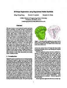
(g) Scan from G7 Fig. 6: Each image represents the reflectance of one of the acquired scans for each group used in our experiments.
4. Experimental Results 4.1. Test Data and Evaluation Criteria Our proposed automatic registration algorithms using linear and planar features were evaluated on a set of real scan data acquired by different types of scanners. In total, we tested 7 groups of scans {G k }7k =1 and each group of scans was acquired from the same scene. The groups {G k }5k =1 were acquired from 5 different indoor laboratory rooms, which consist of 5, 5, 2, 7 and 4 scans, respectively. The groups G 6 and G 7 were acquired from the train station Gare de Lyon in Paris (group G 6 from indoor and group G 7 from outdoor), which consist of 4 and 5 scans, respectively. Fig. 6 depicts the type of environment for each group. In particular we used a Z+F IMAGER 5006 laser rangescanner for G 2 , G 3 and G 5 , a Z+F IMAGER 5006i for G1 and G 4 , and a Z+F IMAGER 5003 for G 6 . For the outdoor environment of G 7 we used a RIEGL LMS-Z420i laser range-scanner. The accuracy of a point acquired by the Z+F IMAGER 5003 (5006 and 5006i) laser scanner is 3mm (1mm) along the laser-beam direction at a maximal
12
distance of 50m from the scanner. The accuracy of the RIEGL LMS-Z420i laser scanner is 10mm at 50m. This scanner can measure objects from 2m up to 1000m. Notice that the laser scanner measurement error increases with the distance, i.e., the sampling density of far surfaces is lower than that of close surfaces. This fact has to be considered when evaluating the accuracy of our registration algorithm on large-scale range scans of groups G 6 and G 7 with respect to small/medium-scale ones of groups {G k }5k =1 . The original resolution of all indoor scans is about 5080 × 2150 and the original resolution of all outdoor scans is 3000 × 666. However, we experimented our algorithms also by sub-sampling range scans at different rates to demonstrate the robustness with respect to different resolutions. A sub-sampling rate of n means that only one point of every n × n grid points is considered. In particular, for groups G1 and G 5 we sub-sampled data with a subsampling rate of 2. In group G 3 , we considered one scan without sub-sampling and another scan with a subsampling rate of 4. Finally, notice that not all pairs of scans in each group have overlapping regions. In this paper, we only consider the pairs of scans in each group having sufficiently large overlap regions ( ≥ 20% ). Our registration algorithms were implemented in C++ on a Windows XP system and integrated into our commercial software JRC 3D Reconstructor18 and all the experiments were executed on a 2.67GHz Intel machine. To evaluate the transformation estimation accuracy of our registration algorithm, we firstly employed our algorithm on selected pairs of scans for all groups to recover a good initial transformation for each scan pair and then applied the ICP optimization algorithm3 to get a well aligned transformation. In this paper, this ICP-optimized transformation would be regarded as the ground truth transformation. In all our experiments, a recovered transformation was regarded as a successful estimation only when the translation error || t′ − t || between the recovered translation t' and the ground truth t is below 5cm (for indoor small/medium-scale scans of groups {G k }5k =1 ) and 50cm (for large-scale scans of groups G 6 and G 7 ). These thresholds were selected based on visual inspection of the tested models and the convergence of the ICP algorithm to the ground ground truth transformation. The rotation angular error between the recovered rotation angles θ′ = [θ x′, θ y′ ,θ z′]Τ and the ground truth θ = [θ x , θ y , θ z ]Τ is defined as || θ′ − θ || . Our registration algorithm was statistically evaluated by running it N run = 50 times on each considered pair of scans. Both the median translation error Dt and the median rotation angular error Dθ of all successful estimations N suc in N run runs are used to evaluate the estimation accuracy of our algorithm. The efficiency and robustness are evaluated by the successful estimation rate S r = N suc N run . In total, we considered 29 pairs of scans from 7 groups of tested scans as shown in Tables 1 and 2.
3D Res. 03, 06 (2010)
evaluated on the aforementioned test data. The main parameters were set as follows. The two threshold parameters for the line roughly matching constraint were set as thθl = 2.5° and β =5 used for adaptively computing thdl . The two parameters for the line precisely matching constraint were set as γ1 =5 and γ2 =2.5. The two parameters for efficient matching of congruent groups of linear features were set as K p = 800 and K g = 30 . The allowed maximal iteration number I max for the RANSAC was set to 1000. Of course, the algorithm was terminated early with less iterations if a good solution with enough matches was found. In addition, our algorithm was terminated when the registration time was above 10 minutes. For each scan, at most 1000 linear features were used in our experiments by removing the shortest ones when the number of extracted features from one scan exceeded 1000. Notice that the same parameter values were used in all the experiments described below.
Fig. 7: Results of our linear feature matching algorithm applied on two pairs of scans in groups G2 (top) and G6 (bottom) representing indoor scenes with small overlap: blue lines from one scan, green lines from another scan and red for matched lines.
4.2. Evaluation on Linear Feature Based Registration The efficiency and robustness of our proposed linear feature based automatic registration algorithm were
Fig. 8: Linear feature based registration results of groups G2 (top) and G6 (bottom): the line segments represented in the same colour were extracted from the same range scan.
3D Res. 03, 06 (2010)
13
Fig. 9: Results of our planar feature matching algorithm applied on two pairs of scans in groups G2 (the two images on the top) and G6 (the two images on the bottom) representing indoor scenes with small overlap. In each pair of scans the matched pairs of planar features are depicted with the same colour. The planar features represented in grey have no matches. Table 1: Performance evaluation of our linear feature based registration algorithm using the probabilistic random selection approach. Meanings of columns: (1) numbers of groups of scans; (2) numbers of linear features extracted from two scans (at most 1000 linear features with largest line lengths were used); (3-4) median numbers N m of best linear feature matches; (5-6) median linear feature matching times t (in sec); (7-9) successful estimation rates S r over 50 runs; (10-13) median translation errors Dt (in mm) w.r.t. ground truth; (14-17) median rotation angular errors Dθ (in degree) w.r.t. ground truth. Note that M denotes the number of randomly selected linear features for initial transformation estimation in RANSAC and the symbol ★ denotes that registration between two scans failed. G
1
2
3
4
5
6
7
t
Sr (%) M=3
M=4
M=2
M=3
M=4
M=2
Dθ (°) M=3 M=4
594
98
100
100
0.8
0.8
1.1
0.07
0.08
601
100
100
92
1.5
1.4
1.6
0.12
0.10
0.14
84
385
98
100
100
0.8
0.7
0.8
0.11
0.11
0.10
309
451
603
40
100
51
2.4
2.4
3.7
1.23
0.38
0.97
367
333
602
53
95
54
2.5
2.5
2.6
0.28
0.25
0.31
52
66
238
95
100
100
1.2
0.9
1.1
0.11
0.06
0.19
327
311
222
604
83
100
23
0.5
0.7
2.1
0.04
0.03
0.06
414
137
126
565
57
100
95
0.6
0.5
1.3
0.03
0.03
0.12
328
388
122
127
574
53
100
97
0.5
0.5
0.7
0.03
0.04
0.05
357
346
459
117
111
343
78
100
100
0.3
0.2
0.6
0.02
0.01
0.03
168
272
288
162
243
604
60
92
77
0.9
1.6
1.6
0.06
0.08
0.10
290×119
63
64
58
23
39
207
100
100
100
0.7
0.5
0.7
0.13
0.10
0.12
400×577
159
165
178
28
65
170
100
100
100
0.1
0.2
0.2
0.02
0.02
0.02
577×564
153
155
203
50
90
346
100
100
100
0.3
0.3
0.4
0.03
0.03
0.07
564×553
127
136
163
53
99
601
100
100
100
0.4
0.3
0.8
0.04
0.04
0.05
553×557
199
208
224
22
39
130
100
100
100
0.3
0.3
0.3
0.02
0.02
0.03
557×594
175
180
207
42
67
249
100
100
100
0.1
0.1
0.3
0.04
0.04
0.04
594×436
121
127
154
54
55
442
100
100
100
0.4
0.4
0.7
0.03
0.03
0.03
879×1000
164
220
49
293
304
602
60
90
26
1.2
1.6
3.3
0.11
0.15
0.24
1000×834
296
305
107
107
94
604
60
97
13
0.8
1.3
2.4
0.06
0.05
0.19
834×587
79
102
82
584
600
602
68
97
13
2.2
1.9
3.9
0.12
0.13
0.24
1000×1000
140
197
225
306
601
605
90
97
56
3.8
3.3
9.3
0.05
0.04
0.20
1000×1000
236
278
292
96
282
606
90
100
74
1.2
1.3
2.8
0.10
0.12
0.18
1000×1000
105
125
162
241
601
604
23
54
62
3.9
3.7
13.9
0.04
0.07
0.17
1000×1000
106
155
242
256
601
604
75
92
49
4.1
5.3
13.6
0.09
0.10
0.18
Nm M=2
M=3
457×398
125
126
457×379
87
88
398×379
116
121
398×500
52
379×500
51
500×507
M=4
(secs)
Dt (mm)
M=2
Features
M=2
M=3
M=4
113
111
103
100
174
202
125
60
70
83
52
74
89
89
129
1000×1000
196
208
1000×1000
294
292
1000×1000
241
1000×1000 1000×1000
0.09
110×197
★
★
★
★
★
★
0
0
0
★
★
★
★
★
★
197×171
13
8
★
173
600
★
100
3
0
17.6
16.7
★
0.17
0.11
★
171×182
★
★
★
★
★
★
0
0
0
★
★
★
★
★
★
182×213
★
13
13
★
600
604
0
10
8
★
32.1
34.6
★
0.47
0.63
Table 1 shows that by setting M = 3 our algorithm usually produced more robust transformations than setting M = 2 and M = 4 (i.e., similar or higher successful
estimation rates Sr in most cases). On the one hand by using M = 2 the recovery of the initial transformation becomes very sensitive to symmetries and noise in
14
3D Res. 03, 06 (2010)
measurement, edge detection and feature extraction, as explained in Section 2.2.1. On the other hand by considering high values of M , e.g., M = 4 , the probability to find congruent groups of matched features in the overlapping area of the models decreases. This effect is particularly evident when the overlapping ratio between two scans is rather small, e.g., about 20-30% as for groups G 5 and G 6 . Most of median translation errors Dt are within 1mm for indoor data {G k }5k =1 and 5cm for group G 6 while most of median rotation angular errors Dθ are within 0.1° for {G k }6k =1 . These values are well suitable for further successful ICP optimization. On models of the group G 7 our algorithm almost always failed due to the large number of mismatches and symmetries present in the extracted features. However, this result outperformed that obtained by using the uniform random (basic RANSAC) selection approach, which was never able to recover the correct transformation. A comparison of the two different RANSAC approaches is shown in Fig. 10, where the four top figures show the histograms of the successful
RANSAC iteration numbers in which good congruent sets of 3 matched linear features were found. The histograms regarding the probability-based RANSAC approach (on the right) clearly show higher frequencies than those regarding the basic RANSAC approach (on the left) and are also more concentrated towards the y -axis (caused by the fact that the algorithm stopped with good estimates before the iteration I max ), meaning that the probability-based RANSAC approach is more efficient in selecting good matches for testing than the basic RANSAC approach. The initial gradually increased trend of the probability-based RANSAC histograms indicates that the procedure of updating the feature pairs matching probabilities increases the chances to find good matches in the next iterations. Fig. 7 shows the results of our linear feature matching algorithm applied on two pairs of scans in groups G 2 (top) and G 6 (bottom) representing indoor scenes with small overlap. The scene registration results of groups G 2 (top) and G 6 (bottom) by using linear feature matching algorithm are shown in Fig. 8.
Table 2: Performance evaluation of our registration algorithm based on planar features using both the uniform ( U R ) and probabilistic ( PR ) random selection approaches. Meanings of columns: (1) numbers of groups of scans; (2) numbers of planar features extracted from two scans; (3-4) median numbers N m of best planar feature matches; (5-6) median planar feature matching times t (in sec); (7-9) successful estimation rates t over 50 runs; (9-10) median translation errors Dt (in mm) w.r.t. the ground truth; (11-12) median rotation angular errors Dθ (in degree) w.r.t. the ground truth. The results reported were obtained by setting the parameter M = 3 , i.e., our algorithm recovered the transformation by matching congruent sets of three planar features.
G
1
2
3
4
5
6
7
Planar
t (secs)
Features
UR
PR
UR
PR
UR
PR
Dt (mm) UR PR
426×432
173
174
111
144
98
100
0.18
426×364
103
103
128
142
97
100
432×364
163
163
54
83
100
100
432×365
103
102
149
244
97
364×365
40
58
144
209
76
365×402
124
124
59
89
372×512
126
126
13
512×508
168
150
13
512×501
164
164
11
Nm
Sr (%)
Dθ (°) UR
PR
0.23
0.027
0.030
0.28
0.11
0.013
0.011
0.07
0.07
0.011
0.012
100
0.26
0.23
0.085
0.081
100
0.43
0.44
0.040
0.041
100
100
0.22
0.22
0.020
0.020
18
99
100
0.10
0.10
0.006
0.006
18
98
100
0.19
0.19
0.011
0.011
20
100
100
0.17
0.17
0.013
0.013
508×501
234
256
7
10
100
100
0.09
0.09
0.010
0.007
501×483
178
178
10
15
99
100
0.08
0.08
0.008
0.008
101×28
17
16
2
3
100
100
0.15
0.14
0.043
0.043
225×238
111
112
6
10
100
100
0.06
0.06
0.003
0.003
238×237
88
89
6
13
100
100
0.06
0.06
0.007
0.007
237×294
76
76
8
34
100
100
0.11
0.11
0.009
0.008
294×262
124
124
9
24
100
100
0.08
0.08
0.003
0.003
262×277
109
109
8
21
100
100
0.08
0.08
0.009
0.008
277×190
67
67
6
15
100
100
0.09
0.09
0.013
0.010
221×86
36
36
6
8
100
100
0.16
0.15
0.034
0.033
86×179
33
34
7
11
100
100
0.23
0.23
0.013
0.014
179×187
28
29
50
88
66
100
0.21
0.19
0.035
0.034
1000×515
127
111
52
60
100
100
0.33
0.33
0.009
0.009
515×497
132
133
24
41
100
100
0.46
0.46
0.041
0.041
497×575
8
72
33
38
62
90
0.80
0.77
0.017
0.016
609×575
98
88
47
52
100
100
0.32
0.31
0.021
0.020
96×92
22
22
9
10
100
100
11.24
9.75
0.055
0.059
92×197
21
22
16
19
100
100
8.52
3.38
0.099
0.069
197×201
8
10
52
22
2
35
30.01
3.51
0.303
0.038
197×115
15
15
19
17
71
86
2.19
3.32
0.048
0.055
3D Res. 03, 06 (2010)
15 Linear features
Planar features
Fig. 10: Comparison of the different versions of our matching algorithm: the basic RANSAC approach (blue) and the probability-based RANSAC (red). The figures show the histograms of the successful RANSAC iteration numbers in which good congruent sets of 3 matched features w.r.t. the ground truth transformations were selected for testing in the RANSAC loop. The first four figures on the top show the results of our algorithm using linear features, while the remaining ones using planar features. In each group of four histograms, those on the top regards the small/medium-scale scans (groups {Gk }5k =1 ), while those on the bottom the large-scale scans (groups G6 and G7 ). The abscissa represents the frequency of the successful RANSAC iteration numbers.
4.3. Evaluation on Planar Feature Based Registration In this section we present the results of our proposed planar feature based automatic registration algorithm. The main algorithm parameters were set as follows. The two threshold parameters for the plane roughly matching constraint were set as thθp = 2.5° and κ = 5 used for adaptively computing thdp . The two parameters for the plane precisely matching constraint were set as ρ1 = 5 and ρ2 = 2.5 . The two parameters for efficient matching of congruent groups of planar features were set as K p = 500
and K g = 30 . We set M = 3 , i.e., our algorithm recovered the transformation by matching congruent sets of three planar features. The same RANSAC termination conditions as in linear feature based registration were used here. The same parameter values were used in all the experiments described below. Table 2 shows the results achieved by our method using planar features on the same test data used in Table 1. The planar feature matching times range from 3 to 244 seconds (most in 1 minute), mainly depending on the numbers of planar features and the amount of matched planar features.
16
Similarly to Table 1 the times reported include: (1) the time of computing the normal angles and shortest distances of all pairs of planar features to be matched, (2) the time for building the codebook for searching similar planar features (which can be computed once for each scan in practice), and (3) the time taken to perform the RANSAC iterations for planar feature matching. The time spent for planar range segmentation33, which was around 2 minutes for each scan, is not included. Most of median translation errors Dt are within 0.5mm for groups {G k }6k =1 and 10mm for group G 7 , which are well suitable for further successful ICP optimization. In most cases, the transformation recovered by the planar feature matching algorithm was very close to the ground truth, and its accuracy was higher than that achieved by using the linear feature matching algorithm. From Table 2 we observed that by using the probabilistic random selection approach our algorithm usually produced more robust and accurate transformations than using the uniform random selection approach (i.e., similar or higher successful estimation rates Sr , and similar or smaller median translation errors Dt and median rotation angular errors Dθ in most cases), especially in group G 7 . A comparison of the two different RANSAC approaches is shown in Fig. 10, where the last four figures on the bottom show the histograms of the successful RANSAC iteration numbers in which good congruent sets of 3 matched planar features were found. A similar behaviour as for the linear features was observed here. Thus, for both linear and planar features the probability-based RANSAC approach outperformed the basic RANSAC approach by quickly recovering more relevant congruent sets of features.
3D Res. 03, 06 (2010)
The results shown in Table 2 were obtained by refining the transformation using the second iterative optimization approach (based on the point-to-point error metric). We also tested our planar feature matching algorithm on the same data with the first iterative optimization approach (based on the point-to-plane error metric). We found that the first approach is little faster and less accurate than the second one (i.e., little larger Dt and Dθ ). However, the accuracy of the initial transformation obtained with the first iterative approach is much better than that obtained with the linear feature matching. Fig. 9 shows the results of our planar feature matching algorithm applied on two pairs of scans in groups G 2 (top) and G 6 (bottom) representing indoor scenes with small overlap. We also evaluated the performance of different feature types by comparing linear and planar features. The results are shown in Fig. 11. In particular the median numbers of iterations and the median execution times using planar features are always smaller than using linear features. Furthermore, for groups G 5 and G 6 the numbers of iterations of the linear feature based registration algorithm are very high and were not reported, since their execution times exceeded the fixed maximal value of 10 minutes. Notice, however, that the initial segmentation of planar features requires more time than extracting linear features from the same acquisition. We also compared the obtained registration results with respect to the ground truth registration. Both median translation errors and median rotation angular errors are lower using planar features than using linear features. Moreover, the median translation errors of the planar feature based algorithm are almost always under the expected accuracy of the laser scanner. This confirms the goodness of the obtained registration.
Fig. 11: Comparison of the different feature types of our matching algorithm using the probability-based RANSAC approach with M = 3 : (top-left) median numbers of iterations required by each group (for groups G6 and G7 we do not show any value using linear features since too many algorithm runs terminated due to the time limit of 10 minutes); (top-right) median execution times of all completed experiments for each group; (bottom) median translation errors (left) and median rotation angular errors (right) w.r.t. the ground truth transformation for each group.
3D Res. 03, 06 (2010)
Our probability-based RANSAC approach shows better effectiveness in matching planar features than linear features. This observation results from analysing Fig. 10, and Tables 1 and 2, in which by using planar features our approach respectively reports higher histogram values close to the y -axis and higher successful estimation rates than using linear features. This fact further justifies the use of our proposed variant of RANSAC approach and planar feature matching method.
17
volumetric feature points to align CT or multi-sensor scans in medical applications. References 1. 2.
5. Conclusions We presented an efficient method to automatically register range scans with different resolutions. Our algorithm automatically aligns two range scans by seeking for the congruent sets of linear or planar features leading to the best estimate of the rigid transformation between the corresponding point clouds. The computed transformation is then further refined using the ICP algorithm. Linear features consist of line segments in ℜ3 , which are detected from edge contours extracted from 2D reflectance images and refined with their 3D information. Planar features are geometrically described by planar patches in ℜ3 , which are computed through hierarchical segmentation of range images in planar regions33. Our method follows the RANSAC approach to find the congruent groups of matched features leading to the best transformation estimate. To make the performance attainable to practical application we introduced a fast matching algorithm using a codebook to efficiently search similar features through adaptive range-queries. We then presented a novel weighting function, which improved the robustness of the transformation recovery method using sets of congruent features. Our weighting function mitigates the effect of inhomogeneous feature sampling densities. We presented a variant of the basic RANSAC approach based on the matching probability of each pair of features. This variant demonstrated improved efficiency and robustness with respect to noise and different scans resolutions. Our matching algorithm is applicable to any types of features by only providing a proximity function and a constrain criterion for the features considered. Its robustness and efficiency were experimentally demonstrated on several challenging range data sets acquired from indoor and outdoor scenes with different scales. Experiments showed that the accuracy, robustness and matching effectiveness of our registration method using planar features are better than that using linear features. With the same input parameters our method using planar features was capable to register all the tested pairs of range scans with an accuracy similar to the acquisition one. Although the planar feature matching algorithm showed smaller matching times, the time required by the planar segmentation (few minutes) is always much higher than the linear feature extraction one (few seconds). As future work we plan to improve the performance of our planar range segmentation and matching algorithm, and to extend our matching framework to other geometric features which are suitable to efficiently register 3D scanned data in specific contexts, e.g., use image-based or
3.
4. 5.
6.
7. 8.
9.
10.
11.
12.
13.
14. 15.
D. Aiger, N. J. Mitra, D. Cohen-Or (2008) 4-Points Congruent Sets for Robust Pairwise Surface Registration, ACM SIGGRAPH S. Arya, D. M. Mount, N. S. Netanyahu, R. Silverman, A. Y. Wu (1994) An Optimal Algorithm for Approximate Nearest Neighbor Searching in Fixed Dimensions, ACM-SIAM Symposium on discrete algorithms P. J. Besl, H. D. McKay (1992) A method for registration of 3-D shapes, IEEE Transactions on Pattern Analysis and Machine Intelligence, 14(2):239–256 John Canny (1986) A Computational Approach to Edge Detection, IEEE Transactions on Pattern Analysis and Machine Intelligence, 8(6):679–698 C. Chao, I. Stamos (2006) Range Image Registration Based on Circular Features, The International Symposium on 3D Data Processing Visualization and Transmission C. Chao, I. Stamos (2005) Semi-automatic Range to Range Registration: a Feature-based Method, International Conference on 3-D Digital Imaging and Modeling (3DIM) Y. Chen, G. Medioni (1992) Object Modeling by Registration of Multiple Range Images, Image & Vision Computing, 10(3):145–155 C. Dold, C. Brenner (2006) Registration of terrestrial laser scanning data using planar patches and image data, International Society for Photogrammetry and Remote Sensing D. Douglas, T. Peucker (1973) Algorithms for the Reduction of the Number of Points Required to Represent a Digitized Line or its Caricature, The Canadian Cartographer, 10(2):112–122 M. A. Fischler, R. C. Bolles (1987) Random Sample Consensus: a Paradigm for Model Fitting with Applications to Image Analysis and Automated Cartography, Communications of the ACM, :726–740 M. Franaszek, G. S. Cheok, C. Witzgall (2009) Fast Automatic Registration of Range Images from 3D Imaging Systems Using Sphere Targets, Automation in Construction, 18(3):265–274 N. Gelfand, N. J. Mitra, L. J. Guibas, H. Pottmann (2005) Robust Global Registration, Third Eurographics Symposium on Geometry Processing (SGP) F. Han, Z. W. Tu, S. C. Zhu (2004) Range Image Segmentation by an Effective Jump-Diffusion Method, IEEE Transactions on Pattern Analysis and Machine Intelligence, 26(9):1138–1153 R. I. Hartley, A. Zisserman (2004) Cambridge University Press, Multiple View Geometry in Computer Vision, ISBN: 0521540518, Second edition R. Hesami, A. Bab-Hadiashar, R. HosseinNezhad (2010) Range Segmentation of Large Building
18
16. 17.
18. 19.
20.
21.
22. 23.
24.
25.
26.
27.
3D Res. 03, 06 (2010)
Exteriors: a Hierarchical Robust Approach, Computer Vision and Image Understanding, 114(4):475–490 F. H. Daniel, M. Hebert (2003) Fully Automatic Registration of Multiple 3D Data Sets, Image and Vision Computing, 21(7):637–650 A. E. Johnson, M. Hebert (1999) Using Spin Images for Efficient Object Recognition in Cluttered 3D Scenes, IEEE Transactions on Pattern Analysis and Machine Intelligence, 21(5):433–449 Joint Research Centre of European Commission, JRC 3D Reconstructor, http://www.reconstructor.it B. Kamgar-Parsi, B. Kamgar-Parsi (2004) Algorithms for Matching 3D Line Sets, IEEE Transactions on Pattern Analysis and Machine Intelligence, 26(5):582–593 Z. Z. Kang (2008) Automatic Registration of Terrestrial Point Cloud Using Panoramic Reflectance Images, International Society for Photogrammetry and Remote Sensing Kok-Lim Low (2004) Linear Least-Squares Optimization for Point-to-Plane ICP Surface Registration. Technical report, TR04-004, Department of Computer Science, University of North Carolina at Chapel Hill D. G. Lowe (2004) Distinctive Image Features from Scale-Invariant Keypoints, International Journal of Computer Vision, 60(2):91–110 A. Makadia, A. Patterson (2006) IV and Daniilidis, K. Fully Automatic Registration of 3D Point Clouds, IEEE Conference on Computer Vision and Pattern Recognition (CVPR) C. Matabosch, J. Salvi, D. Fofi, F. Meriaudeau (2005) Range image Registration for Industrial Inspection, Machine Vision Applications in Industrial Inspection XIII, pages 216–227 V. Nguyen, S. Gächter, A. Martinelli, N. Tomatis, R. Siegwart (2007) A Comparison of Line Extraction Algorithms Using 2D Range Data for Indoor Mobile Robotics, Autonomous Robots, 23(2):97–111 M. Pollefeys, L. Van Gool, M. Vergauwen, F. Verbiest, K. Cornelis, J. Tops, R. Koch (2004) Visual modeling with a hand-held camera, International Journal of Computer Vision, 59(3):207–232 T. Rabbani, F. van den Heuvel (2005) Automatic Point Cloud Registration Using Constrained Search for Corresponding Objects, 7th Conference on Optical 3-D Measurement Techniques
28. S. Rusinkiewicz, M. Levoy (2001) Efficient Variants of the ICP Algorithm, International Conference on 3D Digital Imaging and Modeling (3DIM) 29. A. Sampath, J. Shan (2010) Segmentation and Reconstruction of Polyhedral Building Roofs From Aerial Lidar Point Clouds, IEEE Transactions on Geoscience and Remote Sensing, 48(3):1554–1567 30. I. Stamos, M. Leordeanu (2003) Automated Featurebased Range Registration of Urban Scenes of Large Scale, IEEE Conference on Computer Vision and Pattern Recognition (CVPR) 31. Umeyama Shinji (1991) Least-Squares Estimation of Transformation Parameters Between Two Point Patterns, IEEE Transactions on Pattern Analysis and Machine Intelligence, 13(4):376–380 32. L. Wang, S. You, U. Neumann (2008) Supporting Range and Segment-based Hysteresis Thresholding in Edge Detection, International Conference on Pattern Recognition (ICIP) 33. J. Yao, P. Taddei, M. R. Ruggeri, V. Sequeira (2010) Complex and Photo-realistic Scene Representation Based on Range Planar Segmentation and Model Fusion, The International Journal of Robotics Research, submitted 34. Jian Yao (2006) PhD thesis, The Chinese University of Hong Kong, Shatin, N.T. , Hong Kong, P.R. China, Modeling and rendering from multiple views, Adviser-Cham, Wai-Kuen 35. Jian Yao, Cham, Wai-Kuen (2007) Robust multi-view Feature Matching from Multiple Unordered Views, Pattern Recognition, 40(11):3081–3099 36. L. Yu, D. Zhang, E. Holden (2008) A Fast and Fully Automatic Registration Approach Based on Point Features for Multi-source Remote-sensing Images, Computers and Geosciences, 34(7):838–848 37. A. Zaharescu, E. Boyer, K. Varanasi, R. Horaud (2009) Surface Feature Detection and Description with Applications to Mesh Matching, IEEE Conference on Computer Vision and Pattern Recognition (CVPR) 38. Wei Zhang, Jian Yao, Wai-Kuen Cham (2010) 3D Modeling from Multiple Images, The Seventh International Symposium on Neural Networks (ISNN 2010), pages 97–103 39. Z. Zhang, O. D. Faugeras (1991) Determining motion from 3D line segment matches: a comparative study, Image Vision Computing, 9(1):10–19