We minimize (1) by the L-BFGS algorithm with respect to the pa- rameters a. Regularization is added to avoid non-uniqueness [16], yielding. JS (aF G) = â MIL(f ...
AUTOMATIC SIMULTANEOUS SEGMENTATION AND FAST REGISTRATION OF HISTOLOGICAL IMAGES Jan Kybic, Jiˇr´ı Borovec Czech Technical University in Prague, Czech Republic ABSTRACT We describe an automatic method for fast registration of images with very different appearances. The images are jointly segmented into a small number of classes, the segmented images are registered, and the process is repeated. The segmentation calculates feature vectors on superpixels and then it finds a softmax classifier maximizing mutual information between class labels in the two images. For speed, the registration considers a sparse set of rectangular neighborhoods on the interfaces between classes. A triangulation is created with spatial regularization handled by pairwise spring-like terms on the edges. The optimal transformation is found globally using loopy belief propagation. Multiresolution helps to improve speed and robustness. Our main application is registering stained histological slices, which are large and differ both in the local and global appearance. We show that our method has comparable accuracy to standard pixel-based registration, while being faster and more general. Index Terms— image registration, image segmentation, mutual information, loopy belief propagation 1. INTRODUCTION The motivation of our work is registration of large histological slices (see Fig. 1,2). Many different stains exist to visualize different aspects of the cell structure and the presence of various proteins and other biomarkers. Since only a limited number of stains can be used in a single slice, to obtain a complete information about a specific tissue location, the slices must be registered [1]. There can be large differences in the global appearance. Not only the color is different but also different objects are visible. Moreover, because of distance between slices, the small details small-scale details do not correspond either. Other applications include fast multimodal registration in medical imaging or remote sensing. Our strategy is first to simultaneously segment the two images by learning two independent classifiers so that the segmentation they produce is as similar as possible. Then, we quickly register the two segmentations by aligning the class contours using a sparse set of control points. The segmentation and registration can be viewed as alternative minimizations of the same criterion, the mutual information on labels (MIL). The algorithm is fast and parallelisable. 1.1. Related work Methods used for aligning histology slices include global pixelbased methods [1–3], local search methods [4,5], and features-based methods [6]. However, these approaches assume the same appearance of all images. The project was partially supported by Czech Science Foundation under project P202/11/0111 and the Grant Agency of the Czech Technical University in Prague, grant No.SGS12/190/OHK3/3T/13.
Methods combining segmentation and registration find object contours by level set methods [7,8], or by thresholding [9], formulate a joint criterion minimized by GraphCut [10], or register segmented objects based on shape descriptors [11]. Image registration by discrete minimization was proposed by [12] and others on a dense grid. 2. METHOD Given a reference image F and a moving image G on a pixel grid Ω, we want to find a transformation T , such that a point r in image F corresponds to point r′ = T (r) in image G. Instead of registering directly the images F and G, we register their segmentations f and g. We alternate segmentation (Section 3) and registration (Section 4) until convergence. In both steps, we minimize the same criterion J, the mutual information between the two segmentations (Section 2.1): J(f, g, T ) = − MIL(f, T ◦ g) + R
(1)
with f = Ψf F, g = Ψg G, where f and g are soft segmentations, i.e. fk (j) is a probability that a pixel j in image F belongs to class k, and Ψf is a parameterized class probability model (Section 3.1). When needed, hard segmentation is obtained as fˇk (j) = Jk = arg maxl fl (j)K. The symbol R represents regularization (see equations 5,11). Image G should be treated analogously. 2.1. Mutual information of labels Mutual information of labels (MIL) is similar to standard MI [13,14] X pk,l (2) pk,l log MIL(f, g) = pk pl k,l P P with pk = l pk,l and pl = k pk,l . The pk,l is a probability that at the same location, the class in F is k and the class in G is l. 1 X pk,l = fk (j)gl (j) (3) |Ω| j∈Ω Compared to standard MI, the number of bins (classes) is much smaller. Therefore, MIL is more robust, faster to evaluate and needs less input samples. We choose to consider only integer displacements during registration, T (x) ∈ Ω, so no interpolation is needed. 3. SEGMENTATION The segmentation assigns each pixel a class {1, 2, . . . , L}, where L is given. It starts by calculating SLIC superpixels [15], Si ⊂ Ω. ˜i See Fig.1 for examples. In the second step, a descriptor vector x is calculated for each superpixel Si . The descriptors are application P ˜ i = |S1i | j∈Si F (j) to be dependent; we found simple means x sufficient. Note that we work with�colour, � three channel images. For ˜i . further convenience, we set xi = 1 x
(a)
(b)
(c)
(d)
(e)
(f)
(g)
(h)
(a)
(b)
(c)
(d)
(e)
(f)
(g)
(h)
Fig. 1. Top two rows: Histology slices of rat kidney stained with H&E and PanCytokeratin. Bottom two rows: Histology slices of human prostate [1] stained with H&E and PSAP. We show the input images (a,e), the superpixels (b, yellow lines) and the segmentation and triangulated mesh (f) of (a) with big red dots for control points C. Images (c,g) show the position of the control points C in the moving image before and after the first iteration, overlaid over the segmentation of (e). Images (d,h) show the overlaid images before and after registration.
3.1. Softmax regression d
L
The class probability model Ψ : R → R takes a descriptor vector xi and produces the probabilities zi,k for each class k and superpixel i, corresponding to a soft pixel-level segmentation fk (j) = zi,k , with j ∈ Si . We use a linear softmax regression [16], parameterized by vectors of coefficients ak ∈ Rd for class k. � exp aTk xi zi,k = PL (4) � T l=1 exp al xi 3.2. Optimization We minimize (1) by the L-BFGS algorithm with respect to the parameters a. Regularization is added to avoid non-uniqueness [16], yielding β JS (aF G ) = − MIL(f, T ◦ g) + kaF G k2 (5) 2L � � with aF G = aF aG , where aF , aG are class model parameters (from (4)) for images F and G, respectively. The probability pk,l (3)
to find MIL is evaluated directly on superpixels as 1 X F G si,j zi,k zj,l pk,l = |Ω| (i,j) P with superpixel overlaps si,j = r∈Si JT (r) ∈ Sj K. 3.3. Initialization Because the criterion (5) is not convex, a reasonable initialization for the parameters a is required. We choose randomly L positions v1 , . . . vL in the image, and find sets of superpixels UkF and UkG within a small radius rinit from vk in F and from T (vk ) in G, respectively. Using L-BFGS, we find such coefficients aF G , so that the superpixels in UkF and UkG are in class k by minimizing a sum of standard softmax cost functions for the two images JI (aF G ) = LF + LG + L• = PL
k=1
1 P
β kaF G k2 2L L X X
• i∈Uk
wiF
k=1
• i∈Uk
(6) • wi• log zi,k
(7)
where wi = |Si | is the superpixel size. Once the initial aF G is found, we continue by minimizing (5). We repeat the random initialization Ninit times and the best aF G in terms of J (1) is retained.
We use belief propagation [19], which sends messages µti→ (yj ) = min yi
�ω
ij
2
k(yi − ri ) − (yj − rj )k2 + Di (yi ) +
4. REGISTRATION
X
µt−1 s→i (yi )
�
(12)
s6=j
The registration minimizes a sum of the MIL data criterion and a smoothness term using loopy belief propagation. The key observation is that as T varies, the only contributions to the change of MIL(f, T ◦ g) come from the boundaries between classes. Furthermore, as T is smooth, it is sufficient to describe it by its value yi = T (ri ) at a sparse set of control points ri ∈ C. Control points are located at class boundaries and are pruned to be at least ε pixels apart. Once the new control point positions yi = T (ri ) are found, the transformation T can be interpolated everywhere using either bilinear interpolation on each triangle, or the Clough-Tocher scheme [17], if a C 1 continuity is required. 4.1. Data criterion The contribution Di of small neighborhoods Ωi of size h × h pixels around each control point is X pk,l (8) p˜k,l log Di (yi ) = − pk pl k,l
where pk,l is calculated from (3) in the whole image Ω, while p˜k,l is calculated from the corresponding neighborhood Ωi . We allow only integer yi and limit the maximum displacement, kyi − ri k∞ ≤ d. Then Di is precalculated for all ri ∈ C. For convenience, we define Di = 0 for ri 6∈ C. 4.2. Regularization We triangulate1 the points C (see Fig.1b), providing an augmented set of control points C ′ ⊇ C and a set of undirected edges E ⊆ C ′ × C ′ . The regularization consists of pairwise spring-like terms [6, 18], penalizing differences in relative control point displacements U=
1 X ωij k(yi − ri ) − (yj − rj )k2 2
(9)
(i,j)∈E
For small deformations such spring model approximates the behavior of a thin membrane [18] with a Poisson ratio ν = 1/3 if we set the contribution to the weights ωij from each triangle as ωij = λ
kri − rj k2 1� 3 cot2 α + 8A 2
(10)
where λ is the Lam´e’s first parameter, A is the triangle area and α is the angle oposite to the edge ij. 4.3. Belief propagation The registration minimizes a sum of contributions (8) with the regularization (9) with respect to yi for ri ∈ C ′ . JR =
X
ri ∈C
Di (yi ) +
1 X ωij k(yi − ri ) − (yj − rj )k2 (11) 2 (i,j)∈E
1 Using the MeshPy library, software/meshpy/
http://mathema.tician.de/
for (i, j) ∈ E until convergence. Then the estimated displacement � P is extracted as y∗j = arg maxyj Dj (yj ) + i µti→j (yj ) The computational complexity of belief propagation is O(|E|d2 ) per iteration, which can be prohibitive for large d. A speed-up can be achieved by a coarse to fine multiresolution strategy, which requires filtering and downsampling around the control points and a modification of the way the messages are calculated to incorporate the starting point from the previous level. 4.4. Affine initialization If the deformation to be found is large, it is preferable to first find an affine transformation TA minimizing the MIL data criterion. A simple non-iterative method works sufficiently well: We find the locally optimal displacements P y∗i = arg miny Di (y) and calculate a least squares fit minimizing i kTA (ri ) − y∗i k2 by solving a linear system of equations. Second, we warp the image G′ = TA ◦ G (only the superpixel map S G needs to be warped) and perform the procedure as described above to find an elastic transformation TE between F and G′ . The final transformation is a composition T = TE ◦ TA . 5. RESULTS Figure 1 shows the ASSAR intermediate and final results for two examples—differently stained nearby histological slices of rat kidney and human prostate of about 2000 × 2000 pixels. We use the following parameters in both examples: Ninit = 10, rinit = 5, K = 4, λ = 10, h = 10, d = 3, β = 10−3 , ε = 20, and 1000 superpixels. Several iterations of the ASSAR algorithm are performed, each taking about 30 s. The resulting deformation is usable already after the first iteration, further improvements are small. We have compared the speed, robustness and accuracy of ASSAR with B-spline based elastic image registration implemented in bUnwarpJ [9] using sum of squared differences (SSD) and Elastix [20] using mutual information (MI). We have also applied a coarse feature-based affine pre-registration using SURF and RANSAC as implemented in OpenCV; this method is denoted OpenCV+Elastix. The comparison is done on 34 histology image pairs with 40∼90 manually identified landmarks per image (see Figure 2). We calculate the landmark registration error and consider registration a success if the median error decreases by at least 50 %. We report the execution time, mean and median landmark error and the percentage of successful runs in Table 1. We see that ASSAR has the highest success rate among all tested methods and it is also the fastest one, in spite of being currently implemented in Python. Only OpenCV+Elastix is more accurate but also much slower. 6. CONCLUSIONS We have presented a new general image registration method for images with very different local and global appearances. The method is competitive with traditional pixel-based methods in terms of accuracy. This indicates that the class label probably captures most
method bUnwarpJ Elastix OpenCV+Elastix ASSAR
time 401 515 764 130
mean err. 64 54 23 36
median err. 50 45 12 17
success rate 50% 67% 88% 91%
Table 1. Comparison of registration methods. We show the execution time in seconds, the mean and median registration error in pixels, and percentage of successful runs.
156.7 px
30.4 px
17.5 px
42.5 px
7.8 px
8.8 px
145.3 px (a)
18.9 px (b)
7.7 px (c)
Fig. 2. Reference image with manually identified landmark positions in both images connected by red lines (a); the target image with true and calculated landmark positions by ITK (b), and ASSAR (c). Means of the landmark registration errors in pixels are shown below each image; bold denotes the best result.
of the information common between the images. ASSAR is also robust, with a large basin of attraction. Most importantly, by considering only a small fraction of the image pixels, an optimized implementation of ASSAR has the potential of being many times faster than standard pixel-based method. ASSAR could also be combined with existing methods by for example providing a fast initialization to a more accurate but less robust and slower standard pixel-based method.
References [1] G. Metzger, S. Dankbar, J. Henriksen, A. Rizzardi, N. Rosener, and S. Schmechel, “Development of multigene expression signature maps at the protein level from digitized immunohistochemistry slides,” PLoS ONE, vol. 7, no. 3, pp. e33520, 2012. [2] M. Auer, P. Regitnig, and G. Holzapfel, “An automatic nonrigid registration for stained histological sections.,” IEEE Trans. Im. Processing, vol. 14, no. 4, pp. 475–86, 2005. [3] Jiˇr´ı Borovec, Jan Kybic, Michal Buˇsta, Carlos Ortiz-de Solorzano, and Arrate Mu˜noz-Barrutia, “Registration of mul-
tiple stained histological sections,” in Proceedings of 2013 IEEE International Symposium on Biomedical Imaging: From Nano to Macro, 3 Park Avenue, 17th Floor, New York, USA, April 2013, IEEE, pp. 1022–1025, IEEE Computer Society Press. [4] M. Chakravarty, G. Bertrand, C. Hodge, A. Sadikot, and L. Collins, “The creation of a brain atlas for image guided neurosurgery using serial histological data,” NeuroImage, vol. 30, no. 2, pp. 359 – 376, 2006. [5] H. Hufnagel, X. Pennec, G. Malandain, H. Handels, and N. Ayache, “Non-linear 2D and 3D registration using block-matching and B-splines,” in Bildverarbeitung f¨ur die Medizin, pp. 325– 329. Springer, 2005. [6] S. Saalfeld, R. Fetter, A. Cardona, and P. Tomancak, “Elastic volume reconstruction from series of ultra-thin microscopy sections,” Nature Methods, , no. 9, pp. 717–720, 2012. [7] A. Yezzi, L. Z¨ollei, and T. Kapur, “A variational framework for integrating segmentation and registration through active contours,” Med. Im. Anal., , no. 7, pp. 171–185, 2003. [8] F. Wang and B. C. Vemuri, “Simultaneous registration and segmentation of anatomical structures from brain MRI,” in MICCAI, 2005, pp. 17–25. [9] I. Arganda-Carreras, R. Fern´andez-Gonz´alez, A. Mu˜noz Barrutia, and C. Ortiz-De-Solorzano, “3D reconstruction of histological sections: Application to mammary gland tissue.,” Microscopy research and technique, vol. 73, no. 11, pp. 1019–29, 2010. [10] D. Mahapatra and Y. Sun, “Joint registration and segmentation of dynamic cardiac perfusion images using mrfs,” in MICCAI, 2010, pp. 493–501. [11] H. Gonc¸alves, J. A. Gonc¸alves, and L. Corte-Real, “HAIRIS: a method for automatic image registration through histogrambased image segmentation.,” IEEE Trans. Im. Processing, vol. 20, no. 3, pp. 776–789, 2011. [12] B. Glocker, N. Komodakis, G. Tziritas, N. Navab, and N. Paragios, “Dense image registration through MRFs and efficient linear programming,” Med. Im. Anal., vol. 12, no. 6, pp. 731–741, 2008. [13] P. Viola and W. M. Wells, “Alignment by Maximization of Mutual Information,” Int. J. Comp. Vision, vol. 24, no. 2, pp. 134– 154, 1997. [14] J. Pluim, J. Maintz, and M. Viergever, “Mutual-informationbased registration of medical images: A survey,” IEEE Trans. Med. Imaging, vol. 22, no. 8, pp. 986–1004, 2003. [15] R. Achanta, A. Shaji, K. Smith, A. Lucchi, P. Fua, and S. S¨usstrunk, “SLIC superpixels compared to state-of-the-art superpixel methods,” IEEE Trans. Pat. Anal. Mach. Intel., vol. 34, no. 11, pp. 2274–2282, 2012. [16] T. Hastie, R. Tibshirani, and J. Friedman, The Elements of Statistical Learning, Springer, 2001. [17] R. W. Clough and J. L. Tocher, “Finite element stiffness matrices for analysis of plates,” in Proceedings of the conference on matrix methods in structural mechanics, 1965. [18] H. Delingette, “Triangular springs for modeling nonlinear membranes,” IEEE Trans. Vis. Comp. Graphics, vol. 14, no. 2, 2008. [19] P. Felzenszwalb and D. Huttenlocher, “Efficient belief propagation for early vision,” Int. J. Comp. Vision, vol. 70, no. 1, pp. 41–54, 2006. [20] S. Klein, M. Staring, and K. Murphy, “Elastix: a toolbox for intensity-based medical image registration,” Medical Imaging, IEEE, vol. 29, no. 1, 2010.