AUTOTAGGING MUSIC USING SUPERVISED MACHINE LEARNING Douglas Eck Sun Labs Sun Microsystems Burlington, Mass, USA
[email protected]
Thierry Bertin-Mahieux Univ. of Montreal Dept. of Comp. Sci. Montreal, QC, Canada
[email protected]
ABSTRACT Social tags are an important component of “Web2.0” music recommendation websites. In this paper we propose a method for predicting social tags using audio features and supervised learning. These automatically-generated tags (or “autotags”) can furnish information about music that is untagged or poorly tagged. The tags can also serve to smooth the tag space from which similarities and recommendations are made by providing a set of comparable baseline tags for all tracks in a recommender system. 1 INTRODUCTION Social tags are a key part of “Web 2.0” technologies and have become an important source of information for recommendation. In the domain of music, websites such as Last.fm 1 use social tags as a basis for recommending music to listeners. In this paper we propose a method for predicting social tags using audio feature extraction and supervised learning. These automatically-generated tags (or “autotags”) can furnish information about music for which good, descriptive social tags are lacking. The tags can also serve to smooth the tag space from which similarities and recommendations are made by providing a set of comparable baseline tags for all tracks in a recommender system. In this paper we investigate the automatic generation of tags with properties similar to those generated by social taggers. Specifically we introduce a machine learning algorithm that takes as input acoustic features and predicts social tags mined from the web (in our case, Last.fm). The model can then be used to tag new or otherwise untagged music, thus providing a (partial) solution to the cold-start problem. We believe these autotags might also serve to dampen feedback loops which occur when certain songs in a social recommender become over-popular and thus over-tagged. This paper represents preliminary work: we have tested our approach on a sufficient number of tagsets THIS IS THE ORIGINAL 6 PAGE VERSION OF THE PAPER. THE PAPER WAS LATER SHORTENED TO 4 PAGES FOR INCLUSION AT ISMIR. 1 http://last.fm
c 2007 Austrian Computer Society (OCG).
Paul Lamere Sun Labs Sun Microsystems Burlington, Mass, USA
[email protected]
to conclude that the approach has merit. However we have yet to test the output of the model in a social tagging system. Thus we are unable to say at this time how well such an approach will perform with embedding new songs or with “smoothing” recommendations in the event of feedback loops. Our paper is organized as follows: in Section 2 we discuss social tags in more depth, including a discussion of the tag set we built for these experiments. In Section 3 we present an algorithm for autotagging songs based on labeled data acquired on the Internet using data mining techniques. In section Section 4 we present experimental results and also discuss the ability to use model results for visualization. 2 SOCIAL TAGGING Recently, there has been increasing interest in social tagging [8] including the social tagging of music. Music tagging sites such as Last.fm and QLoud 2 allow music listeners to apply free-text labels (tags) to songs, albums or artists. Typically, users are motivated to tag as a way to organize their own personal music collection. A user may tag a number of songs as “mellow” some songs as “energetic” some songs as “guitar” and some songs as “punk” The labels may overlap (a single song may be labeled “energetic” “guitar” and “punk” for example). Typically, a music listener will use tags to help organize their listening. A listener may play their “mellow” songs during the evening meal, and their “energetic” artists while they exercise. The real strength of a tagging system is seen when the tags of many users are aggregated. When the tags created by thousands of different listeners are combined, a rich and complex view of the song or artist emerges. Table 1 show the top 20 tags and frequencies of tags applied to the band “The Shins” Users have applied tags associated with the genre (Indie, Pop, Rock, Emo, Folk etc.), with the mood (mellow, chill), opinion (favorite), style (singersongwriter) and context (Garden State). From these tags and their frequencies we learn much more about “The Shins” than we would from a traditional single genre assignment of “Indie Rock”. Additionally, in previous work [3] it was shown that social tags (in this case from the 2
http://www.qloud.com
freedb CD track listing service at www.freedb.org) can predict canonical music-industry genre with good accuracy. Thus we lose little and gain a lot by moving from genres to tags. For this research, we extracted tags and tag frequencies for over 50,000 artists from the social music website Last.fm using the Audioscrobbler web service [1]. Table 2 shows the distribution of the types of tags for the 500 most frequently applied tags. The majority of tags describe audio content. Genre, mood and instrumentation account for 77% of the tags. This bodes well for using the tags to predict audio similarity as well as using audio to predict social tags. However, there are numerous issues that can make working with tags difficult. Taggers are inconsistent in selecting tags, using synonyms such as “favorite”, “favourite” and “favorites”, “hip hop” “hiphop” and “hiphop”. Taggers use personal tags that have little use when aggregated (“i own it”, “seen live’). Tags can be ambiguous; “love” can mean a romantic song or it can mean that the tagger loves the song. Taggers can be malicious, purposely mistagging items (presumably there is some thrill hearing lounge singer Barry Manilow included in a death metal playlist). Taggers can purposely mistag items in an attempt to increase or decrease the popularity of an item. Although these issues make working with tags difficult, they are not impossible to overcome. Some strategies to deal with these are described in [6]. When social tags are used as a part of collaborative filtering systems, there is also the problem of social feedback loops: a song can become popular simply because a few people start recommending it. This was documented in [10], where a number of artificial music markets were created. Increasing social influence in the system resulted in unequal and unpredictable performance. In short, popular songs become more popular while unpopular songs become more unpopular. Also, in different social influence worlds (as created in the experiment), a particular song might move to #1 or languish at the bottom of the charts. Perhaps related, in the social recommender Last.fm, a song by The Postal Service remained at number one on the charts for 6 months, seemingly due to a user-recommendation feedback loop[7]. A more difficult issue is the uneven coverage and sparseness of tags for unknown songs or artists. Since tags are applied by listeners, it is not surprising that popular artists are tagged much more frequently than non-popular artists. In the data we collected from Last.fm, “The Beatles” are tagged 30 times more often than “The Monkees”. This sparseness is particularly problematic for new artists. A new artist has few listeners, and therefore, few tags. A music recommender that uses social tags to make recommendations will have difficulties recommending new music because of the tag sparseness. This cold-start problem is a significant issue to address if we are to use social tags to help recommend new music. Overcoming the cold-start problem is the primary motivation for this area of research. For new music or sparsely tagged music, we predict social tags directly from the au-
Tag Indie Indie rock Indie pop Alternative Rock Seen Live Pop The Shins Favorites Emo
Freq 2375 1138 841 653 512 298 231 190 138 113
Tag Mellow Folk Alternative rock Acoustic Punk Chill Singer-songwriter Garden State Favorite Electronic
Freq 85 85 83 54 49 45 41 39 37 36
Table 1. Top 20 tags applied to The Shins Tag Type Genre Locale Mood Opinion Instrumentation Style Misc Personal
Frequency 68% 12% 5% 4% 4% 3% 3% 1%
Examples heavy metal, punk French, Seattle, NYC chill, party love, favorite piano, female vocal political, humor Coldplay, composers seen live, I own it
Table 2. Distribution of tag types dio and apply these automatically generated tags (called autotags) in lieu of traditionally applied social tags. By automatically tagging new music in this fashion, we can reduce or eliminate much of the cold-start problem. 3 AN AUTOTAGGING ALGORITHM We now describe a machine learning model which uses the meta-learning algorithm AdaBoost [4] to predict tags from acoustic features. This model is an extension of a previous model [2] which performed well at predicting music attributes from acoustic features: at MIREX 2005 (ISMIR conference, London, 2005) the model won the Genre Prediction Contest and was the 2nd place performer in the Artist Identification Contest. The model has two principal advantages. First it performs automatic feature selection based on a feature’s ability to minimize empirical error. Thus we can use the model to eliminate useless feature sets. Second, it’s performance is linear in the number of inputs. Thus it has the potential to scale well to large datasets. (To be clear: this performance is task dependent and has not been conclusively demonstrated. However it is a motivation for our use of AdaBoost). Both of these properties are general to AdaBoost and are not explored further in this short paper. See [4, 11] for more. 3.1 Acoustic feature extraction We generated MP3s from a subset of the tagged artists described in Section 2. From these MP3s we extracted
several popular acoustic features. Do to space limitations, we do not cover feature extraction in depth here. Please see [2] for details. The features were extracted with high temporal precision to preserve spectral and timbral information. Following the strategy of [2] coarser “aggregate” features were generated by taking means and standard deviations of high-temporal precision features over longer timescales. For our work here the timescale used was 5sec, a value consistent with the results of our previous work. When fixing hyperparameters for these experiments, we also tried a combination of 5sec and 10sec features, but saw no real improvement in results. The features used included 20 Mel-Frequency Cepstral Coefficients, 176 autocorrelation coefficients computed for lags spanning from 250msec to 2000msec at 10ms intervals, and 85 spectrogram coefficients sampled by constantQ (or log-scaled) frequency. We also tried 12 chromagram coefficients but discarded them because (not surprisingly) they contributed very little to the final result. For those not familiar with these standard acoustic features, please see [5].
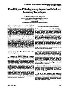
Figure 1. A 30-bin histogram of the proportion of “rock” tags against all other tags.
3.3 Tag prediction with AdaBoost 3.2 Labels as a classification problem Intuitively, automatic labeling would be a regression task where a learner would try to predict tag frequencies for artists or songs. However, because tags are sparse (many artist are not tagged at all) this proves to be too difficult using our current Last.fm / Audioscrobbler dataset. Instead we chose to treat the task as a classification one. Specifically, for each tag we try to predict if a particular artist has “none”, “some” or “a lot” of a particular tag relative to other tags. Note that we use a relative measure. That is, our tags for a given artist are normalized so that artists having many tags can be compared to artists having few tags. Then for each tag, an artist was decided as being “none”, “some” or “a lot” depending on the proportion of times a particular tag was assigned to that artist relative to other tags assigned to that artist. Thus if an artist received only 50 “rock” tags and nothing else, it would be treated as having “a lot” of rock. Conversely, if an artist received 5000 “rock” tags but 10,000 “jazz” tags it would be treated as having “some” “rock” and “a lot” of “jazz”. The specific boundaries between “none”, “some” and “a lot” were decided by summing the normalized tag counts or all artists, generating a 100-bin histogram for each tag and moving the category boundaries such that an equal number of artists fall into each of the categories. In the case of “classical”, the tagging was so sparse that this approach yielded only two bins because there were so many “none” values for “classical” that it was not possible to divide the remaining tagged “classical” examples into two bins of significant size. In Figure 1 the histogram for “rock” is shown (with only 30 bins to make the plot easier to read). Note that most artists are not labeled rock (bin 0) and that otherwise most of the mass is in high-bins. This was the trend for most tags and one of our motivations for using a 3-bin approach.
We now describe how to train an AdaBoost-based classifier to predict the tags based on labeled data. For those interested in more details about how the learning works please see [2], which also used AdaBoost.MH and aggregate features. In short, audio features are extracted from a song. Aggregate features spanning 5 seconds of music are generated. If a song is longer than 5 minutes, only the middle 5 minutes of data are kept (for reasons of computational efficiency). Using MultiBoost.MH a booster is trained to predict the tag (“none”, “some”, “a lot”) directly from the aggregate feature values. The value for a song is taken by voting over the predictions for each aggregate feature. Voting can take place in two ways: we can choose segment winners and then select as global winner the class receiving the most segment votes or we can sum the weak learner values over segments and then take the class with the maximum sum. 3.4 AdaBoost and AdaBoost.MH AdaBoost [4] is a meta-learning method that constructs a strong classifier from a set of simpler classifiers, called weak learners in an iterative way. Originally intended for binary classification, there exist several ways to extend it to multiclass classification. We use AdaBoost.MH [11] which treats multiclass classification as a set of oneversus-all binary classification problems. In each iteration t, the algorithm selects the best classifier, called h(t) from a pool of weak learners, based on its performance on the training set, and assigns it a coefficient α(t) . The input of the weak learner is a d-dimensional observation vector x ∈