Auxiliary Particle Filter Robot Localization from High ... - CiteSeerX

Auxiliary Particle Filter Robot Localization from High-Dimensional Sensor Observations Nikos Vlassis

Bas Terwijn

Ben Kr¨ose

RWCP, Autonomous Learning Functions SNN, Informatics Institute University of Amsterdam, Kruislaan 403, 1098 SJ Amsterdam, The Netherlands 1

Abstract We apply the auxiliary particle filter algorithm of Pitt and Shephard (1999) to the problem of robot localization. To deal with the high-dimensional sensor observations (images) and an unknown observation model, we propose the use of an inverted nonparametric observation model computed by nearest neighbor conditional density estimation. We show that the proposed model can lead to a fully adapted optimal filter, and is able to successfully handle image occlusion and robot kidnap. The proposed algorithm is very simple to implement and exhibits a high degree of robustness in practice. We report experiments involving robot localization from omnidirectional vision in an indoor environment. 1 Introduction In mobile robotics, a topic that has received considerable attention is that of robot localization, a term that refers to the ability of a robot to predict and maintain its position and orientation within its environment. From a statistical point of view, robot localization is an on-line filtering problem: estimate the current state of the robot, given an initial state estimate and a sequence of observations. Many existing approaches rely on Kalman filters for robot state estimation [1]. Although the Kalman filter constitutes a powerful framework, its applicability is restricted by the assumption that the state vector is Gaussian distributed. A popular algorithm which is able to deal with nonGaussian distributions is the particle filter (see [2] for a review). The distribution of the state vector is represented as a set of ‘particles’ in state space. After a novel observation, this set of particles is updated by sampling techniques, using an observation model which describes the likelihood of an observation given the robot state. The filter has been successfully used in robotics (see [3] and references therein). However some of its problems, in particular those related to optimal sampling from the distribution, choice of an observation model, outlier handling, and efficiency of implementation, still remain. 1 http://www.science.uva.nl/research/ias/

For efficient sampling, the auxiliary particle filter of Pitt and Shephard [4] provides an elegant solution when the observation model is known. However, when the latter is unavailable, nonparametric density estimation methods must be employed. In this paper we discuss some traditional ways for doing this and then propose a computationally attractive method that is based on nearest neighbor conditional density estimation [5]. We show how the auxiliary particle filter, which has a built-in capacity to properly handle outliers, can be fully adapted to the proposed observation model, leading to an optimal filter. The proposed algorithm is very simple to implement and exhibits a high degree of robustness in practice, as it can handle aberrant situations like outliers or robot ‘kidnap’. We demonstrate it on a Nomad scout robot equipped with omnidirectional vision, localizing itself in a realistic environment involving large amounts of image occlusion and kidnapping. 2 The robot localization problem A convenient way to analyze the robot localization problem is through a state-space approach.1 The robot is regarded as a partially observable Markov decision process with hidden low-dimensional state xt ∈ X ⊂ IRq that corresponds to position and orientation of the robot (or other parameters of interest) for each time step t. We assume an initial distribution p(x0 ) at time t = 0, and a given stochastic transition model p(xt+1 |xt , ut ) for an action (control signal) ut that is issued at time t and brings the robot stochastically from state xt to state xt+1 . In the following, we will always assume the existence of an action ut in the transition model and for simplicity write p(xt+1 |xt ).

Moreover, we assume that in each time step t the robot observes a high-dimensional sensor vector yt ∈ Y ⊂ IRd , which is related to the robot state through a (possibly unknown) stochastic observation model p(yt |xt ). We assume that the observations {yt } are conditionally independent given the states {xt }, and that d À q. Robot localization, or filtering, amounts to estimating in each 1 Throughout, x will denote both a random vector and its realt ization, and p(xt ) its probability density function at time t.

time step t a posterior density p(xt |yt ) over the state space X , that characterizes the belief of the robot about its current state at time t given its initial belief p(x0 ) and the sequence of observations y1 , . . . , yt . Using the Bayes rule, this posterior density for time t + 1 reads to proportionality p(xt+1 |yt+1 ) ∝ p(yt+1 |xt+1 ) p(xt+1 )

(1)

where the prior density p(xt+1 ) corresponds to the propagated posterior from the previous time step Z p(xt+1 ) = p(xt+1 |xt ) p(xt |yt ) dxt (2) where we used the Markov assumption that the past has no effect beyond the previous time step. The above two formulas constitute an efficient iterative scheme for optimal (Bayesian) filtering. However, in order to compute the posterior (1) analytically, we must be able to compute the integral in (2), then multiply with the likelihood p(yt+1 |xt+1 ), and finally normalize the resulting density p(xt+1 |yt+1 ) to unit integral. It turns out that, unless the transition and observation models are linear-Gaussian (Kalman filter solutions), the above posterior cannot be analytically computed, and one has to resort to approximations or simulation.

Assuming a set of particles that approximate the posterior density p(xt |yt ) at time t sufficiently good, the problem is how to sample a set of particles from the new posterior p(xt+1 |yt+1 ) in (5). Efficiently sampling from the posterior is the central theme of most methods in the particle filters literature [2]. A key observation on the functionality of the filter is that the prior (4) can be regarded as a mixture density from which sampling is easy: select the i-th mixture component p(xt+1 |xit ) with probability πti , and then draw a sample from it.2 The frequently used Sampling/Importance Resampling (SIR) [6, 7, 8] involves first sampling from the above mixture prior, then assigning to each samj pled particle j weight πt+1 proportional to the likelihood p(yt+1 |xjt+1 ), and finally resampling in order to make all particle weights equal.

o − particles l − auxiliary particles

likelihood p(y|x)

prior p(x)

3 The particle filter The particle filter is an attractive simulation-based approach to the problem of computing intractable posterior distributions in Bayesian filtering [2]. The idea is to approximate the continuous posterior density p(xt |yt ) in each time step t by a random sample of i = 1, . . . , I particles xit with corresponding probability masses, or weights, πti . The posterior is then given by the empirical estimate p(xt |yt ) =

I X i=1

πti δ(xt − xit )

(3)

where δ(xt − xit ) is a delta function centered on the particle xit . Using (3), the integration for computing the prior in (2) is now replaced by the much easier summation p(xt+1 ) =

I X i=1

πti p(xt+1 |xit )

(4)

while, since all integrals are replaced by sums and the continuous densities by discrete ones, the required normalization step of the filtered posterior p(xt+1 |yt+1 ) ∝ p(yt+1 |xt+1 )

I X i=1

πti p(xt+1 |xit )

(5)

is trivial, namely, a normalization of the discrete masses to unit sum.

o

o o ooooo o o o llllllllllllllll o

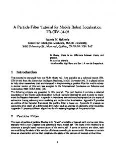
Figure 1: Sampling only from the prior fails to produce enough particles in the overlapping region between the prior and the likelihood function. This is exactly the region where the posterior is nontrivial.

The main problem with the standard SIR particle filter is that it requires very many particles to converge when the likelihood function p(y|x) is too peaked or is situated in one of the prior’s tails [4] (see Fig. 1). The latter is much more severe in case of outliers, model-implausible observations that occur when there is image occlusion or other unexpected effects in the environment. A second important problem in practice is that the observation model p(yt |xt ) may involve high-dimensional vectors yt (e.g., images) and it is in most cases unavailable. 2 Typically the transition model p(x t+1 |xt ) is assumed known and easy to sample from. In the robot application it is often Gaussian, with mean computed from the translation-rotation of the robot, and standard deviation given by the odometry noise characteristics. Sampling from this model is trivial.

4 The auxiliary particle filter An elegant solution to the problem of optimally sampling from the posterior has been given by Pitt and Shephard [4] under the name ‘auxiliary particle filter’. Their algorithm comes down to the following: in order to sample from the posterior p(xt+1 |yt+1 ) in (5), just insert the likelihood inside the mixture p(xt+1 |yt+1 ) ∝

I X i=1

πti p(yt+1 |xt+1 ) p(xt+1 |xit )

(6)

and treat the products πti p(yt+1 |xt+1 ) as component probabilities in order to sample from the respective mixture. Because the likelihood p(yt+1 |xt+1 ) in the above product involves the unobserved state vector xt+1 , an approximation of the mixture (6) has been suggested in [4] as pˆ(xt+1 |yt+1 ) ∝

I X i=1

πti p(yt+1 |µit+1 ) p(xt+1 |xit )

j πt+1 ∝

(8)

i

j where µt+1 is the associated likely value of the mixture i component p(xt+1 |xtj ) in (7) from which the particle j was sampled. Setting the weights of the particles as in (8) has the additional benefit of creating particles with much less variable weights than for the original SIR method, a very important issue especially in the case of outliers [4].

The auxiliary particle filter can be regarded as a onestep look-ahead procedure, where a particle xit is propagated to µit+1 in the next time step in order to assist the sampling from the posterior. The resulting method is particularly efficient since it requires only the ability to sample from the transition model and evaluate the likelihood function p(yt |xt ). This makes it very attractive compared to alternative methods that require specialized data structures for sampling from the posterior. 5 Nonparametric observation models The auxiliary particle filter provides an attractive solution to the problem of efficient sampling from the posterior, and moreover it can handle outliers in a principled manner, however in many practical cases the observation 3 In

5.1 Kernel smoothing When the observation model p(y|x) in the particle filter is unavailable, one possibility—hinted in [4, Sec. 7]— is to estimate it nonparametrically, that is, using a supervised training set of robot states {xk } and respective observations {yk }, for k = 1, . . . , K. A classical method is through kernel smoothing [9], an approach we have used in the past for similar modeling problems [10]. This method places multivariate kernels on each stateobservation pair, and then estimates the unknown conditional density by

(7)

where µit+1 is any likely value associated with the i-th component transition density p(xt+1 |xit ), for example its mean.3 After a set of j = 1, . . . , I particles have been sampled4 from the mixture (7), with locations xjt+1 , their weights are set proportional to p(yt+1 |xjt+1 ) ij p(yt+1 |µt+1 )

model p(y|x) required by the filter is unavailable. The estimation of a good model for p(y|x) from data is often a difficult task, especially when the sensor observations y of the robot are very high-dimensional (e.g., image data). In the following we first describe a ‘classical’ method for estimating conditional densities from a set of data, and then propose our model.

our model, such an approximation can be replaced by an exact step, as we show in Section 6. 4 This involves a multinomial sampling on the weights, and there is an O(I) procedure for doing this [4].

p(y, x) = p(y|x) = p(x)

PK

φ(x|xk ) ψ(y|yk ) PK k=1 φ(x|xk )

k=1

(9)

where φ(x|xk ) and ψ(y|yk ) are appropriate density kernels in the X and Y spaces, respectively. However, the high dimensionality of the observations y causes each neighborhood of interest in the Y space to look sparse of data, the notorious ‘curse of dimensionality’. To adequately model p(y|x) through (9) one would need a kernel ψ(y|yk ) with very large bandwidth (standard deviation in case of a Gaussian kernel), smoothing away any useful information in the training data. This fact renders the direct application of kernel smoothing in the Y space impossible.

One solution would be to project first the data {yk } to a subspace of lower dimension, for example by using principal component analysis (PCA) or some other feature extraction method [11, 12]. However, kernel smoothing is known to work effectively only in low dimensions (e.g., up to five), implying that we would need a compression of the Y space that would throw away valuable location discrimination information: the resulting data manifold in the feature space would exhibit self-intersections that would enter the localization algorithm as perceptual aliasing [12].

Moreover, kernel smoothing is slow, with cost O(K): for each evaluation of the observation model (9), a complete summation over the training data is required, making the method inefficient for practical applications. 5.2 A nearest neighbor-based model The above limitations of kernel smoothing motivate a different approach to deal with high-dimensional sensor observations. First, we linearly project the training observations with PCA to a subspace of moderately low dimen-

sion, e.g., 10-D.5 Then, instead of modeling the density p(y|x), we ‘invert’ it using the Bayes rule p(y|x) =

f (x|y)f (y) f (x)

(10)

and then model the density f (x|y) nonparametrically using nearest neighbor conditional density estimation [5]. This is feasible because the dimensionality of the state space is low (e.g., q = 3, if the state combines position and orientation of a robot on the plane). The robot states {xk } in the training set are assumed uniformly sampled over the state space and therefore the denominator in the above formula can be assumed constant and thus can be dropped. For the conditional density f (x|y) the proposed model reads f (x|y) =

J X

mechanism is a simple threshold test of the distance of an observation y to its first nearest neighbor yj=1 , with the threshold parameter computed by collecting statistics of all pairwise distances between the training observations (a detailed description is omitted due to lack of space). If occlusion is detected, the auxiliary particle filter sampling is not used and the filter just propagates the particles from the previous time step according to the transition model. The whole procedure has time complexity O(J log K) which is a significant improvement O(K) cost of kernel smoothing (typically J and moreover it can be successfully applied dimensional observations.8

at most over the ¿ K), to high-

6 Filter adaption λj (y) φ(x|xj ),

(11)

j=1

i.e., a mixture of J components φ(x|xj ), each weighted by λj (y), which is computed as follows: 1. We first find the J nearest neighbors yj of y among the {yk } training data. This can be done efficiently—with average cost O(J log K)—using methods from computational geometry, e.g., kdtrees [13]. 2. We sort these neighbors yj by increasing distance to y, so j = 1 for the nearest, j = 2 for the second nearest, and so on. This costs O(J log J). 3. For each nearest neighbor yj we extract from the training set the corresponding state xj . This has cost O(J). 4. Each xj defines a respective component φ(x|xj ) in the mixture (11). The function φ(x|xj ) is a Gaussian kernel centered on xj with bandwidth equal to half the bin size of the grid of the {xk } points. 5. Finally, the mixing weights λj (y) are positive and sum to one, and decrease linearly with j λj (y) =

2(J − j + 1) . J(J + 1)

(12)

Note that they are independent of the actual distance of y to its neighbors j.6 Finally, the density f (y) in (10) is considered only against the presence of outliers (e.g., occlusion in the image), but otherwise is assumed uniform.7 The outlier detection 5 The choice of projection dimension is guided by the dimensionality of X , but space precludes further discussion. 6 More sophisticated weights can also be defined, see [5]. 7 Note that, for large dimensions, it is difficult to make reasonable assumptions about the true shape of f (y) using reasonably sized training sets. The theoretically crude assumption of uniform f (y) has, in practice, no serious consequences.

We show here that the proposed choice of nonparametric model for the observation density, through nearest neighbor conditional density estimation, can lead to a fully adapted particle filter. The term refers to the case where we can exploit the structure of the problem and sample exactly (without approximation) from the unknown posterior [4]. Assuming uniform f (x) and f (y) in (10), and the proposed model of f (x|y) as in (11), the posterior p(xt+1 |yt+1 ) in (6) reads to proportionality ∝

I X

=

I X J X

i=1

πti

p(xt+1 |xit )

i=1 j=1

J X j=1

λj (yt+1 ) φ(xt+1 |xj )

πti λj (yt+1 ) p(xt+1 |xit ) φ(xt+1 |xj ).

(13)

From the last equation we see that the posterior can be written as a mixture of I × J components, with each component being a product of the transition density p(xt+1 |xit ) and the local Gaussian kernel φ(xt+1 |xj ). In the common case of a Gaussian transition density, this product can be written in terms of a Gaussian density over xt+1 and another quantity which is not a function of xt+1 . For example, in the simple case of a twodimensional state space and equal odometry noise standard deviation and bandwidth of φ(·), say σ, straightforward algebra shows that the product reads p(xt+1 |xit ) φ(xt+1 |xj ) = g(xt+1 |xit , xj , σ) h(xit , xj , σ) (14) where g(xt+1 |xit , xj , σ) is a bivariate Gaussian with mean √ (xit + xj )/2 and standard deviation σ/ 2, and h(xit , xj , σ) =

¶ µ 1 ||xit − xj ||2 . exp − 4πσ 2 2σ 2

(15)

8 One should note, however, that the cost of finding nearest neighbors typically increases with the dimension [13].

The posterior p(xt+1 |yt+1 ) in (13) becomes then proportional to J I X X i=1 j=1

πti λj (yt+1 ) h(xit , xj , σ) g(xt+1 |xit , xj , σ) (16)

from which sampling is easy: first select the ‘joint component’ (i, j) with probability proportional to πti λj (yt+1 ) h(xit , xj , σ), and then sample from the corresponding Gaussian g(xt+1 |xit , xj , σ). The time complexity of this operation is O(IJ) (the cost of multinomial sampling in the joint space), but typically J ¿ I, (in our experiments J = 5), while the filter works satisfactorily even with a small number of particles (we used I = 200). The above procedure obviates the need for an approximate look-ahead procedure as in (7), leading to an optimal, fully adapted filter. The complete algorithm has time complexity O(J log K + IJ), i.e., it scales linearly with the number of particles and logarithmically with the number of training data. 7 Robot kidnap

A

B

C

Figure 2: The path of the robot in our building. 100 using odometry using vision+PF 90

80

70

localization error

∝

60

50

40

30

Robot kidnap refers to the case where the robot is lifted and manually repositioned in a different location in the environment, and has to relocalize itself based on the new sensor evidence. While outliers refer to modelimplausible observations under model-plausible motion, kidnap can be regarded as the dual, model-implausible motion with model-plausible observations. To handle this case we have followed a standard approach in the literature [14, 15]: first detect the discrepancy between the prior and the observation likelihood, and then sample a subset of particles directly from the likelihood. However, a more careful treatment is needed in very degenerate cases, for example when a persistent outlier ‘looks like’ kidnap, or if we allow both motion and observation models to be violated (combined kidnap and outliers). We are currently developing a method for handling these degenerate cases by explicitly taking the ‘age’ of a particle into account—i.e., how long the particle has survived the sampling process—when sampling from the various distributions. Details of this method will be reported elsewhere.9 8 Experiments We illustrate the performance of the algorithm applied on our Nomad Scout robot equipped with an omnidirectional vision system. First we captured 33 panoramic images by positioning the robot on a grid of locations in the laboratory, corridor, and hall of our building (Fig. 2), while the orientation of the robot was registered at these locations. The distance between the locations was about 50 cm. For each position we created images the robot would see at 9 See

also http://www.science.uva.nl/~bterwijn

20

10

0

1

2

3

4

5 6 number of path traversals

7

8

9

10

Figure 3: The localization error of the robot using odometry only and using the particle filter for a number of path traversals.

36 orientations by shifting the original panorama image, thus creating a database of approximately 1000 images. From these images we took a subset of 300 images to compute the PCA projection. The first 10 components of the PCA were used to project all training images to 10-D feature vectors. The environment representation finally consisted of 1000 10-D vectors. The robot was programmed to follow the path shown in Fig. 2 starting in the laboratory (point A), going through the door to the corridor (point B), reaching the hall (point C), and then coming back to the laboratory, for a number of times. In Fig. 3 we plot the localization error of the robot (in cm, the robot orientation is ignored) for a number of path traversals when using only odometry and when using our particle filter algorithm. After eight traversals, by using only odometry the robot is almost one meter far off its true location. In a second experiment we investigated the capability of the algorithm to recover from kidnap situations. The robot was programmed again to follow the path from A to C, but at point K we kidnapped the robot as shown in Fig. 4-5. We lifted the robot manually and repositioning it at the same location with a rotation of 180 degrees.

Sequential Monte Carlo Methods in Practice, SpringerVerlag, 2001. [3] S. Thrun, D. Fox, W. Burgard, and F. Dellaert, “Robust Monte Carlo localization for mobile robots,” Artificial Intelligence, vol. 128, no. 1-2, pp. 99–141, May 2001. [4] M. K. Pitt and N. Shephard, “Filtering via simulation: Auxiliary particle filters,” J. Amer. Statist. Assoc., vol. 94, no. 446, pp. 590–599, June 1999.

Figure 4: The kidnap!

[5] C. J. Stone, “Consistent nonparametric regression (with discussion),” Ann. Statist., vol. 5, pp. 595–645, 1977.

450 PF estimate odometry estimate

A

400

[6] N. J. Gordon, D. J. Salmond, and A.F.M. Smith, “Novel-approach to nonlinear non-Gaussian Bayesian state estimation,” IEE Proceedings-F Radar and signal processing, vol. 140, no. 2, pp. 107–113, 1993.

350

y coordinate (in cm)

300

K

250

[7] M. Isard and A. Blake, “Condensation - conditional density propagation for visual tracking,” Int. J. Comp. Vision, vol. 29, no. 1, pp. 5–28, 1998.

200

B

C

150

100

50

0 −300

−200

−100

0

100 200 x coordinate (in cm)

300

400

500

Figure 5: The trajectory of the robot from A to C with a kidnap at point K.

The robot was able to recover and, after some exploration around K, could find its way back to the planned destination point C. We have also successfully demonstrated our localization method in the three-day final exhibition of the Real World Computing Project [16]. For more than 30 hours of operation, our robot was able to track its correct position and orientation, and recover from unexpected situations, for example when people were occluding the scene or the robot was kidnapped for demonstration purposes. Our algorithm exhibited a particularly robust behavior in this realistic experiment involving large amounts of noise and dynamic real-world characteristics. Acknowledgments Many thanks to Roland Bunschoten and Edwin Steffens for contributing to this work in various ways. This research has been supported by the Real World Computing Partnership. References [1] S. I. Roumeliotis and G. A. Bekey, “Bayesian estimation and Kalman filtering: A unified framework for mobile robot localization,” in Proc. IEEE Int. Conf. on Robotics and Automation, San Fransisco, CA, Apr. 2000, pp. 2985–2992. [2]

A. Doucet, N. de Freitas, and N. Gordon, Eds.,

[8] F. Dellaert, D. Fox, W. Burgard, and S. Thrun, “Monte carlo localization for mobile robots,” in Proc. IEEE Int. Conf. on Robotics and Automation, Detroit, Michigan, May 1999. [9] M. P. Wand and M. C. Jones, Kernel Smoothing, Chapman & Hall, London, 1995. [10] B.J.A. Kr¨ose, N. Vlassis, R. Bunschoten, and Y. Motomura, “A probabilistic model for appearancebased robot localization,” Image and Vision Computing, vol. 19, no. 6, pp. 381–391, Apr. 2001. [11] N. Vlassis, Y. Motomura, and B. Kr¨ose, “Supervised linear feature extraction for mobile robot localization,” in Proc. IEEE Int. Conf. on Robotics and Automation, San Fransisco, CA, Apr. 2000, pp. 2979–2984. [12] N. Vlassis, Y. Motomura, and B. Kr¨ose, “Supervised dimension reduction of intrinsically low-dimensional data,” Neural Computation, vol. 14, no. 1, pp. 191–215, Jan. 2002. [13] M. de Berg, M. van Kreveld, M. Overmars, and O. Schwarzkopf, Computational Geometry: Algorithms and Applications, Springer-Verlag, Berlin, 1997. [14] P. Jensfelt, D. J. Austin, O. Wijk, and M. Andersson, “Experiments on augmenting condensation for mobile robot localization,” in Proc. IEEE Int. Conf. on Robotics and Automation, San Fransisco, CA, Apr. 2000, pp. 2518–2524. [15] S. Lenser and M. Veloso, “Sensor resetting localization for poorly modelled mobile robots,” in Proc. IEEE Int. Conf. on Robotics and Automation, San Fransisco, CA, Apr. 2000, pp. 1225–1232. [16] Real World Computing Partnership, “Final exhibition & symposia,” Tokyo Fashion Town, Japan, organized by the National Institute of Advanced Industrial Science and Technology of Japan (AIST), Oct. 2001, http://www.rwcp.or.jp/rwc2001.