All Atheros chipset extensions are disabled. The experiments were conducted outdoor on 802.11a channel 36. The throughput of an isolated link is around.
This full text paper was peer reviewed at the direction of IEEE Communications Society subject matter experts for publication in the IEEE ICC 2009 proceedings
Back-of-the-Envelope Computation of Throughput Distributions in CSMA Wireless Networks Soung Chang Liew, Caihong Kai The Chinese University of Hong Kong Hong Kong SAR, P.R.China {soung, chkai6}@ie.cuhk.edu.hk Abstract— This paper presents a simple method for computing throughputs of links in a CSMA network. We call our method back-of-the-envelop (BoE) computation, because for many network configurations, very accurate results can be obtained by simple hand computation. BoE beats prior methods in terms of both speed and accuracy. To explain BoE, we construct a theory based on the model of an “ideal CSMA network” (ICN). We find that link throughputs are insensitive to the distributions of the backoff countdown time and transmission time in ICN given the ratio of their mean c. The BoE computation method emerges from ICN in the limit c → 0 . The insensitivity result explains why BoE works so well for IEEE 802.11 networks, in which the backoff countdown process is one that has memory and the transmission time can be arbitrarily distributed. Furthermore, c does not have to be very small for BoE to be highly accurate. BoE allows us to make shortcuts in performance evaluation, bypassing complicated stochastic analysis. An immediate application of BoE is for quick identification of starved links in the network so that remedies can be devised to solve the problem. Index Terms—CSMA, 802.11, Wi-Fi, multiple access.
Jason Leung, Bill Wong Altai Technologies Hong Kong SAR, P.R. China {hcleung, billwong}@altaitechnologies.com if it senses the transmission of another link within its carrier-sensing range (CSRange). The carrier-sensing relationship is described by the contention graph on the right, in which links are represented by vertices, and an edge joins two vertices if the transmitters of the two associated links can sense each other. The “normalized” throughputs of the links (Th1 Th2 Th3 Th4 ) can be quickly approximated to be (1 0 0.5 0.5) within seconds, as described below. With respect to the contention graph, we try to put a label of 1 to as many vertices as possible with the constraint that two vertices joined by an edge cannot both be 1 (i.e., 1 represents transmission, and two links that can sense each other cannot transmit together). We have two possible configurations: (1 0 1 0) and (1 0 0 1). We add the vectors together and divide the sum by 2, yielding (1 0 0.5 0.5) . And these are the normalized link throughputs (Th1 Th2 Th3 Th4 ) . The procedure is purely algorithmic, and there is no complex stochastic analysis.
I. INTRODUCTION With the widespread deployment of IEEE 802.11 networks, it is now common to find multiple wireless LANs co-located in the neighborhood of each other. The carrier-sensing relationships among the links of these networks are non-all-inclusive in that each link may only sense a subset, but not all, of other links. It is very difficult to extend the analytical methods for the all-inclusive case (e.g., [1]), where all links can sense all other links, to the non-all-inclusive case. Given its practical relevance, good approximation techniques for estimating link throughputs in the non-all-inclusive case are highly desirable. This paper presents one such method. We refer to it as a back-of-the-envelop (BoE) computation method because for networks of modest size, the results can be obtained in a matter of minutes, if not seconds, with simple hand computation. In particular, complicated stochastic analysis is not necessary. BoE allows us to make shortcuts in system performance evaluation. A practical application of BoE is for quick identification of problems in a network (e.g., unfair throughput distributions and starvation) so that remedies could be devised to solve them. To illustrate its simplicity, let us first describe the mechanics of BoE without justification. Consider the network on the left of Fig. 1. In this network, a link will not initiate a transmission This work was partially supported by the Competitive Earmarked Research Grant (Project Number 414507) established under the University Grant Committee of the Hong Kong Special Administrative Region, China.
Figure1. An example network and its associated contention graph.
We were originally led to the BoE algorithm from observation of simulation and real-network experimental results rather than from theoretical construction. In this paper, we attempt to explain BoE with an ideal CSMA network model (ICN). BoE emerges from ICN when the ratio of the mean backoff countdown time and mean transmission time of the CSMA protocol, c, approaches zero. We find that 1) the link throughputs in ICN are insensitive to the distributions of the backoff countdown time and transmission time given c; and 2) c does not have to be very small for BoE to be accurate. These results explain why the throughputs computed by BoE match so well with NS2 simulation results of 802.11 networks. Related Work There have been many publications on non-all-inclusive CSMA networks. Recent work includes [2–7], from which earlier work can be traced. Most of the prior methods are stochastic-analytical and not algorithmic in nature. BoE in this
978-1-4244-3435-0/09/$25.00 ©2009 IEEE Authorized licensed use limited to: Chinese University of Hong Kong. Downloaded on August 26, 2009 at 23:10 from IEEE Xplore. Restrictions apply.
This full text paper was peer reviewed at the direction of IEEE Communications Society subject matter experts for publication in the IEEE ICC 2009 proceedings
paper is algorithmic and is simpler. As far as we know, the CSMA network model with exponential idle and transmission times was first considered in [8]. More recent work that models the backoff and transmission processes with exponential distributions includes [9, 10]. The assumption of exponential backoff time, however, is not compatible with practical CSMA protocols (e.g., 802.11), in which the backoff process has memory. Typically, the backoff process is controlled by a counter. When the counter is decremented to zero, then transmission begins. The countdown freezes whenever a neighbor starts to transmit. When the transmission of the neighbor completes, the countdown resumes with the previous counter value when the link was last frozen. The general ICN model in this paper takes this feature into account. A contribution of ours is the proof that the link throughputs in ICN are insensitive to this memory effect and to the distributions of the backoff countdown and transmission times given the ratio of their means c. This expands the scope of the application of BoE and ICN. Our technical report [11] contains interesting results not presented here. For example, in [11] we show that the system-state probability distribution of ICN is a Markov random field [12]. Three proofs of our aforementioned insensitivity results providing different perspectives and insights can also be found in our technical report. II.
Thsingle link = 6.06Mbps (for 11Mbps 802.11b) 25.38 Mbps (for 54 Mbps 802.11g) 29.45Mbps (for 54 Mbps 802.11a) The actual throughput of a link with a normalized throughput of Thnorm is then computed as Thactual = Thnorm ⋅ Thsingle link . Fig. 2 shows the results of BoE computation for various network topologies, and the corresponding NS2 simulations results for UDP and TCP sessions. Typical 802.11b and default NS2 parameters were used in the simulations: (i) data rate and basic rate of 11Mbps and 1Mbps, respectively; (ii) carrier-sensing range of 550m; (iii) packet payload of 1460 Bytes for both UDP and TCP; (iv) for each UDP session, a CBR flow of 7Mbps > Thsingle link = 6.06Mbps was used to ensure link saturation; TCP, being greedy in nature, automatically ensures link saturation; after taking into account TCP_ACK, Thsingle link = 4.84Mbps . Finally, the link length was fixed to 5m for all links. Each simulation simulated 200 seconds of network dynamic. As can be seen from Fig. 2, the accuracy of BoE is quite amazing for such a simple method. Simulations of many other topologies also bear out BoE. (1)
BOE COMPUTATION AND EXPERIMENTAL VERIFICATION The following formalizes the description of BoE: BoE Computation Draw the contention graph of the network. Identify the maximum independent sets (MIS) of the contention graph. The normalized throughput of link i is ni n , where n is the number of MIS identified in Step 2, and ni is the number of MIS in which link i appears. Convert normalized throughputs to throughputs in bps.
(3)
An independent set (IS) is a subset of vertices such that no edge joins any two of them; and an MIS is an IS with the maximum cardinality [13]. We note that counting MIS is an NP-complete problem, and therefore BoE can get out of hand for networks of very large size. However, for networks of modest size, such as 802.11 networks within a building, the problem is manageable. Generally, for networks of up to 10 links, hand computation is possible and quick. For random networks of up to 100 links, results can be obtained within a few minutes by a MATLAB program. With the technique of link aggregation (see later part of this section), even larger networks can be dealt with.
(5)
1. 2. 3.
4.
Refer to Fig. 1 again. The MIS identified in Step 2 are (1 0 0 1) and (1 0 1 0). Step 3 determines the normalized throughput distribution to be (1 0 0.5 0.5). In Step 4, a normalized throughput of 1 corresponds to the throughput of a link transmitting in isolation of other links as if it were the only link in the whole network. After taking into account the various headers (see Section III.A), the throughput of an isolated link for a UDP session is typically
(7)
(2)
(0, 1, 1, 1)
BoE
(1, 0, 0,1)
NS2, UDP
(0.96, 0.02, 0.02, 0.97)
(0.03, 0.99, 0.98,1)
NS2, TCP
(0.97, 0.01, 0.01, 0.97)
(0.02, 0.99, 1, 1)
Real network
(0.76, 0.10, 0.10, 0.74)
(0.1, 0.8, 0.8, 0.8)
BoE
(1, 0, 0.5, 0.5)
NS2, UDP
(0.99, 0, 0.50, 0.51)
(0.75, 0.26, 0.26, 0.26, 0.51)
NS2, TCP
(0.99, 0, 0.49, 0.51)
(0.74, 0.25, 0.24, 0.25, 0.50)
BoE
(0.4, 0.4, 0.4, 0.4, 0.4)
NS2, UDP
(0.41, 0.40, 0.41, 0.40, 0.40)
(0.92, 0.04, 0.04, 0.92, 0.04, 0.93)
NS2, TCP
(0.40, 0.39, 0.40, 0.40, 0.40)
(0.95, 0.02, 0.02, 0.95, 0.03, 0.95)
BoE
(0.5, 0.5, 0.5, 0.5, 0.5, 0.5)
NS2, UDP
(0.5, 0.5, 0.49, 0.5, 0.5, 0.5)
(0.20, 0.41, 0.41, 0.80, 0.60, 0.60)
NS2, TCP
(0.46, 0.51, 0.51, 0.46, 0.46, 0.51)
(0.21, 0.39, 0.4, 0.79, 0.61, 0.60)
(4)
(6)
(8)
(0.75, 0.25, 0.25, 0.25, 0.5)
(1, 0, 0, 1, 0, 1)
(0.2, 0.4, 0.4, 0.8, 0.6, 0.6)
Figure 2. Contention graphs of various network topologies and the BoE computed and experimental results for them.
For larger networks, we present results of ten experiments with ten randomly generated 50-link networks. The mean
Authorized licensed use limited to: Chinese University of Hong Kong. Downloaded on August 26, 2009 at 23:10 from IEEE Xplore. Restrictions apply.
This full text paper was peer reviewed at the direction of IEEE Communications Society subject matter experts for publication in the IEEE ICC 2009 proceedings
degree of links (number of neighbors per link) is around 4. For each link, we calculated the error of the throughput computed by BoE relative to the simulated throughput. The error is normalized by the maximum link throughput in the network. The average link throughput error of the ten runs is around 5%. Fig. 3 shows the detailed comparison of one such run, where the normalized throughput of each link is plotted. As can be seen, BoE is a highly accurate estimation method. Additional BoE results will be presented in Section IV. 1.2 BoE Prediction
1.1
Simulation
[(1 0 1 0) × 6 + (1 0 0 1) × 3 + (0 1 0 1)] / 10 = (0.9 0.1 0.6 0.4) . The throughput of an original link is then the throughput of its virtual link divided by the cardinality of the virtual link. In our example, links 1, 2, and 3 have throughput of 0.9 3 = 0.3 ; link 4 has throughput of 0.1; links 5 and 6 have throughput of 0.6 2 = 0.3 ; and link 7 has throughput of 0.4.
1 Normalized throughput
cardinalities of the virtual vertices it contains (e.g., the cardinality of (1 0 1 0), (1 0 0 1), and (0 1 0 1) are 3 ⋅ 2 = 6 , 3 ⋅ 1 = 3 , and 1 ⋅ 1 = 1 , respectively). Note that each virtual MIS can be mapped to one or more original MIS, and the cardinality of a virtual MIS is the number of original MIS it represents. Thus, the total number of MIS, n, in the original contention graph is the sum of the cardinalities of the virtual MIS, which in our example is 6 + 3 + 1 = 10 . The normalized throughput distribution of the virtual links is ∑ k (MISk × Cardinality of MISk ) / n . In our example, we have
0.9 0.8 0.7 0.6 0.5 0.4 0.3 0.2 0.1 0
0
10
20 30 Link index
40
50
Figure 3. Verification of BoE for a random network of 50 links.
Besides simulations, BoE is also borne out by real network experiments. We set up two topologies ((1) and (2) in Fig. 2) with four pairs of DELL Latitude D505 laptops PCs with 1.5GHz Celeron Mobile CPU. Each node has a NETGEAR WAG511GE Dual Band Wireless PC card, and run Fedora5 with MADWifi [14] driver. All Atheros chipset extensions are disabled. The experiments were conducted outdoor on 802.11a channel 36. The throughput of an isolated link is around 29Mbps. As shown in Fig. 2, the experiment results match well with BoE’s prediction. In the real environment, we found it difficult to totally isolate two links to keep them out of carrier-sensing range. This is the reason why the measured throughput distributions are not as extreme as predicted. BoE with Link Aggregation These days, inside a building there are typically many 802.11 WLANs with many APs. Consider the links associated with any one of the APs. It is likely for some of these links to form a clique and that they have the same carrier-sensing relationships with other links. In infrastructure WLAN deployments, the technique of link aggregation can be very useful for complexity reduction, allowing BoE to handle much larger networks than otherwise possible. We describe the mechanics of BoE with link aggregation in the next paragraph, with the aid of the example in Fig. 4. We omit detailed justification here: that the procedure will yield similar results as the original BoE is self-evident after a little thought. In Fig. 4, the contention graph in (a) becomes the “virtual” contention graph in (b) after link aggregation. The virtual contention graph is a linear graph with four virtual vertices {1,2,3}, {4}, {5,6}, {7}. The virtual MIS for the virtual contention graph are (1 0 1 0), (1 0 0 1), and (0 1 0 1). Let us define the cardinality of a virtual vertex as the number of original links it contains (e.g., the cardinality of {1,2,3} is 3); and the cardinality of a virtual MIS as the product of the
Figure 4. Illustration of link aggregation where the contention graph in (a) is simplified to the contention graph in (b).
III.
EXPLAINING BOE USING ICN
We were originally led to BoE from observation of simulation and real-network experimental results rather than from analytical construction. The structural simplicity of BoE led us to believe that there might be a deeper underlying theory. In this section, we attempt to explain why BoE works in terms of an ideal CSMA network model (ICN). Not long after BoE was discovered from experimental observations, we quickly realized two essential underpinnings of Steps 1 to 3 (see Section II), as embodied in the following propositions: Proposition 1: The system spends most of its time in MIS, and very little time in other states. Proposition 2: The MIS states are equally likely. That is, the system spends approximately equal amounts of time in each MIS. Step 2 of BoE makes the rough approximation that the system spends zero time in non-MIS. Step 3 of BoE implicitly makes use of Proposition 2. We will show that Proposition 2 is implied by ICN, and that Proposition 1 is obtained in the limit of c → 0 in ICN. Before we begin, let us briefly review the 802.11 CSMA protocol [15] to relate the various parameters in 802.11 to the BoE and ICN models. A. Quick Review of 802.11 CSMA Protocol In 802.11, a station that has packets to send must first sense the channel to be idle for duration of DIFS (Distributed Interframe Spacing) plus a random number of backoff timeslots before transmitting a packet. For each new
Authorized licensed use limited to: Chinese University of Hong Kong. Downloaded on August 26, 2009 at 23:10 from IEEE Xplore. Restrictions apply.
This full text paper was peer reviewed at the direction of IEEE Communications Society subject matter experts for publication in the IEEE ICC 2009 proceedings
transmission attempt, the station chooses a random integer backoff counter value uniformly distributed in the range of [0, CW], where CW is referred to as the contention window. For a new packet with no prior collisions, CW is initially set to CWmin. The backoff counter is decremented by one for each slot the channel is sensed idle. If the channel is sensed busy before the counter reaches zero, the countdown is frozen until the channel is sensed idle for a DIFS period again, whereupon the countdown continues with the previous counter value. After transmitting a packet, the sender expects to receive an acknowledgement (ACK) after a SIFS (Short Inter Frame Spacing) period. For an isolated link, the time consumed by a successful packet transmission consists of (i) PACKET duration consisting of physical-layer preamble/header, MAC Header, and data payload; (ii) SIFS; (iii) ACK; (iv) DIFS; (v) the random number of backoff countdown timeslots. For each packet, the airtime within its carrier-sensing range that must be exclusively dedicated to it is Ttr = PACKET + SIFS + ACK+DIFS
(1)
In addition, it also consumes a random backoff countdown time of Tcd (i.e., component (v) above). In this paper, we define the countdown overhead as c = E[Tcd ] / E[Ttr ] (2) When collisions are rare, E[Tcd ] ≈ Tslot × CWmin / 2 . Note that Tcd is the “active” countdown time of a link and that frozen time due to a neighbor’s transmission is not included in it. Thus, c does not include the freezing overhead. Henceforth in this paper, Ttr will be referred to as the transmission time, and Tcd will be referred to as the countdown time. B.
Definition of ICN
Definition of ICN: In ICN, the countdown times of links are continuous random variables. The distributions of countdown time Tcd and transmission time Ttr can be arbitrary otherwise. When a link completes a transmission, it begins countdown with Tcd generated according to the probability density f (tcd ) . When the countdown completes, the link begins to transmit with Ttr generated according to the probability density g (ttr ) . The countdown of a link is frozen whenever at least one of its neighbors transmits, and the remaining countdown time RC will be stored; when all neighbors stop transmitting, the countdown will resume with , the previously stored RC .
Let Si ∈ {0,1} denote the state of link i, where Si = 1 if link i is transmitting and Si = 0 if link i is not transmitting. When link i is not transmitting, it is either actively counting down or frozen. We can define the system state of an ICN with L links as S = S1 S 2 ... S L , where the feasible states correspond to the independent sets of the contention graph of the network. Note that if links i and j are neighbors, then the states in which Si and S j are both 1 are not allowed because (i)
they can sense each other; and (ii) the probability of them counting down to zero and transmitting together is 0 under ICN (because the countdown time is a continuous random variable). Fig. 5 shows the state-transition diagram of the network in Fig. 1 under the ICN model. To avoid clutters, in Fig. 5 we have merged the two directional transitions between two states into one line. Each transition from left to right corresponds to the beginning of a transmission on one particular link, while the reverse transition corresponds to the ending of a transmission on the same link. For example, the transition from 1000 to 1010 is due to the beginning of a transmission on link 3 while link 1 is transmitting; while the reverse transition from 1010 to 1000 is due to the ending of a transmission on link 3 while the transmission of link 1 continues. 1000 0100 0000 0010
1010
0001
1001
Fig. 5. The state-transition diagram of the network in Fig. 1 under ICN model.
C. ICN with Memoryless Exponentially-Distributed Backoff and Transmission Times
According to the definition of ICN, the distributions of Tcd and Ttr can be arbitrary. To simplify exposition, however, we first assume that their distributions are exponential. Definition of State Connectivity: Two feasible state realizations S = s and S = s ' are said to be connected if it is possible to have a direct transition from s to s ' , and vice versa, without traversing other states. For example, in Fig. 5, 1000 and 1010 are connected; but 1010 and 1001 are not connected. Observation 1: Two feasible states s and s ' are connected if and only if all the links transmitting in s are also transmitting in s ' , and there is one extra link transmitting in s ' that is not transmitting in s ; or vice versa. Definition of Left and Right States: For two connected states, we refer to the state with one fewer (more) link transmitting as the left (right) state. Throughput Computation in ICN Let Ps = Ps1s2 ... sL be the fraction of time the network is in a
particular state s = s1s2 ... sL . Under the exponentialdistribution assumption, S (t ) is a Markov process. The fraction of time link i is transmitting is xi =
∑P
s:si =1
s1 s2 ... sL
,
which corresponds to the normalized throughput of link i. Let 1/ λ = E[Tcd ] and 1/ μ = E[Ttr ] . Then for any pair of connected states, the transition from the left state to the right state occurs at rate λ = 1/ E[Tcd ] , and the transition from the
Authorized licensed use limited to: Chinese University of Hong Kong. Downloaded on August 26, 2009 at 23:10 from IEEE Xplore. Restrictions apply.
This full text paper was peer reviewed at the direction of IEEE Communications Society subject matter experts for publication in the IEEE ICC 2009 proceedings
right state to the left state occurs at rate μ = 1/ E[Ttr ] . It is easy to verify that the resulting continuous-time Markov chain is time-reversible and therefore detailed balance applies [12]. Specifically, for two connected states s and s ' , with s being the left state and s ' being the right state, we have Ps = cPs '
(3)
where c = E[Tcd ] / E[Ttr ] = μ / λ is the countdown overhead defined in (2). An immediate corollary of Observation 1 and (3) is that all feasible states with the same number of transmitting links (i.e., states in the same column of the state-transition diagram) have the same probability. Specifically, let S ( n ) be the subset of feasible states with n transmitting links. Then, Ps =
B cn
⎛ L | S ( n) | ⎞ where B = ⎜ ∑ n ⎟ ⎝ n=0 c ⎠
∀ s ∈ S (n) ,
−1
(4)
Applying (4) to the state-transition diagram of Fig. 5 gives P0000 = B = (1 + 4 / c + 2 / c
)
2 −1
P1000 = P0100 = P0010 = P0001 = ( c + 4 + 2 / c )
−1
(5)
P1010 = P1001 = ( c + 4c + 2 ) The normalized throughputs of the links are then given by −1
2
x1 = P1000 + P1010 + P1001 = ( c + 4 + 2 / c ) + 2 ( c 2 + 4c + 2 ) −1
x2 = P0100 = ( c + 4 + 2 / c )
−1
x3 = P0010 + P1010 = ( c + 4 + 2 / c ) + ( c 2 + 4c + 2 ) −1
x4 = P0001 + P1001 = ( c + 4 + 2 / c ) + ( c 2 + 4c + 2 ) −1
D. Insensitivity Transmission Times
to
−1
Distributions
of
−1
−1
Backoff
(6) and
It turns out that Ps as expressed in (4) is insensitive to the distributions of backoff countdown and transmission times, f (tcd ) and g (ttr ) , given the ratio of their means c. Neither is it sensitive to the fact that the countdown process has memory. This result is important because for practical CSMA protocols (e.g., 802.11) and network applications (e.g., FTP and P2P file download), neither the countdown nor transmission time is exponentially distributed. Due to space limitation, we omit the proof of the insensitivity result here, and refer interested readers to our technical report [11]. E. Mapping ICN Results to BoE Computation Method Steps 1 to 3 of BoE are implied by the ICN results in (4) in the limit that c → 0 . Recall from the beginning of this section that BoE is founded on Propositions 1 and 2. According to (4), in the limit c → 0 , only the MIS (the right-most states in the state-transition diagram) has significant probabilities, and the probabilities of the other IS in ICN become negligible compared with the probabilities of MIS because of the factor 1 / c n . In addition, all the MIS have equal probability. In short, Proposition 1 is obtained when c → 0 , and Proposition 2 is due to the form of the ICN results in (4). Converting Normalized Throughputs to Actual Throughputs
In the final step of BoE (Step 4), we need to convert the normalized throughputs to actual throughputs in bps. This is the engineering part with different alternatives. This paper adopts a very simple procedure. We simply multiply the normalized throughputs by the raw throughput of a single isolated link to obtain the throughputs in bps (see Section II). We note the following: (i) this procedure may under-estimate the throughputs because in the single isolated link case, the countdown time is not shared, whereas in the multiple-link case, the countdowns of different links (even if they are neighbors) may occur concurrently; (ii) collisions of links are ignored and this may lead to over-estimation of throughputs. Thus, (i) and (ii) have opposing effects that cancel each other somewhat. Of course, more sophisticated perturbation techniques could be used to adjust for the possibilities of simultaneous countdowns and collisions. However, NS2 simulation results indicate that our simple technique is already good enough for many topologies (see Section II). IV.
ACCURACY OF BOE AND ICN
We have explained BoE in terms of ICN with c → 0 . One may therefore expect that for non-zero c, ICN is more accurate than BoE. It turns out that this is not the case, at least for networks of up to 50 links. As an example, consider 802.11b with physical-layer data rate of 11Mbps and packet payload of 1460 Bytes. The corresponding c is 0.1867, not very close to zero. We show three examples below where BoE is more accurate than ICN. The first example is the network in Fig. 1. The simulated normalized throughputs are (0.99, 0, 0.50, 0.51), which validate the normalized throughputs computed by BoE, (1, 0, 0.5, 0.5). The normalized throughputs of ICN are (0.93, 0.08, 0.51, 0.51), slightly less accurate than BoE. The second example is a 25-link network whose contention graph is a 5 × 5 grid. Let Sij denote the state of vertex (i, j ) , 1 ≤ i ≤ 5 , 1 ≤ j ≤ 5 . There is only one MIS in this topology, in which Sij = 1 if (i + j ) is even, and Sij = 0 if (i + j ) is odd . According to BoE, these are the normalized throughputs of the corresponding links. NS2 simulation results match the BoE prediction. By contrast, the normalized throughputs computed from ICN are not as accurate. They range from 0.70 to 0.75 for links of even (i + j ) , and from 0.20 to 0.22 for links of odd (i + j ) . For the third example, we look at randomly generated networks. For the 50-link network considered in Section II, recall that the mean link throughput error of BoE is 5%; we find that mean link throughput error of ICN is higher at more than 8%. Table I shows the results for networks of 10 to 100 links. The network area is allowed to vary so that the link density remains the same for the networks of different sizes. On average, each link has four neighbors. This is to simulate real-life 802.11 networks within a building, in which one may see, say, up to three neighboring WLANs on the same frequency channel; we assume link aggregation can be used to aggregate the links within a WLAN into one to two virtual links. As shown in Table I, for networks of up to 50 (virtual) links, the error of BoE is kept to 5% or below, while the error of ICN is consistently higher than that of BoE. For networks of 60 to 100 links, BoE may be less or more accurate than ICN;
Authorized licensed use limited to: Chinese University of Hong Kong. Downloaded on August 26, 2009 at 23:10 from IEEE Xplore. Restrictions apply.
This full text paper was peer reviewed at the direction of IEEE Communications Society subject matter experts for publication in the IEEE ICC 2009 proceedings
the maximum error of BoE is slightly more than 11%. Table II shows the scenario in which the network area is fixed while the number of links is varied. That is, the link density is lower for smaller networks. Again, BoE is consistently more accurate than ICN for networks smaller than 50 links, and the error of BoE is kept below 5%. Our other simulation results (not shown here to conserve space) indicate that BoE can predict well for networks of up to 100 links of small link density (2 links per1000m × 1000m ). Table I. Mean Link Throughput Errors Computed Using BoE and ICN for Networks of Fixed Link Density. # Links BoE ICN
10
20
30
40
50
60
70
80
90
100
2% 6%
3% 3%
3% 4%
2% 4%
5% 8%
6% 7%
5% 9%
11% 7%
9% 13%
9% 11%
Table II. Mean Link Throughput Errors Computed Using BoE and ICN for Networks of Fixed Area ( 3160m × 3160m ). # Links BoE ICN
10 1% 6%
20 1% 4%
30 4% 6%
40 5% 9%
50 5% 8%
We noticed in our simulation results that BoE generally yields more polarized throughput distributions among links than ICN. Further investigation indicates that there are two factors contributing to the less-polarized throughput distribution observed in ICN than actuality. The first factor is that packet collisions and the resulting doubling of countdown time [15] are ignored in ICN. It turns out that the disadvantaged links may suffer more collisions than the links in the MIS. The second factor is that the operation of EIFS [15] in 802.11 is ignored in ICN. It turns out that the disadvantaged links may be affected more detrimentally by the EIFS operation. These factors cause the “effective c” of the disadvantaged links to be larger than that of the links in the MIS, since the countdown overhead then becomes larger. While BoE is very good for networks with up to 50 links, it may become less accurate for very large networks. BoE neglects all the non-MIS states in a network. This is reasonable in a modest-size network. As network size increases, the number of IS that are not MIS also increases relative to the number of MIS. Even though each of the non-MIS may have a small probability, there could be a huge number of such states. As a result, the sum of their probabilities cannot be ignored any more. Indeed, our experiments above showed that for larger random networks, sometimes ICN (which does not ignore non-MIS) gives better predictions. Unfortunately, ICN is not consistently better than BoE. Thus, accurate throughput computation of very large networks is still an open issue. V. CONCLUSIONS We have presented a simple back-of-the envelop (BoE) method for computing throughput distributions among links in CSMA networks. For 802.11 networks of up to 50 links, BoE has been verified to be very accurate (link throughput estimation error of 5% or below), for both UDP and TCP traffic. The technique of link aggregation can be used in BoE to deal with even larger networks in which many links have the same carrier-sensing relationships with other links. This is typically the case, for example, for intra-building WLANs.
It is known that link starvation is a common phenomenon in CSMA wireless networks. An immediate application of BoE is for quick identification of starved links in the network so that remedies can be devised to solve the problem. BoE was first discovered from experimental observation rather than from analytical construction. We subsequently developed a theory to explain BoE based on an ideal CSMA network (ICN) model. We find that the throughputs of links in ICN are insensitive to the distributions of the backoff time and transmission time given the ratio of their mean c. The BoE computation method emerges from ICN in the limit c → 0 (in practice, we find that c does not have to be very small for BoE to be highly accurate, e.g., c = 0.1867 for 802.11b). The insensitivity result explains why BoE works so well for 802.11 networks, in which the backoff countdown process is one that has memory and the transmission time can be arbitrarily distributed. We believe ours is the first proof of the insensitivity mathematical result. The domain of application of BoE is mainly for modest-size networks, such as the infrastructure WLANs typically seen within a building today. For very large networks, the assumption of c → 0 implicit in BoE may cause non-negligible errors in the computed results. Furthermore, the computation may become intractable for both BoE and ICN. Our ongoing research focuses on quick and accurate approximate methods for very large networks based on the groundwork established in this paper. Last but not least, due to limited space, we have not delved into the implications, extensions and applications of BoE here. Interested readers are referred to our technical report [11]. REFERENCES [1] [2] [3] [4] [5] [6] [7] [8] [9] [10] [11]
[12] [13] [14] [15]
G. Bianchi, “Performance Analysis of the IEEE 802.11 Distributed Coordination Function,” IEEE JSAC, vol. 18, no. 3, Mar. 2000. P. C. Ng, S. C. Liew, “Throughput Analysis of IEEE802.11 Multi-hop Ad-hoc Networks,” IEEE/ACM Trans. Networking, vol. 15, no. 2, Apr. 2007. P. C. Ng, S. C. Liew, “Offered Load Control in IEEE 802.11 Multi-hop Ad-hoc Networks,” IEEE MASS, 2004. G. Yan, D-M Chiu, J. C. S. Lui, “Determining the End-to-End Throughput Capacity in Multi-hop Networks: Methodology and Applications,” ACM Sigmetric, 2006. M. Garetto, T. Salonidis, E. W. Knightly, "Modeling Per-flow Throughput and Capturing Starvation in CSMA Multi-hop Wireless Networks," IEEE INFOCOM, 2006. K. Wang, F. Yang, Q. Zhang, Y. Xu, “Modeling Path Capacity in Multi-hop IEEE 802.11 Networks for QoS Services,” IEEE Trans. Wireless Commun., vol. 6, no. 2, Feb. 2007. K. Medepalli, F. A. Tobagi, “Towards Performance Modeling of IEEE 802.11 Based Wireless Networks: A Unified Framework and Its Applications,” IEEE INFOCOM, 2006. R. R. Boorstyn et al., “Throughput Analysis in Multihop CSMA Packet Radio Networks,” IEEE Trans. Commun., vol. 35, no. 3, Mar. 1987. X. Wang, K. Kar, “Throughput Modelling and Fairness Issues in CSMA/CA Based Ad-Hoc Networks,” IEEE INFOCOM, 2005. M. Durvy, P. Thiran, “A Packing Approach to Compare Slotted and Non-Slotted Medium Access Control,” IEEE INFOCOM, 2006. S. C. Liew, C. Kai, B. Wong, J. Leung, “Back-of-the-Envelope Computation of Throughput Distributions in CSMA Wireless Networks,” Technical Report available at http://arxiv.org/pdf/0712.1854.pdf, Dec. 2007. F. P. Kelly, Reversibility and Stochastic Networks, Wiley, 1979. “Maximum Independent Set,” http://en.wikipedia.org/wiki/Maximal_independent_set. “MADwifi,” http://madwifi.org/wiki. IEEE Std 802.11-1997, IEEE 802.11 Wireless LAN Medium Access Control (MAC) and Physical Layer (PHY) Specifications.
Authorized licensed use limited to: Chinese University of Hong Kong. Downloaded on August 26, 2009 at 23:10 from IEEE Xplore. Restrictions apply.