car cells coming out of the occlusion instantly ben- efits from information which was gained before .... Christoph Stiller. Team AnnieWAY's autonomous system for ...
Bayesian Occupancy Grid Filter for Dynamic Environments Using Prior Map Knowledge Tobias Gindele, Sebastian Brechtel, Joachim Schröder and Rüdiger Dillmann Institute for Anthropomatics University of Karlsruhe (TH) D-76128 Karlsruhe, Germany Email: {gindele | sebastian.brechtel | schroeder | dillmann}@ira.uka.de
Abstract—Building a model of the environment is essential for mobile robotics. It allows the robot to reason about its sourroundings and plan actions according to its intentions. To enable safe motion planning it is vital to anticipate object movements. This paper presents an improved formulation for occupancy filtering. Our approach is closely related to the Bayesian Occupancy Filter (BOF) presented in [4]. The basic idea of occupancy filters is to represent the environment as a 2dimensional grid of cells holding information about their state of occupancy and velocity. To improve the accuracy of predictions, prior knowledge about the motion preferences is used, derived from map data that can be obtained from navigation systems. In combination with a physically accurate transition model, it is possible to estimate the environment dynamics. Experiments show that this yields reliable estimates even for occluded regions.
I. I NTRODUCTION In order to act in a dynamic environment, a robot must be able to perceive and reason about it. In a model-based approach, a robot builds an abstract model of the environment from its sensor readings and uses it to plan actions. Since measurements are uncertain to some degree, a robust model has to take this fact into account. Probabilistic methods allow to explicitly reason about uncertainty and have the advantage that prior knowledge can be embodied directly. They have been successfully applied to various problems, including the well known problem of simultaneous localisation and mapping (SLAM) [19]. Even more important than the problem of static environment mapping, is detecting and tracking dynamic objects in a scene. This problem is known as multiple target object tracking (MOT). There are several specialized Bayes Filtering techniques that can be employed on this task. More advanced versions of the Kalman Filter (KF) like the Extended or Unscented KF and sequential Monte Carlo methods like Particle Filtering are most widely known. Due to their versatility, they are usually used for single object tracking. The tracking of multiple objects though is still an unsolved problem, as it raises a lot of new issues. These problems have received a wide attention in the field of mobile robotics, especially for autonomous cars and driver assistance systems. It is crucial for safe driving to perceive
978-1-4244-3504-3/09/$25.00 ©2009 IEEE
all static and moving objects in a traffic situation and to be able to anticipate future developments accurately. Chen et al [4] proposed a solution based on a Bayesian Occupancy Filter (BOF) [5]. The idea of this filter is to project objects on a 2-dimensional grid, and to track them on a sub-object level in form of occupied cells. Each cell state is defined as its occupancy and velocity. A linear motion model is assumed to predict the movements of individual cells. To recursively calculate estimations over time a Bayes Filter is derived where the cells’ states are interpreted as random variables. This approach has several advantages. First of all, uncertainties in the measurements and the transition model are directly incorporated in the calculation process. Due to a switch from the object perspective to a cell perspective, there is no need for higher level object models. A compound of multiple cells can represent the different kinds of shapes. Thereby the data association problem [7] is also simplified since concepts such as objects or tracks do not exist. Only spatial properties of the measurements have to be considered in this context – which are straight forward in case of range scans. The results look promising but are not very accurate in case of occlusions. Since only cell dynamics under the assumption of linear motion are considered, the context is completely ignored. This severe simplification leads to poor results in cases where the object does not act according to the model. This easily happens in traffic scenarios in case of curved roads or object acceleration and causes dangerous, wrong and critical predictions as can be seen in Fig. 1. To overcome these deficiencies we present a new formulation of the filter, which is able to predict the cell transitions more accurately by enriching the motion model with prior knowledge derived from the cell’s context. We make benefit of the fact that object motion is often heavily depending on its location in a scene. In the case of traffic scenarios it is more likely that a car will follow the course of a lane instead of driving perpendicular or on the sideways. These behaviour patterns can be anticipated to some degree by looking at the geometric structure of the traffic situation. We use conventional map data to derive a conditional distribution over possible cell transitions. In contrast to [4], we
669
been successfully applied in the field of mapping and SLAM [19]. Occupancy grids are well suited for static environments but are unable to cope with dynamic situations. This nuisance led to the development of dynamic occupancy filters. The work of Prassler et al [16] can be seen as a direct pre-stage of these filters. They use an occupancy grid representation to perform sensor fusion, clustering of objects and extraction of motion hypotheses. The tracking itself is performed on object level.
BOOM
(a) linear prediction
(b) prediction with map knowledge
Fig. 1: Example: A conventional filter with linear velocity estimation would predict a collision which is not very reasonable for the given course (a). Extension upon map knowledge helps to predict the situation correctly (b). model uncertainty in the acceleration of cells so that we can better accommodate to variation in speed. We incorporated a physically more accurate transition model that preserves the overall occupancy in the grid. This accounts for the fact that objects cannot suddenly disappear. It turns out that our filter can be computed more efficiently despite the increased complexity of the model. Although the formulation supports direct application of stochastic approximative inference like importance sampling. II. R ELATED W ORK A. Multi-Target Tracking Multi-target tracking applications try to simultaneously estimate the state of several objects over time, given measurements from noisy sensors. While the problem of tracking single object states is well covered by classical filtering theory, tracking of multiple targets is complex for various reasons [1]. The main difficulty that arises is known as the Data Association problem [7]. It results from ambiguities in the correspondences of measurements and the objects that caused them. To make this problem computationally tractable several methods have been proposed. A popular one is the Joint Probabilistic Data Association Filter (JPDAF). See [2] for a complete review of existing methods. A sample-based variation of the JPDAF with an application in person tracking is described in [17]. B. Grid Representation of the Environment Probabilistic occupancy grids [8] [15] are well-known structures for the description of robot environments and sensor fusion. The space is divided equally in a finite number of rectangular cells on a 2-dimensional plane. Every cell defines a distribution over its possible states, either being occupied or not. To prevent a combinatorial explosion of possible grid configurations in the joint probability distribution, cell states are assumed to be independent from each other. This allows cells to be updated and predicted independently. Their ease of handling and interpretation have made occupancy grids a widely used form of environment representation. They have
C. Dynamic Bayesian Occupancy Filter The basic Bayesian Occupancy Filter (BOF) [6] combines the occupancy grid representation of static environments with Probabilistic Velocity Objects (PVO) [13] to build a dynamic map of the environment. It uses a 4-dimensional representation of the state space (4D-BOF) with two dimensions for the 2dimensional Cartesian coordinates and two dimensions for the orthogonal velocity components of each cell. The filtering uses a constant linear velocity model to predict the cell movement. Chen et al [4] present a different formulation with a 2-dimensional occupancy grid representation, where each cell has an associated distribution over its possible velocities (2D-BOF). While the 4D-BOF is capable of representing overlapping objects with different velocities, the 2D-BOF has the advantages to be computationally less demanding and to be able to infer velocities of cells. For a more detailed comparison and application examples, see [18]. In [9], a BOF approach is used for collision avoidance and goal driven control. For some applications it is necessary to regain an object perspective after filtering on cell level. [6] shows that this can be done by clustering similar cells with a JPDAF approach. A different and computationally faster variant of the clustering and track management based on the BOF predictions is given in [14]. III. BAYESIAN O CCUPANCY F ILTER USING PRIOR M AP KNOWLEDGE (BOFUM) The method introduced in this paper is by some means similar to former approaches like the BOF in [4]. It also utilizes a discrete grid structure to avoid the major problems of normal multi-target tracking approaches and uses additional velocity states for dynamic model adaption. The formulation follows the classical Bayes Filter concept [11] and consists of the two well-known main stages Prediction and Correction. The process model is based on the idea of constant velocity. One of its main goals is to estimate object velocities over time, even if no sensor for measuring velocities is available. The resulting Bayes Filter however clearly differs in previous approaches by not abandoning conditional dependencies of the cell propagation process. This more general approach enables a new view on occupancy, which is better suited to represent the behavior of real world objects. Therefore we introduce the concept of Occupancy Preservation, which states that occupancy cannot disappear. It is similar to the physical concept of mass preservation. The new view on occupancy also changes the dynamic state model, as velocity is not defined for cells, but for occupancy inside the cell boundaries. Our filter is also able to cope with spacial uncertainty. Instead
670
of using a general uncertainty on the occupancy state, we apply a spacial uncertainty to the acceleration. This uncertainty subsumes discretization errors as well as errors in the process model, which are caused by accelerating objects. Hence the derivation leads us to formulations that are on the one hand highly specialized for tracking occupancy induced by real, moving objects and on the other hand well suited for incorporating context knowledge. The flexibility is shown by integrating prior knowledge in the prediction model, gained from conventional map data.
Tn
Z:
A. Grid Representation N:
Set containing all n cell indices. The 2√ quadratic √ dimensional cell grid has dimension n × n. N = {1, . . . , n}
O:
Vector for the occupancy of all cells. If there is at least one object inside the cell boundaries it is declared as ‘occupied‘, else as ‘not occupied‘. O1 O = ... ∈ {occ, nocc}n On
V:
Vector for the velocities in x and y- directions. Vi = (x˙ i , y˙ i ) is discretized in cells per timestep ∆t. Those are the velocities of the occupancy inside the cell, not the velocity of the cell itself. For that reason an empty cell cannot have a valid velocity distribution. V1 V = ... ∈ {Z × Z}n
X −:
B. Decomposition of the Joint Distribution Given the joint distribution of all variables, one is able do infer the a posteriori state by marginalization. P (X, X − , R, T, Z) = P (X, X − , R, T )P (Z|X, X − , R, T ) = P (X, X − , R, T )P (Z|X) � = P (Xc , X − , R, T ) P (Zc |Xc ) � �� � � �� � c∈N
X R:
•
P (X − , R, T ) is the joint distribution for the transition. It determines the relationship between the transition, the reachability and the a priori state, particularly the a priori velocities. Transition and occupancy are assumed to be independent. P (X − , R, T ) = P (O− , V − , R, T ) � � = P (Oi− ) P (Tj , V − , R) i∈N
= (O , V ) −
Matrix describing whether a cell c can be reached from a cell a. This information is gained with the help of background knowledge about the current position of the cell grid and map information. The generation of the reachability matrix is described in section IV.
•
R ∈ {reach, nreach}n×n T:
Correction
P (Xc , X − , R, T ) = P (X − , R, T )P (Xc |X − , R, T )
Combined state at time t − 1. −
Prediction
The individual cells are assumed to be independent from each other and can therefore be calculated separately. P (Zc |Xc ) specifies the observation model. The prediction is decomposed in the following way:
Combination of occupancy and velocity. Hence, it covers all interesting information about the cells at time t. X = (O, V )
−
The measurement vector, which includes the sensor measurements for every cell. As there is no velocity sensor in the example implementation of this work, this part of Z will be omitted. Z = (ZO , ZV ), ZO ∈ {occ, nocc}n , ZV ∈ {Z×Z}n
Vn
X:
information. Extending the transition does not require to update the derivation of the filter. T1 T = ... ∈ N n
Transition vector. The transition for a cell Ti equals j, if the occupancy in cell i will move to cell j during the next time-step ∆t. The transition subsumes the velocity, the reachability and any other knowledge given about the cell movement. This abstraction allows a flexible integration of context
j∈N
P (Oi− ) denotes the a priori probability for a cell i to be occupied and P (Tj , V − , R) the joint probability for transition, reachability and a priori velocity of a cell j. P (Xc |X − , R, T ) specifies the main process model, i.e. a model for the movement of occupancy within the cell grid. Given the a priori state and the extra knowledge, the current state can be predicted. It can be simplified when considering the fact that the transition subsumes the velocity and the reachability. This causes conditional independence. P (Xc |X − , R, T ) = P (Oc |O− , T )P (Vc |O− , T ) P (Oc |O− , T ) represents the occupancy of a cell c, given the a priori occupancy and the transition. P (Vc |O− , T ) is the a posteriori velocity of a cell c given the a priori occupancy and the transition.
671
C. Filtering Models After decomposing the whole joint distribution into its basic parts, some assumptions about the behaviour of the cell occupancy have to be made. 1) Observation Model: The observation model specifies how measurements are generated by a certain state. In this case, we assume no velocity sensor. To keep the model independent from a specific sensor configuration, we assume that the sensor provides a direct measurement of the occupancy state after preprocessing the raw data. What the preprocessing for a lidar sensor could look like is described in Sec. VI-A. To model the uncertainty in the detection of occupied cells, we introduce ωZ . P (ZO,c = zc |Xc ) = P (ZO,c = zc |Oc = oc ) � 1 − ωZ , zc = oc = , ωZ ∈ [0, 1] ωZ , else 2) Process Model: The process model in this work tries to stay as close to the real world as possible on this level of abstraction. Hence we implemented a model which conserves occupancy, i.e. it is sufficient for the occupancy of cell c to have at least one antecedent cell a which moves to c. Unoccupied antecedent cells are ignored in the prediction step. To model this behaviour, we use a logical OR over all antecedent cells which implicates that they are conditionally dependent. This states a difference to previous approaches and allows the facility of multiple objects moving to one cell. P (Oc = occ|O− , T ) � 1, ∨a∈N ((Oa = occ) ∧ (Ta = c)) = 0, else = 1 − P (Oc = nocc|O− , T ) The ’not occupied’ case is used since it can be calculated more efficiently. P (Oc = nocc|O− , T ) � 1, ∧a∈N ((Oa = nocc) ∨ (Ta �= c)) = 0, else � = (1 − P (Oc = occ|Oa− , Ta ))
utilizing another helper function pos : N → Z × Z which converts indices to positions. v(a, c) =
As the velocity is assumed to be certain in spatial terms, there is only one antecedent cell that can fulfill the requirements. That is why the conditional distribution of the velocity expectation P (Vˆ ) can be defined as follows: P (Vˆc = v(a, c)|O− , T ) = P (Oc = occ|Oa− , Ta ) Uncertainty in acceleration is applied after velocity inference. 3) Transition Model: To maintain the quantity of occupation, we calculate the transition distribution for every antecedent cell a. This includes a normalization over all follower cells m. To accomplish this, a coefficient µ is introduced. P (Ta = c, V − , R) P (Ta = c, Va− , Ra,c ) = � − m∈N P (Ta = m, Va , Ra,m ) = µa P (Va− )P (Ra,c )P (Ta = c|Va− , Ra,c ) � 1, Va− = v(a, c) ∧ Ra,c = reach P (Ta = c|Va− , Ra,c ) = 0, else D. Calculation Calculation of the a posteriori state is done by marginalization. � − X − ,R,T P (Xc , X , R, T, Z) P (Xc |Z) = � − X − ,R,T,Xc P (Xc , X , R, T, Z) � ∝ P (Xc , X − , R, T, Z) X − ,R,T
Using the previously presented decomposition, the main stages Prediction and Correction can be identified. As a third stage, the Transition calculation is isolated from the rest of the Prediction. � P (Xc , X − , R, T, Z) O − ,V − ,R,T
= P (Zc |Oc ) � �� � Correction �
a∈N
A target cell c, given a single antecedent a cell, is occupied, if the transition of a equals c and a itself was occupied. � 1, (Oa = occ) ∧ (Ta = c) − P (Oc = occ|Oa , Ta ) = 0, else Velocity prediction works similar. Again, only occupied antecedent cells a with transition index c affect the velocity of the target cell c. The helper function v : N × N → Z × Z is used to formulate this concept. It maps a cell index combination to a velocity,
pos(c) − pos(a) , pos(i) = (i mod n, i ÷ n) ∆t
P (V − , R, T ) P (O− )P (Oc |O− , T )P (Vc |O− , T ) � �� � O − ,V − ,R,T Transition � �� � Prediction
1) Transition: The prediction stage needs the Transition probability, so that it is calculated in advance. P (T = t) � � = µa P (Va− )P (Ra,ta )P (Ta = ta |Va− , Ra,ta ) V − ,R a∈N
=
�
a∈N
672
µa P (Va− = v(a, ta ))P (Ra,ta = reach)
2) Velocity Prediction: The prediction of the occupancy’s velocity of a cell c is straight forward. Assuming uncertainty only in the acceleration and not in the velocity itself, only one antecedent cell a can fulfill the requirements of P (Vˆc = v(a, c)|Oa− , Ta ). P (Vˆc = v(a, c)) � = P (O− )P (T )P (Vˆc = v(a, c)|O− , T ) O − ,T
= P (Oa− = occ)P (Ta = c)
Final velocity estimation is done by adding noise to the inferred velocity Vˆ : � P (Vc ) = P (Vc |Vˆc )P (Vˆc ) Vˆc
We assume the acceleration noise to be normally distributed with zero mean and covariance Σ: vc = vˆc + ωa ∆t, ωa ∼ N (0, Σ)
P (Vc |Vˆc ) is gained by integration over the resulting normal distribution according to the cell discretization. 3) Occupancy Prediction: When calculating the a posteriori probability for the occupancy of a cell, it is convenient to calculate the opposite case first. This simplifies the formulation because that case is only represented by one a priori configuration, namely that all possible occupied antecedent cells do not move to the target cell. P (Oc = nocc) � = P (O− )P (T )P (Oc = nocc|O− , T ) O − ,T
=
� �
P (Oa− )P (Ta )P (Oc = nocc|Oa− , Ta )
O − ,T a∈N
=
� �
P (Oa− )P (Ta )P (Oc = nocc|Oa− , Ta )
− a∈N Oa ,Ta
=
��
a∈N
� 1 − P (Oa− = occ)P (Ta = c)
The occupation probability of a cell is thus calculated as following: P (Oc = occ) = 1 − P (Oc = nocc) �� � = 1− 1 − P (Oa− = occ)P (Ta = c) a∈N
IV. I NTEGRATING M AP K NOWLEDGE
As described in Sec. III-A, the BOFUM filter is able to adapt to dynamic scenes and can therefore manage object occlusions or temporary sensor failures. Cell states are predicted according to a motion model assuming uncertain zero-acceleration. However, the resulting constant velocity-model does not cover real movements of traffic participants. Their behaviour is closely related to the static road structures they use. As humans do, the system should be able to adapt its motion model,
depending on the terrain type an object is located at. Especially vehicle motion prediction can be improved significantly this way. To retrieve this information about the road environment one can use map data, if an adequate estimation of the ground truth is given. In order to let that knowledge influence the filter predictions, we introduced a reachability matrix R in Sec. III-A with the elements Ra,c ∈ {reach, nreach} that specifies whether an object at the position related to a cell a is likely to move to a position related to cell c. To distinguish between different logical areas of the environment, a terrain type is assigned to each cell c. In the approach presented here, the following classification is used to distinguish between types of terrain: U = {lane, sidewalk, unknown}. The type can be resolved via the helper function u : N → U . The reachability probability is calculated according to P (Ra,c = reach) = Su(a),u(c) w(a, c). The employed matrix S ∈ [0, 1]U ×U and weight function w : N × N → [0, 1] are defined to model the following assumptions for the reachability: • Changing terrain type: Objects usually stay on their terrain. S realizes this correlation. Su(a),u(c) defines the likelihood that a cell of terrain type ua is, in general, antecedent from cell with terrain type uc . • Movement off lanes: If the target cell or the antecedent cell is not on a lane (i.e. on pavement or unknown space), no preferred direction can be assumed, since the object probably is a pedestrian. In this case, the weight function w(a, c) = 1. • Motion on a lane: Vehicles usually move along the road in the intended direction of the lane. Acceleration lateral to the lane is more unlikely but possible. Changing lanes is similarly improbable. w(a, c) models this context. Results of this calculations for a sample scene are displayed in Fig. 2. The Figure shows where the cells located on the right side are likely to move according to the road network. The occupied cells could f.e. represent a car coming from the right side of the image. The occupancy is unlikely to move backwards or off the lane. It can be seen that the reachability equally respects the possibilities for the object to turn right or driving straight. V. P RACTICAL CONSIDERATIONS The derived filter equations can be used directly, but taking into account that the filtering for most applications must be done for high resolution grids exceeding 100 × 100 cells and that complexity grows with the 4-th power of the dimension, the problem quickly becomes intracable. For a n × n grid, the computational complexity is in O(n4 ), as for each target cell every possible antecedent cell has to be considered. For the example mentioned above, this results in a minimum of 100.000.000 calculations per time step. Additionally, most applications need a refresh rate of at least 1 Hz.
673
be utilized via raytracing to generate approximately correct measurement updates for empty cells. 1 0.8
(a) Road Scene
0.6
(b) Reachability Overlay
Fig. 2: Reachability results for a real road scene. The origin is the dark square cell structure on the right. Results are calculated as sum of the reachability for all origin cells. Red means high reachability.
0.4 0.2 0
(a) Map Information
(b) Initialization
(c) Prediction without uncertainty
(e) Simple BOF
(f) BOFUM without map knowledge
(g) BOFUM
Instead of a straight-forward implementation, we employ an Importance Sampling algorithm combined with a finite, gaussian mixture representation of the cell velocities, to caculate approximated results. This achieves remarkable improvements in computation time and memory consumption, which faciliates the online application of the filter in real-world environments. VI. E XPERIMENTS A. Measurement Input To test our approach we used Team AnnieWAY’s [12] testing vehicle which successfully participated in the DARPA Urban Challenge 2007. The car is equipped with a Velodyne lidar HDL-64E. This rotating laser scanner possesses 64 lasers ordered in a row covering a 26.5◦ vertical field of view. Spinning at 10 Hz, the lidar provides a 360◦ field of view around the vehicle and produces over 1 million points per second. The results are accurate 3D scans of the vehicle surroundings up to 100 m distance. For a general discussion of lidar data quality and possible measurement error types, see [3] and [20]. To process the scans and to generate the occupancy grid measurement updates we chose a practical and efficient solution. The idea was to project all points vertically on the grid to find the correspondences between cells and points and then decide for each cell if it is measured occupied or not by the height difference of its extremal points according to a threshold. This is reasonable because obstacles like walls or vehicles will have many measured points on their surface generating a large height delta while the road surfaces will only yield a small one. This process is to some extent similar to edge detection in images. By considering only the elevation deltas rather than the absolute heights, one avoids the problem of explicitly estimating a ground plane. The method is therefore well suited for cluttered and hilly environments. If the discretization of the grid is too fine grained many cells will have no associated points and therefore receive no update. Measurement updates for cells in non-occluded areas can be generated by exploiting the structure of the measurement procedure [10]. Since the light of a laser has to traverse the space between the sensor and a measured point, we know that the space inbetween must be empty. This property can
Fig. 3: Comparison of prediction results for different filtering techniques after several timesteps. B. Prediction Experiment Quality of prediction is very important for the whole filtering process. In reality sensor occlusions and noisy measurements are common problems. A robust prediction has to provide the basis to deal with those shortcomings. Repeated prediction steps without correction simulate occlusion situations very well and give a general idea on how prediction behaves. Fig. 3 shows prediction results of different occupancy filters. The road network used in the experiment has a fork shape as depicted in Fig. 3a. The grid initialization is shown in Fig. 3b with dark cells representing the occupation of a moving vehicle. The filtering is done for a 50×50 grid with a cell width of 0.5 m. Velocities of occupied cells are initialized with 13 m/s, which means that they perfectly resemble an object moving with constant speed to the left. Fig. 3c shows the result of a prediction without uncertainties in state. A prediction with a simple BOF that only assumes uncertainties in the occupancy state yields to Fig. 3e. The application of the BOFUM with and without map knowledge is shown in Fig. 3g and 3f. The results clearly show the drawbacks of filtering methods that do not use an uncertain velocity prediction model like the one in Fig. 3e. Within this model uncertainty can only be applied to the occupancy state, which leads to very narrow prediction results. This makes it impossible to combine new measurements of the same object with its prediction, if the motion model does not exactly match the real situation. Thus, previously aquired information about the object is lost. Especially for prediction over several time steps without measurements and unsettled scenes, the presented BOFUM filtering shows superior performance. In Fig. 3f it is observable
674
that the acceleration uncertainty (σ = 2m/s2 ) enables the filter to associate cells that are some meters off the exact prediction with the original object. This allows a quick adaption for objects violating the constant velocity assumption. On the other hand the result shows the disadvantage of the cell perspective. The occupancy ’fades’ fast and hence allows no useable long-term predictions, since the assumed uncertainty must be high enough to cover all object types. After some seconds, the occupancy in this example would be completely spread. To partially overcome this issue, our filter also gives the opportunity to use further knowledge about the process. This is demonstrated by using reachability information. As can be seen in Fig. 3g, the filter is capable of approximating even nonlinear movements. Since the occupancy can either turn right or left, both opportunities are predicted. Even sharp cornering of cars can be predicted this way, but the physical objects that induce the occupancy and their mass inertia are the dominating factor of the prediction. The result is an improved prediction that can be used for sophisticated planning purposes, which profit from anticipation. C. Filtering Experiment This experiment is based on laser scanner data, which was recorded in a real road scene. It shows a car approaching an intersection and taking a left turn. The car is completely occluded by an obstacle for about 0.5 s during the turning process. Fig. 4a shows a sketch of the scene for four timesteps and Fig. 4b shows one of the laser scans, which we extracted the measurements from. The underlying occupancy measurements, the results of the intermediate prediction stage and the estimation output can be seen in Fig. 5. No velocity sensors were used and velocity information was completely inferred. The white space indicates regions, where no measurement was possible due to occlusion. The turning car is highlighted by a yellow ellipse. t1 Car approaches intersection: The quality of the prediction shows that the BOFUM has adapted the speed of the car. t2 Car turns left and enters occluded area: Although the front of the car is occluded, the estimation results show occupancy in the occluded region. This is caused by the dynamic prediction of the preceding estimation. t3 Car exits occluded area: BOFUM quickly adopts the new car measurements, as they match the prediction results. Additionally, the velocity estimation of the car cells coming out of the occlusion instantly benefits from information which was gained before the car was occluded. This would be impossible if the prediction was certain, because the car was exposed to lateral acceleration. Prediction is complicated by the fork situation in the rechability. The car could go straight or take a left turn. t4 Turning completed: The car is completely visible after turning, which results in more precise estimations.
4
3 2 1
(a) Scene sketch
(b) Lidar scan of the scene
Fig. 4: Sketch and lidar scan of the experiment scene
VII. C ONCLUSION In this paper we presented a new formulation of a Bayesian Occupancy Filter that is capable of accurately estimating and tracking the state of dynamic environments. Based on probability theory, we derived a flexible formulation, which manages to incorporate uncertainties in a sophisticated manner. The resulting filter can infer scene dynamics in complex, real world situations, with no speed measurements given. The main difference to previous approaches in this field is the integration of prior knowledge to improve the accuracy of the motion prediction. This knowledge is derived from conventional map data taking advantage of the fact that the behavior of traffic participants highly depends on their location and the environment. This, combined with an improved physical transition model, enables BOFUM to outperform previous approaches based on an occupancy grid representation. Experiments using simulated and real-world data demonstrate its qualities. We intend to further research the effects of an extended statespace. Integrating object types in the state would make it possible to further improve the motion model. First experiments showed, that it is possible to infer information about the object type from location, speed and occupancy ACKNOWLEDGMENT The authors gratefully acknowledge the contribution of the German collaborative research center ”SFB/TR 28 – Cognitive Cars” granted by Deutsche Forschungsgemeinschaft. R EFERENCES [1] Y. Bar-Shalom. Multitarget-multisensor tracking: Applications and advances. Volume III. Norwood, MA: Artech House, 2000. [2] S. Blackman and R. Popoli. Design and analysis of modern tracking systems. Norwood, MA: Artech House, 1999. [3] W. Boehler, M. Bordas Vicent, and A. Marbs. Investigating Laser Scanner Accuracy. The International Archives of Photogrammetry, Remote Sensing and Spatial Information Sciences, 34(Part 5):696–701, 2003. [4] C. Chen, C. Tay, K. Mekhnacha, and C. Laugier. Dynamic environment modeling with gridmap: a multiple-object tracking application. Control, Automation, Robotics and Vision, 2006. ICARCV’06. 9th International Conference on, pages 1–6, 2006. [5] C. Coue, T. Fraichard, P. Bessiere, and E. Mazer. Multi-sensor data fusion using Bayesian programming: an automotive application. Intelligent Robots and System, 2002. IEEE/RSJ International Conference on, 1, 2002.
675
t1
t2
t3
t4 1
Measurement
0.8 0.6 0.4 0.2
Estimation
Prediction
0
Fig. 5: Snapshots of the filtering process at different points in time as marked in the scene sketch shown in Fig. 4a using real data. To faciliate the interpretation of the measurements, the location of the moving car is highlighted with a yellow circle.
[6] C. Coue, C. Pradalier, C. Laugier, T. Fraichard, and P. Bessiere. Bayesian Occupancy Filtering for Multitarget Tracking: An Automotive Application. The International Journal of Robotics Research, 25(1):19, 2006. [7] I.J. Cox. A review of statistical data association techniques for motion correspondence. International Journal of Computer Vision, 10(1):53–66, 1993. [8] A. Elfes. Using occupancy grids for mobile robot perception and navigation. Computer, 22(6):46–57, 1989. [9] C. Fulgenzi, A. Spalanzani, and C. Laugier. Dynamic Obstacle Avoidance in uncertain environment combining PVOs and Occupancy Grid. Robotics and Automation, 2007 IEEE International Conference on, pages 1610–1616, 2007. [10] D. Hahnel and W. Burgard. Probabilistic Matching for 3D Scan Registration. In Proc. of the VDI-Conference Robotik, volume 2002, 2002. [11] A.H. Jazwinski. owner = BOFUM Paper, author Stochastic processes and filtering theory. New York: Academic Press, 1970. [12] Sören Kammel, Julius Ziegler, Benjamin Pitzer, Moritz Werling, Tobias Gindele, Daniel Jagzent, Joachim Schröder, Michael Thuy, Matthias Goebl, Felix von Hundelshausen, Oliver Pink, Christian Frese, and Christoph Stiller. Team AnnieWAY’s autonomous system for the DARPA Urban Challenge 2007. International Journal of Field Robotics Research, 2008. [13] B. Kluge, E. Prassler, I.M.I.M. GmbH, and G. Ulm. Reflective navigation: individual behaviors and group behaviors. In Robotics and Automation, 2004. Proceedings. ICRA’04. 2004 IEEE International
Conference on, volume 4, 2004. [14] Kamel Mekhnacha, Yong Mao, David Raulo, and Christian Laugier. The “fast clustering-tracking” algorithm in the Bayesian occupancy filter framework. Multisensor Fusion and Integration for Intelligent Systems, 2008. MFI 2008. IEEE International Conference on, pages 238–245, Aug. 2008. [15] H.P. Moravec. Sensor Fusion in Certainty Grids for Mobile Robots. AI Magazine, 9(2):61, 1988. [16] E. Prassler, J. Scholz, and A. Elfes. Tracking Multiple Moving Objects for Real-Time Robot Navigation. Autonomous Robots, 8(2):105–116, 2000. [17] D. Schulz, W. Burgard, D. Fox, and A.B. Cremers. Tracking Multiple Moving Objects with a Mobile Robot. In IEEE COMPUTER SOCIETY CONFERENCE ON COMPUTER VISION AND PATTERN RECOGNITION, volume 1. IEEE Computer Society; 1999, 2001. [18] MK Tay, K. Mekhnacha, M. Yguel, C. Coué, C. Pradalier, C. Laugier, T. Fraichard, and P. Bessière. The Bayesian occupation filter. Technical report, INRIA, 2008. [19] S. Thrun, W. Burgard, and D. Fox. Probabilistic Robotics (Intelligent Robotics and Autonomous Agents). MIT press, Cambridge, Massachusetts, USA, 2005. [20] T.C. Yapo, C.V. Stewart, and R.J. Radke. A probabilistic representation of LiDAR range data for efficient 3D object detection. In Computer Vision and Pattern Recognition Workshops, 2008. CVPR Workshops 2008. IEEE Computer Society Conference on, pages 1–8, 2008.
676