IEEE SENSORS JOURNAL, VOL. 12, NO. 3, MARCH 2012
479
Calibrated 2D Angular Kinematics by Single-Axis Accelerometers: From Inverted Pendulum to N-Link Chain Fabio Bagalà, Valeria Lucia Fuschillo, Lorenzo Chiari, and Angelo Cappello
Abstract—A new method for the estimation of multi-link angular kinematics in the sagittal plane, using one single-axis accelerometer (SAA) per segment, is presented in this paper. A preliminary calibration, using SAAs and a reference system (encoder or stereo-photogrammetry), allows the estimation of sensors position and orientation and segment lengths. These parameters are then used to predict the chain kinematics using the SAAs only. To evaluate the method, the algorithm is first tested on a mechanical arm equipped with a reference encoder. A general method for estimating the kinematics of an -link chain is also provided. Finally, a three-link biomechanical model is applied to a human subject to estimate the joint angles during squat tasks; a stereo-photogrammetric system is used for validation. The results are very close to the reference values. Mean descriptive (predictive) root mean squared error (RMSE) is 0.15 (0.16 ) for the inverted pendulum, and 0.39 (0.59 ) for the shank, 0.82 (1.06 ) for the thigh, 0.87 (1.09 ) for the HAT (head-arm-trunk) in the three-link model. The mean value of RMSE without calibration is 1.02 for the inverted pendulum, and 11.01 (shank), 11.39 (thigh) and 12.21 (HAT) in the three-link model. These results suggest that, after the calibration procedure, one SAA per segment is enough to estimate 2D joint angles accurately in a kinematic chain of any number of links.
N
Index Terms—Calibration, joint angle, movement analysis, multi-link, single-axis accelerometer.
I. INTRODUCTION NERTIAL tracking technologies are becoming widely accepted for the assessment of human movement in both clinical application and scientific research. They favourably compare to commercial movement analysis systems in terms of cost, size, weight, power consumption, ease of use and, most importantly, portability. Data collection is no longer confined to a laboratory environment. Several authors have used accelerometers and/or rate gyroscopes to study balance in unperturbed upright stance [1]–[3], to estimate the gait kinematic parameters [4], [5], and to evaluate joint angles during specific tasks [6]–[12].
I
Manuscript received August 19, 2010; revised November 30, 2010; accepted January 09, 2011. Date of publication January 24, 2011; date of current version February 01, 2012. The associate editor coordinating the review of this paper and approving it for publication was Prof. Aime Lay-Ekuakille. The authors are with the DEIS, Department of Electronics, Computer Science and Systems, University of Bologna, 40136 Bologna, Italy (e-mail: fabio.
[email protected];
[email protected];
[email protected]; angelo.
[email protected]). Color versions of one or more of the figures in this paper are available online at http://ieeexplore.ieee.org. Digital Object Identifier 10.1109/JSEN.2011.2107897
In the balance studies, Kamen et al. [1] used two single-axis accelerometers (SAAs), taped to the back (at S2 level) and forehead, to quantify postural sway, evaluating the root mean square (RMS) and frequency spectrum of the accelerations in the anterior–posterior (AP) direction. Moe–Nilssen [2] used a triaxial accelerometer placed on the trunk to investigate whether body sway during quiet standing could differentiate between young and elderly healthy subjects in different sensory conditions. In the study of Mayagoitia et al. [3], the authors compared the effectiveness of triaxial accelerometer, placed at the back of the subject, and force plate measurements in distinguishing between different standing conditions. In the gait studies, Mayagoitia et al. [4] used four SAAs and one gyroscope per body segment to obtain the kinematics (shank, thigh and knee angle) in the sagittal plane. Their system was validated by an optoelectronic system, and the ratio of root mean squared errors (RMSEs) to average peak-to-peak values was 2%–5%. Lyons et al. [5] used two SAAs to distinguish between static and dynamic activities and detect the basic postures of sitting, standing, and lying. In the evaluation of the inclination angles of trunk and thigh in posture, the inertial term was neglected. The effect of this decision will be further discussed in the definition of our model. In joint angle evaluation studies, Liu et al. [6] used two triaxial accelerometers to estimate the flexion/extension and abduction/adduction angles of the thigh segment; the RMSE of the thigh segment orientation was between 2.4 and 4.9 during normal gait, comparing accelerometric and stereo-photogrammetric (SP) data. Cooper et al. [7] estimated knee flexion/extension angles with RMSEs from 0.7 up to 3.4 using two inertial measurement units (i.e., a combination of gyroscopes and accelerometers). Similar results for the 3D knee joint angle measurements were obtained by Favre [8] with the same instrumentation. O’Donovan [9] found RMSE between 0.5 and 4 for 3D lower limb joint angles estimation during static and dynamic tasks by using triaxial accelerometers, gyroscopes, and magnetometers. Dejnabadi [10] showed RMSEs of 1 and 1.6 for shank and thigh segments, respectively, in the sagittal plane using a combination of accelerometers and gyroscopes. Most of these methods usually require at least two inertial sensors per segment. In contrast, the aim of this study is to develop an alternative method using (only) one SAA per segment aligned with the AP axis of the anatomical reference frame. Offline evaluation of sagittal plane kinematics is performed through a model-based approach. To validate the method, three models are used.
1530-437X/$26.00 © 2011 IEEE
480
IEEE SENSORS JOURNAL, VOL. 12, NO. 3, MARCH 2012
This approximation is overcome by the angular sway estimation algorithm presented in this paper, which is based on the dynamic model shown in (1). First, (1) can be rewritten, in the discrete-time domain, as the sum of a linear (L) and nonlinear (NL) term
(2)
Fig. 1. (a) Inverted pendulum model. (b) Mechanical inverted pendulum.
— Inverted pendulum model: experimental tests using a mechanical arm equipped with an absolute encoder and an SAA. — -link model: a simulation shows the possible extension of the algorithm to a kinematic chain with links. — Three-link biomechanical model: an experimental session is conducted with a subject during squat tasks. A calibration for the inverted pendulum and the three-link model is provided to give the position and the orientation of the sensors and the anthropometric parameters of the subject (lengths of the shank and the thigh). These parameters are used, together with accelerometric data, to predict the joint angles which are then compared to the encoder outputs (for the inverted pendulum model) or to the SP outputs (for the three-link biomechanical model). II. METHODS A. Inverted Pendulum Kinematics An inverted pendulum model (one degree of freedom) is initially analyzed. First, the kinematic equation of the model is shown and the estimation algorithm of the angular sway is provided. Next, to validate the method in a simple setup, a mechanical arm equipped with an absolute encoder and an SAA are used and the sway angle is estimated after a calibration. 1) Inverted Pendulum Model: The Angle Estimation Method: The SAA is placed at height from the pivot point , with the sensitive axis orthogonal to the longitudinal axis of the inverted pendulum [see Fig. 1(a)]. , can be expressed, in the conThe accelerometer output, tinuous-time domain, as the sum of two terms: 1) an inertial and 2) contribution depending on the angular acceleration a gravitational term depending on the sway angle (1) where is the gravitational acceleration. Several authors [2]–[5], [13], [14], used an inverted pendulum and a quasi-static (QS) model in which the inertial term in (1) is neglected, so the accelerometer output can be approximated as: .
where is the number of samples. , Under the approximation of small angles, the nonlinear term is negligible and the sway angle can be obtained by filtering the accelerometer output through a secondorder bidirectional low-pass filter; the cutoff frequency of the forward and backward first-order filter is (see the Appendix). The corrective nonlinear term takes into account the nonlinearities due to large angular excursions. The problem of evaluating the nontrivial, large angular displacements in (2) is solved using an iterative method with the following steps. is initialized, ne1) The angle vector , glecting the nonlinear and the inertial terms, as is the accelerometer output. where 2) The corrective nonlinear term is evaluated from (2) by substituting the angle vector . 3) The linear acceleration vector is estimated as and new samples are added at the beginning and at the end of the vector using the Symmetric Padding technique [15] in order to neglect the transient effect after filtering. The length of the two extensions has been chosen equal to , of the filter. six times the time constant, 4) The angle vector is estimated by filtering the acceleration through the bidirectional low-pass filter described in the Appendix, and the added extensions are removed. 5) The residual error at step is estimated as . . 6) The cost function is evaluated as Iterations 2–6 stop when , where is the chosen threshold. Usually, the method converges in 10–15 steps. 2) Mechanical Inverted Pendulum: To test the method, an aluminum rectangular link is used as an inverted pendulum driven by hand to sway with a fixed pivot point. The frequency content of the angular sway is about 2 Hz. Five trials are performed. The mechanical arm is equipped with an absolute encoder (Gurley, mod. 7700, resolution 19 bit) and a triaxial , accelerometer (Dynaport Minimod, McRoberts, range ) placed at height from the pivot resolution point, [Fig. 1(b)]. For the present study, only the accelerometer output related to the axis orthogonal to the mechanical arm is acquired at 100 Hz sampling rate. Unlike the ideal condition of the mathematical model, the placement of the sensor on the mechanical link potentially introduces some errors due to the non-orthogonality of the sensitive axis of the SAA to the segment. This effect is even more evident in the human body segment, where the soft tissue between the bone and the skin affects the ideal orthogonality of the SAA sensitive axis. Equation (1) is modified by taking into account
BAGALÀ et al.: CALIBRATED 2D ANGULAR KINEMATICS BY SINGLE-AXIS ACCELEROMETERS
481
the projections of the tangential, centripetal and gravity accelerations on the sensitive axis, in order to quantify this undesired effect, as follows:
(3) where the angle describes the SAA non-orthogonality [see Fig. 1(b)]. Preliminary calibration is required to evaluate the two geometric parameters and . In the calibration trial the encoder , is used as a reference. This algorithm estimates output, through a least-squares apthe parameter vector , proach by minimizing the cost function is the residual error at step . The where angle vector is estimated through the iterative algorithm described in Section II-A1. In order to test the robustness of the calibration, the two parameters are estimated for each trial and then their mean values are used to predict the angular sway of the inverted pendulum using the SAA; this prediction is compared to the encoder output. Angular RMSE is evaluated both in the calibration and prediction trials. In order to demonstrate the advantage of the angle estimation method with respect to the QS model, the encoder output is compared with the angular sway approx, neglecting the inertial imated as terms and . RMSEs between QS and reference angles are evaluated and the percentage of time in which the QS model is valid is provided. In fact, according to (A2), if the frequency content of the accelerometer output is below the frequency , which implies an angle percentage error (e.g., , , ), less than the QS model approximation is valid; if the frequency content significantly, the accelerometer output, in absoexceeds lute value, can reach the gravitational acceleration and the QS model provides imaginary angular values.
Fig. 2. Linear array of SAAs.
for the first segment, for the second segment, etc. ). Therefore, by simple geometric considerations, the acceleration of the th joint will be given by the recursive expressions
(4) where is the sample time and is the length of the th , ). Therefore, the segment (it is assumed that simulated th accelerometer output is expressed as
B. Multilink Kinematics A kinematic chain model ( degrees of freedom) is analyzed. First, the kinematic equations of the model are described and the outputs of the accelerometers are simulated. The angular sway of each link is evaluated with the iterative method presented in Section II-A1. The experimental validation of the model is then performed, after a calibration trial in a movement analysis laboratory, on a subject during squat tasks; the human body is assumed to be a three-link model. 1) -Link Model: A continuous curve, with a fixed point in the joint ankle, is modeled. The curve can be discretized with any finite number of links, as shown in Fig. 2. In this first simSAAs, equally spaced ulation phase, a linear array of ( ) (Fig. 2), is assumed. The anwith gular trends are then simulated by a superposition of sinusoidal functions. The output of the th accelerometer is obtained from (2), adding the projection on the measurement axis of the accelerations, and , at the lower joint. These two contributions can be evaluated considering the second derivative of the lower joint position with respect to the pivot point (e.g.,
(5) In order to simulate the accelerometers output, a random Gaussian noise (zero-mean, ) is added to each of the simulated signals expressed in (5). The same iterative method described in Section II-A1 allows the evaluation of the time-dependent snake-like profile, by summing and subtracting the linear gravitational contribution in (5). In this case, the nonlinear term of the acceleration, used in Step 2 of the estimation method, is defined as
(6) The estimated profile of the kinematic chain is compared to the simulated profile. 2) Three-Link Biomechanical Model: In the second experiment, the method is tested on one subject (female, 27 years old, weight 59 kg, height 167 cm), who participated after giving
482
IEEE SENSORS JOURNAL, VOL. 12, NO. 3, MARCH 2012
Fig. 4. Three-link biomechanical model.
Fig. 3. Experimental testing setup.
her informed consent. In order to estimate the body sway in the sagittal plane during squat tasks [16], a three-link biomechanical model is introduced. The feet are supposed to be rigidly connected to the ground; the ankle, knee and hip joints are represented as three hinge ), thigh (segjoints and the shank (segment 1, length ) and HAT (segment 3) are modeled ment 2, length as three rigid segments. The subject is asked to perform a repetition of squat exercises for 30 s with her arms folded, keeping her movement in the AP direction. Four trials are performed. In order to estimate the shank, thigh and HAT angles with respect to the vertical line, three triaxial accelerometers (Dynaport , resolution ) are placed Minimod, McRoberts, range at measured heights , , , with respect to the ankle, knee and hip joint, respectively, in order to minimize the skin artifact effect. Each of the three sensors is placed on a rhomboid rigid plate and mounted on the skin at the lateral side of the thigh, shank, and HAT by using three hook-and-loop fastener belts, as shown in Fig. 3. For the present study, only the AP accelerometer outputs are acquired at a 100 Hz sampling rate.
Four reflective markers are placed on the vertices of each plates, and a SP system (SMART eMOTION, BTS) is used for calibration and validation. SP and accelerometer data are low-pass filtered (zero-phase) at a cutoff frequency of 3 Hz. The 12 markers are projected onto the plane which best approximates the point cloud in the observation interval, and the three reference angles are evaluated through the 2D Singular Value Decomposition (SVD) method [17], [18]. The SP angles are related to the first acquisition frame which defines the cluster model. As explained in Section II-A2, the sensors on the skin surface introduce potential errors, due to non-orthogonality of the measurement axis of the SAAs to the body segment anatomical axis. In order to model this undesired effect, (5) is modified by taking into account the projections of the tangential, centripetal, gravity and lower joints acceleration on the measurement axis. The method proposed in this paper provides angles from accelerometric measures with respect to the vertical, rather than from the first acquisition frame as for SP data. In order to take this fact into account, (5) is modified as follows:
(7) where the angles describe the SAAs non-orthogonality (see Fig. 3) for each segment, and the angle is related to the first acquisition frame, in which the inertial and nonlinear terms are negligible. ( , 2) are estimated by The parameters , , and the calibration algorithm using the least-squares minimization, as in Section II-A2; the SP angles are used as reference values. are estimated through The angle vectors the iterative algorithm described in Section II-A1. In order to test the robustness of the calibration, the eight parameters are
BAGALÀ et al.: CALIBRATED 2D ANGULAR KINEMATICS BY SINGLE-AXIS ACCELEROMETERS
483
TABLE I RMSES AND P-P RANGE FOR THE MECHANICAL INVERTED PENDULUM
estimated for each trial; the mean values of the parameters are then used to predict the subject’s angular sways using the three SAAs. The estimated angles are compared to the SP outputs by evaluating the RMSE. III. RESULTS A. Mechanical Inverted Pendulum The calibration algorithm, presented in Section II-A2, pro): the distance vides two parameters ( , of the origin of the sensor reference system to the pivot point P (the measured distance equals 0.30 m), and an angle , related to the non-orthogonality of the measurement axis of the SAA to the link. These two parameters are used along with the SAA data to predict the angles which are compared with the encoder angles. Calibration and prediction RMSEs and Peak-to-Peak (P-P) ranges are reported in Table I, along with the results obtained with the QS model and the percentage of time in which it is valid. The mean ratio between the RMSEs and the P-P ranges in description and prediction is approximately 0.12%. The mean ratio between the RMSEs and the P-P range obtained without calibration, by neglecting the parameter and using the measured parameter , is about 0.82% and the mean value of RMSEs is 1.02 . The use of the calibration parameters therefore allows a less biased estimation. Table I also shows that the mean angular error of the QS model is very high, about 25 , due to the high frequency sways. B. Multilink Kinematics 1) -Link Model: The linear array of SAAs, ( ), is simulated. equally spaced with The snake-like profile for three different frames is shown in Fig. 5, comparing the simulated and estimated profiles: the continuous curve represents the simulated -link chain, the points of the silhouette are the estimated joint positions, with respect to the pivot point, between two consecutive links. The positions of the joints are evaluated using the estimated angles and segment lengths. The angular RMSE between the sway angle of each link and the reference angle is evaluated. The values of the RMSE and P-P range, averaged out the -link, are ( ) and , respectively. The Euclidean distance between the joint positions of the es) . timated and simulated -link is ( 2) Three-Link Biomechanical Model: The mean values and standard deviations of the calibration parameters for the four trials, estimated by using the accelerometer output and the SP ) , data as reference, are ( , , ,
Fig. 5. Snake-like profile for a 40-link kinematic chain.
and
, , . These parameters are used to predict angular sway by using the three SAA outputs. The angles obtained are then compared with the SP data. Calibration and prediction RMSEs and P-P ranges are reported in Table II for shank, thigh, and HAT angles, respectively. The ratios between the mean values of RMSEs and the P-P ranges are 1.5%, 1.7%, 1.9% for shank, thigh, and HAT angles, respectively, for the calibration trials, and 2.3%, 2.1%, 2.4% for the prediction trials. The three angular patterns for stereophotogrammetry and accelerometry data are reported in Fig. 6 for one prediction trial. The mean RMSEs obtained without calibration, thus neglecting the parameters and using the measured parameters and , are 11.01 , 11.39 , and 12.21 for shank, thigh, and HAT, respectively. These results demonstrate that calibration is mandatory. IV. DISCUSSION This paper suggests a novel method based on the use of one SAA per segment, which provides the accurate estimation of 2D joint angles, taking into account the inertial term of the accelerometer output. Several authors used the QS model to evaluate the angular sway: the procedure of separating the gravitational and inertial
484
IEEE SENSORS JOURNAL, VOL. 12, NO. 3, MARCH 2012
TABLE II RMSES AND P-P RANGE FOR THE SUBJECT DURING SQUAT TESTS.
Fig. 6. Shank, thigh, and HAT angular patterns in prediction.
components of the accelerometer output has usually been considered very difficult unless multiple accelerometers are used [6], [18]–[21]. Our method improves the QS model approximation: the use of the iterative method based on the bidirectional low-pass filter, with a cutoff frequency related to the sensor position with respect to the pivot point, provides RMSEs of approximately 0.1% of the angular range as shown in Table I. The experimental sessions on the mechanical arm provided a simplified situation in which the method was successfully tested, as demonstrated by the mean RMSE values of 0.15 with a mean P-P range of 126.1 . This error term partly reflects the encoder resolution (0.036 ) and the accelerometer performance limits.
As shown in the Section II, the angle evaluation can be extended to an -link model, providing the possibility of estimating the silhouette of a kinematic chain with any number of links. The results obtained in simulation suggest possible applications in various fields like trunk posture evaluation and swimming. Additional discussion is required about the subject tests. Description and prediction RMSEs are smaller than those previously reported in the literature. For example, reported shank and thigh angle RMSEs range from 0.7 to 4.1 [6], [7], [9], although these studies analyze 3D joint angle estimation during gait instead of 2D squat tasks. RMSEs of the calculated angular displacements of the three segments (thigh, shank, and HAT), as shown in Table II, are larger than those in the inverted pendulum tests, due to several factors. — 2D errors: Motion is inherently 3D and 2D analysis is an approximation. 2D projection of the markers’ coordinates on the best fit plane produces a distortion affecting the SP angles estimation and therefore the validation measures. Consequently, there is not the certainty that SP provides a gold standard kinematics. Therefore, both calibrated and predicted RMSE values in Table II should be considered as measures of the distance between estimates provided by two differently approximated methods. — Sensor mounting: It is difficult to firmly affix the accelerometers and the rhomboid rigid plates onto the segments without any relative motion. Unlike the mechanical arm, the soft tissue artifacts and the muscle activation add noise to the accelerometric measures. In particular, respiration represents an undesired effect for the sensor placed on the lateral side of the trunk, upon the rib. — Propagation errors: RMSEs are lower in the distal segment and increase in the thigh and HAT. As shown in (5), the accelerations are related to the estimated angles of the lower links, therefore the errors in the angle estimation of th link propagate to the angle estimation of the the th link. Despite these considerations, the results are very encouraging for several reasons. First, it is important to note the effectiveness of the calibration procedure, both for the mechanical arm and the three-link biomechanical model, which allows the evaluation of the sensor position and misalignment and thus provides a better kinematic
BAGALÀ et al.: CALIBRATED 2D ANGULAR KINEMATICS BY SINGLE-AXIS ACCELEROMETERS
estimation. The parameter estimation provides unbiased results, both for description and prediction. Significantly, calibration allows us to reduce the errors from 11.0 –12.2 to 0.6 –1.1 . Second, our estimation method provides a simple, accurate, and portable joint angle evaluation for postural tasks. The movement analysis laboratory is required only in the calibration phase, after which the clusters of markers are removed and only the three SAAs are used. Squatting exercises are often performed to characterize the bilateral lower-extremity kinematics after anterior cruciate ligament reconstruction. The main outcome measures are the sagittal plane ankle, knee and hip angles and their maximum excursion [16], in addition to the net joint moments. The procedure presented in this paper speeds up the experimental sessions, reducing the computational and economic costs, especially when several subject are involved. The novel method presented in this paper overcomes the limitation of the QS model, often used in literature [2]–[5], [13], [14], in which the accelerometers are used as inclinometers. Since some authors used more than one sensors per segment [4], [6], [7], we demonstrated one SAA per segment is enough to estimate 2D joint angles accurately in a kinematic chain of any number of link providing errors smaller than those reported in literature. Future developments of the present work will address the dynamic analysis (net joint moments and forces) of multilink kinetics using SAAs. APPENDIX Equation (1) is linearizable under the assumption of small angles ( ) and the linear model transfer function is (A1) Equation (A1) clearly shows that the system is unstable, because one of the roots of the denominator is positive. We refrain in this paper from discussing the inverted pendulum stabilization and focus instead on the angular sway estimation. This can be solved in the frequency-domain rewriting (A1) as the product , backof two first-order low-pass filters ( , forward filter; ward filter) (A2)
The cutoff frequency of the two filters equal the corresponding natural frequency of the system (A3) which is related to the distance between the pivot point and the origin of the reference system of the inertial sensor. Equation (A2) represents the frequency response of a secondorder low-pass filter with zero-phase. Therefore, the angular sway can be computed through the bidirectional filtering of the
485
accelerometric signal as follows (using the filtfilt function in Matlab): (A4)
ACKNOWLEDGMENT The authors would like to thank K. Mayberry for the linguistic revision of the manuscript. REFERENCES [1] G. Kamen, C. Patten, C. Duke Du, and S. Sison, “An accelerometry-based system for the assessment of balance and postural sway,” Gerontol., vol. 44, no. 1, pp. 40–45, 1998. [2] R. Moe-Nilssen, “A new method for evaluating motor control in gait under real-life environmental conditions. Part 1: The instrument,” Clin. Biomech., vol. 13, no. 4-5, pp. 320–327, 1998. [3] R. E. Mayagoitia, J. C. Lötters, P. H. Veltink, and H. Hermens, “Standing balance evaluation using a triaxial accelerometer,” Gait Posture, vol. 16, no. 1, pp. 55–59, 2002. [4] R. E. Mayagoitia, A. V. Nene, and P. H. Veltink, “Accelerometer and rate gyroscope measurement of kinematics: An inexpensive alternative to optical motion analysis systems,” J. Biomech., vol. 35, pp. 537–542, 2002. [5] G. M. Lyons, K. M. Culhane, D. Hilton, P. A. Grace, and D. Lyons, “A description of an accelerometer-based mobility monitoring technique,” Med. Eng. Phys., vol. 27, pp. 497–504, 2005. [6] K. Liu, T. Liu, K. Shibata, Y. Inoue, and R. Zheng, “Novel approach to ambulatory assessment of human segmental orientation on a wearable sensor system,” J. Biomech., vol. 42, pp. 2747–2752, 2009. [7] G. Cooper, I. Sheret, L. McMillian, K. Siliverdis, N. Sha, D. Hodgins, L. Kenney, and D. Howard, “Inertial sensor-based knee flexion/extension angle estimation,” J. Biomech., vol. 42, pp. 2678–2685, 2009. [8] J. Favre, B. M. Jolles, R. Aissaoui, and K. Aminian, “Ambulatory measurement of 3D knee joint angle,” J. Biomech., vol. 41, pp. 1029–1035, 2008. [9] K. J. O’Donovan, R. Kamnik, D. T. O’Keeffe, and G. M. Lyons, “An inertial and magnetic sensor based technique for joint angle measurement,” J. Biomech., vol. 40, pp. 2604–2611, 2007. [10] H. Dejnabadi, B. M. Jolle, E. Casanova, P. Fua, and K. Aminian, “Estimation and visualization of sagittal kinematics of lower limbs orientation using body-fixed sensors,” IEEE Trans. Biomed. Eng., vol. 53, pp. 1385–1393, Jul. 2006. [11] D. Roetenberg, P. J. Slycke, and P. H. Veltink, “Ambulatory position and orientation tracking fusing magnetic and inertial sensing,” IEEE Trans. Biomed. Eng., vol. 54, pp. 883–890, May 2007. [12] S. Tanaka, K. Motoi, M. Nogawa, and K. Yamakoshi, “A new portable device for ambulatory monitoring of human posture and walking velocity using miniature accelerometers and gyroscopes,” in Proc. 26th Annu. Int. Conf. IEEE EMBS, San Francisco, CA, 2004, pp. 2283–2286. [13] R. Williamson and B. J. Andrews, “Detecting absolute human knee angle and angular velocity using accelerometers and rate gyroscopes,” Med. Biol. Eng. Comput., vol. 39, pp. 1–9, 2001. [14] B. Kemp, J. M. W. Janssen, and B. Van der Kamp, “Body position can be monitored in 3D using miniature accelerometers and earth-magnetic field sensors,” Electroencephalogr. Clin. Neurophys., vol. 109, pp. 484–488, 1998. [15] G. Smith, “Padding point extrapolation techniques for the digital Butterworth filter,” J. Biomech., vol. 22, no. 8-9, pp. 967–971, 1989. [16] G. J. Salem, R. Salinas, and F. V. Harding, “Bilateral kinematic and kinetic analysis of the squat exercise after anterior cruciate ligament reconstruction,” Archive Phys. Med. Rehab., vol. 84, pp. 1211–1216, 2003. [17] K. Arun, T. Huang, and S. Blostein, “Least-squares fitting of two 3-D point sets,” IEEE Trans. Pattern Anal. Mach. Intell., vol. 9, pp. 698–700, Sep. 1987. [18] R. Hanson and M. Norris, “Analysis of measurements based on the singular value decomposition,” SIAM J. Sci. Stat. Comp., vol. 2, pp. 363–373, 1981. [19] R. J. Elble, “Gravitational artifact in accelerometric measurements of tremor,” Clin. Neurophys., vol. 116, pp. 1638–1643, 2005.
486
IEEE SENSORS JOURNAL, VOL. 12, NO. 3, MARCH 2012
[20] W. C. Hayes, J. D. Gran, M. L. Nagurka, J. M. Fieldman, and C. Oatis, “Leg motion analysis during gait by multi-axial accelerometry: Theoretical foundations and preliminary validations,” J. Biomech., vol. 105, pp. 283–289, 1983. [21] A. J. Padgaonkar, K. W. Krieger, and A. I. King, “Measurement of angular acceleration of a rigid body using linear accelerometers,” J. App. Mech. (Trans. ASME), vol. 42, pp. 552–556, 1975.
Fabio Bagalà received the M.S. degree in electronics engineering from the University of Bologna, Bologna, Italy, in 2008. He is currently working towards the Ph.D. degree in the field of movement analysis, biomechanics models and inertial sensors at the Department of Electronics, Computer Science and Systems, University of Bologna.
Valeria Lucia Fuschillo received the M.S. degree in biomedical engineering from the University of Bologna, Bologna, Italy, in 2009. She is currently working towards the Ph.D. degree at the Department of Electronics, Computer Science and Systems, University of Bologna. Her research interests include movement analysis, inertial sensors, and technology transfer management
Lorenzo Chiari received the Laurea degree in electronic engineering and the Ph.D. degree in biomedical engineering from the University of Bologna, Bologna, Italy, in 1993 and 1997, respectively. He is an Assistant Professor of Biomedical Engineering at the Department of Electronics, Computer Science and Systems, University of Bologna. He is a Member of the Editorial Board of the Journal Gait & Posture and a regular reviewer for several peer-reviewed international journals. He served as an external Reviewer for NASA, ESA, Health Research Board Ireland, Ataxia U.K., MIUR, and other International Health Organizations. He is the author of about 200 papers published on international journals, conference proceedings, and book chapters. His main research activity is in the area of neurobiomechanics of human posture and movement, multisensory integration and sensory augmentation, neuromuscular control of posture in health and disease, rehabilitation engineering.
Angelo Cappello is a Full Professor of Biomechanical Engineering at the Department of Electronics, Computer Science and Systems, University of Bologna, Bologna, Italy. Recent activity regards the use of biofeedback and virtual reality techniques for functional evaluation and rehabilitation purposes. He is the author of over 300 scientific publications on peer-reviewed international journals, books, and international conference proceedings. He is responsible for the Regional program on Assistive and Rehabilitation Technologies and coordinates the Ph.D. program in Biomedical Engineering. His main research activity, in cooperation with national and international scientific institutions, is in the area of measurement, modeling and control in orthopaedics and movement analysis in both physiological and assisted conditions.