This paper proposes a novel method for learning a behavioral model of car- following .... events, and a semi-Markov property in the time guards. PDRTAs are ...
Car-following Behavior Model Learning Using Timed Automata Yihuan Zhang ∗ Qin Lin ∗∗ Jun Wang ∗ Sicco Verwer ∗∗ ∗
Department of Control Science and Engineering, Tongji University, Shanghai 201804, P. R. China (e-mail: {13yhzhang, junwang}@tongji.edu.cn). ∗∗ Department of Intelligent Systems, Delft University of Technology, Delft 2628 CD, the Netherlands (e-mail: {q.lin, s.e.verwer}@tudelft.nl).
Abstract: Learning driving behavior is fundamental for autonomous vehicles to “understand” traffic situations. This paper proposes a novel method for learning a behavioral model of carfollowing using automata learning algorithms. The model is interpretable for car-following behavior analysis. Frequent common state sequences are extracted from the model and clustered as driving patterns. The Next Generation SIMulation dataset on the I-80 highway is used for learning and evaluating. The experimental results demonstrate high accuracy of car-following model fitting. Keywords: real-time automata learning, state sequence clustering, car-following behavior, piece-wise fitting 1. INTRODUCTION Car-following is the most common behavior in daily driving scenarios. Modeling car-following behavior has many uses. First, learning human drivers’ car-following behavior helps build an autonomous car-following software/controller. Furthermore, for subject drivers, monitoring, estimating or even predicting the states of nearby vehicles is of great importance for interaction and decision making. A car-following model essentially reflects how drivers respond to their existing driving state by implementing a certain action. The first work can be dated to the 1950s, in which car-following models were developed to evaluate traffic capacity and congestion. Pipes (1953) proposed a linear follow-the-leader model that bridged the drivers’ desired acceleration and the speed difference between the following and leading vehicles. Another widely used linear model was proposed by Helly (1959). Alternatively, a non-linear model proposed by Gazis et al. (1961) introduced power operators of range and speed. Treiber et al. (2000) developed an intelligent driver model (IDM) that was a time-continuous car-following model for the simulation of freeway and urban traffic. A genetic algorithm is the most widely used technique to identify good parameter values in the aforementioned models. A gross fitting strategy, i.e., fitting a car-following model on all the collected data, is usually used for identification. Gross fitting has inevitably large fitting errors and it is more suitable for use in rough traffic flow monitoring. Alternatively, a single car-following model identified per driver is typically used for driving skills evaluation.
? All the experiments are reproducible with our shared data and code: https://bitbucket.org/anjutalq/carfollowingrti.
In this paper, we focus on a “mesoscale” to model carfollowing behaviors/patterns shared by drivers. Driving states, i.e., input stimuli or explanatory variables, are clustered based on their sequential features. Then applying a divide-and-rule or piece-wise fitting method, the approximation error of this switching car-following model is expected to be lower. Our work is motivated by Higgs and Abbas (2015). In their paper, they first segmented the time series data by means of change point detection, then the mean values representing the segmented piece-wise data were clustered using k-means. The noticeable disadvantage of such a data points clustering approach is that it loses sight of dynamic and time information. In this paper, we deploy sequence clustering which essentially clusters similar driving processes shared among multiple complete car-following periods. Another related work is from Verwer et al. (2011), which recognized truck driving behaviors from labeled sequences. Our work addresses an unsupervised learning task focusing on car-following scenarios containing more complex driving patterns from unlabeled sequences. Instead of learning semi-supervised classifiers from speed and fuel engine sensors, our framework is a unique generative model with distinguishable behaviors in different model regimes. We discretize the original multivariate time series data from a widely used public dataset into symbolic strings. Symbolic representation significantly reduces the dimensionality of multi-variate time series data and provides a high-level overview of behavioral dynamics. It is sufficient for the modeling of conventional discrete event systems. However, in many application settings, time information is crucial for behavioral modeling. For example, moderate
and harsh deceleration are obviously not the same driving behavior. We therefore compute the time difference between two consecutive distinct events to obtain timed strings. The learning process benefits from such timed sequential data since it helps to explicitly discover the underlying varying-duration behaviors. We then deploy a state-of-the-art machine learning algorithm named RTI+ (stands for real-time identification from positive data) to learn a graphical model that “best” describes the observed data. With the help of this structural model, we extract frequent common state sequences as patterns and cluster them. A complete car-following period is considered to consist of distinguishable temporary behaviors represented by the aforementioned clusters. This paper makes the following contributions: • We represent multivariate time series data with symbolic timed strings and learn a highly interpretable model with state-of-the-art automata learning algorithms. • Properties of temporal processes, i.e., sequential features, are used for clustering the input data. The results show that the fitting accuracy is significantly improved. • To the best of our knowledge, this is the first work to use state sequence clustering to label different behaviors in an automata model by dividing different model parts. • The usage of our model is promising. It can easily be used as a classifier for recognizing driving behaviors of surrounding drivers for human or autonomous drivers. In addition, due to its insightful nature, an intelligent car-following controller may also benefit from our model. This paper is organized as follows. Section 2 describes the car-following model identification. Section 3 discusses timed automata learning. Section 4 details the state sequence clustering. In Section 5 experiments and a comparison with baselines are conducted. We make concluding remarks in Section 6. 2. CAR-FOLLOWING MODEL IDENTIFICATION Traditional car-following model identification, also called model calibration in many papers, is that given an assumed model we trying to identify its parameters. In this paper, we introduce two commonly used models: the IDM and the Helly, which are representations of a non-linear and a linear car-following model, respectively. The acceleration in the IDM is a continuous function associated with the velocity v, relative distance ∆x, and relative velocity ∆v, which is defined by Treiber et al. (2000): � �δ � ∗ �2 ! v s (v, ∆v) v˙ = a0 · 1 − − (1) v0 ∆x and
v · ∆v √ (2) 2 a0 b0 where a0 , b0 , v0 , δ, s0 and T0 are parameters that need to be calibrated. The exponential constant δ is often set to 4. In Equation (1), the acceleration function is divided s∗ (v, ∆v) = s0 + v · T0 +
� � δ into two parts. The first part a0 · 1 − (v/v0 ) represents an acceleration rate toward a desired speed v0 , where a0 denotes the maximum acceleration. The second part 2 −a0 ·(s∗ (v, ∆v)/∆x) indicates a braking action according to a current relative distance ∆x and a desired minimum gap s∗ , which is defined by Equation (2). The parameters b0 and s0 are the desired deceleration and the minimum safe distance, respectively, and T0 is the constant desired safety time gap. The acceleration in Helly’s car-following model is a linear function combining the relative speed and relative distance between the headway and the desired one, which is defined by Helly (1959): v(t) ˙ = C1 · ∆v(t − τ ) + C2 · (∆x(t − τ ) − D(t)) (3) and D(t) = α + β · v(t − τ ) + γ · v(t ˙ − τ) (4) where C1 , C2 , α, β, γ and τ are parameters that need to be calibrated. The desired headway is a function of the velocity and the acceleration of the follower vehicle, where α, β and γ are the corresponding parameters for those variables. Also, τ represents the reaction time delay of the follower vehicle. 3. STATE MACHINE LEARNING State machine learning aims at identifying a “correct” grammar for the (unknown) target language, given a finite number of examples of the language Sakakibara (1997). de La Higuera (2005) points out that the main goal of research in the field of grammatical inference is learning regular grammars or deterministic finite automata (DFA), typically minimum state DFA. The first convincing model for grammatical inference dates back to 1967, see Gold (1967). It has been proved by Gold (1978) that finding the minimum state DFA from incomplete examples is NPcomplete. Readers are referred to the survey paper of Stevenson and Cordy (2014) for more formal definitions and a history of grammatical inference. Although grammatical inference is hard in theory, new techniques have emerged to make practical problems more tractable such as heuristic-based state merging proposed by de La Higuera (2005). These algorithms require discrete-event strings as input. In this paper, the original real-valued time series data are abstracted using symbols associated with time information. The resulting timed strings are then fed to a state machine inference algorithm that learns a structural model discovering the underlying behaviors. 3.1 PDRTAs Time constraints in regular automata or Markov models are implicit. A probabilistic deterministic finite automata (PDFA, very similar to a hidden Markov model) is a generic model for such a conventional setting. However, time information is relevant in many real-world applications of discrete event systems (DESs). The actions’ timing or lifetime is important for characterizing behaviors. Sharp and slow deceleration actions are conspicuously distinct for instance. An algorithm for efficient learning of timed automata was proposed by Verwer et al. (2006, 2010). This algorithm uses an explicit representations of such time constraints. Discrete events are represented by timed strings
(a1 , t1 )(a2 , t2 ) · · · (an , tn ), where ai is a discrete event occurring with ti time delay since the (i − 1)th event. A probabilistic deterministic real timed automata (PDRTA) model defines a probability distribution over such timed strings, having a Markov property in the distribution over events, and a semi-Markov property in the time guards. PDRTAs are formally defined in Definition 1. Definition 1. A PDRTA is a 4-tuple hA, E, T , Hi, where • A = hQ, Σ, ∆, q0 i is a 4-tuple defining the machine structure: Q is a finite set of states, Σ is a finite alphabet, ∆ is a finite set of transitions, and q0 ∈ Q is a start state; • E and T are the event and time probability distributions, respectively. E : (Q, Σ) → [0, 1] returns the probability of generating/observing a given event in a given state. T : (Q, H) → [0, 1] returns the same but for a given time range [m, m0 ] ∈ H, where H is a finite set of non-overlapping intervals. A transition δ ∈ ∆ in a PDRTA is a tuple hq, q 0 , a, [m, m0 ]i, where q, q 0 ∈ Q are the source and target states, a ∈ Σ is a symbol and [m, m0 ] is a temporal guard. The states in a PDFA and a PDRTA are latent variables that cannot be directly observed in strings, but have to be estimated using a learning method. The state transition in a PDFA is triggered only by an event. However, in a PDRTA, it is triggered when both an event and its timing are validated (inside a time range/guard). Therefore, a PDRTA is essentially a timed variant of a PDFA. 3.2 Data Description and Pre-processing The public dataset on individual vehicle trajectories used in this paper is from NGSIM (2007), a program funded by the U.S. Federal Highway Administration. This trajectory data is so far unique in the history of traffic research and provides a great and valuable basis for validation and calibration of microscopic traffic models. We use the data collected in the I-80 6-lane freeway site which has a total length of 503 meters and has been recorded by seven mounted cameras. Thanks to the efforts by Montanino and Punzo (2013, 2015), the trajectory data has been extracted through digital video processing techniques. The original I-80 data is sampled every 0.1 seconds. Following and leading vehicle pairs are extracted for the purpose of carfollowing behavior studying. Table 1 shows a summary of data features used in this paper. Note that vehicle speed, relative distance, and relative speed are model inputs. Longitudinal acceleration is model output and used as a ground truth for testing the model’s output. Table 1. NGSIM data features. Features
Definitions
Vehicle speed Longitudinal acceleration Relative distance
Speed of a subject vehicle Acceleration of a subject vehicle Distance from the front of a subject vehicle to the back of a leading vehicle Speed difference between a subject vehicle and a leading vehicle
Relative speed
The k-means clustering algorithm is used as a discretization approach to symbolize the car-following data. The
elbow finding method proposed by Goutte et al. (1999) is used to determine the number of clusters. The idea is to find the elbow of the within the cluster sum of squares (WSS). In this paper, we choose 10 as a good cluster number and the centroids are listed in Table 2. 3.3 Learning PDRTAs A state-of-the-art machine learning algorithm named RTI+ proposed by Verwer (2010) is used to learn carfollowing behaviors from unlabeled data. A traditional probabilistic state merging algorithm starts by building a large tree-shaped automata called prefix tree from a sample of input strings. Every state of this tree can be reached by exactly one untimed string and therefore encodes exactly the input sample. The algorithm then greedily merges pairs of states (q, q 0 ) in this tree, forming a smaller and smaller machine that generalizes over samples. When the target machine is deterministic, for every event e ∈ Σ the states that are reached from q and q 0 have to be merged as well (the determinization process). The algorithm uses a statistical test to decide whether to merge or not. A merge between the state pair q and q 0 is considered good if the future behavior after reaching q is similar to that after reaching q 0 , which can be tested using a likelihood-ratio test proposed by Verwer et al. (2010). This essentially tests the Markov property, i.e., whether future behavior is independent of being in state q or q 0 . When these futures are significantly different, the merge is considered inconsistent and will not be performed. In addition to state merges, RTI+ is capable of performing transition splits. In the prefix tree, the temporal guards include all possible time values. A split of a transition δ = hq, q 0 , a, [m, m0 ]i at time point t creates two new transitions hq, q1 , a, [m, t]i and hq, q2 , a, [t + 1, m0 ]i. The target states q1 and q2 are the roots of two new prefix trees that are reconstructed from the input sample. In this way, RTI+ can learn temporal constraints in addition to the machine structure. 4. STATE SEQUENCE CLUSTERING We bridge a mapping between the observable variables (time series data/symbolic data) and the latent variables (state sequences). First, subsequence of each state sequence is clustered and the cluster ID is used to look up the associated symbolic transition. Then the origin domain corresponding to the symbol is identified and the associated raw values is obtained. Because we only need to follow the mappings backwards, we call this a (reverse) indices mapping. The parameters in piece-wise fitting model are obtained in each individual cluster of time series data. We compare it with another approach that clusters the symbolic data directly. The advantages of the state sequence clustering over direct symbolic clustering are as follows: • States are latent variables determining the distribution of symbols. However, the mapping from symbols to states is not unique. As a result, behaviors are more identifiable with a state sequence. • On one hand, Symbolic clustering without time information is not able to distinguish behaviors with short
Table 2. Code book of k-means centroids for numeric data. Symbols Relative speed centroid (m/s) Relative distance centroid (m) Speed centroid (m/s)
a
b
c
d
e
f
g
h
i
j
0.79 57.87 13.69
3.02 36.13 10.54
-2.88 15.63 7.74
4.82 15.55 5.94
-3.12 204.18 19.41
-0.98 96.09 17.25
-9.67 39.74 12.99
2.52 24.00 8.38
-7.02 24.47 10.10
0.12 10.13 4.12
or long duration. On the other hand, this information is encoded with time guards of states in a timed automata. We compare the final fitting error of the car-following models (one for every cluster) for a direct symbolic clustering with the proposed state clustering in experiments. 4.1 Common Strings The state frames dataset DS contains N state sequences, i.e., DS = {S1 , · · · , SN }, where Si = (si,1 , · · · , si,li ) is a single sequence of length li containing states from Q. A substring, also called a factor of a string Si , is a string Sˆi = (si,1+j · · · si,m+j ), where j ≥ 0 and m + j ≤ li . Given a DS, a frequent common substring problem is to find strings that occur as substrings of at least � state sequences, where 2 ≤ � ≤ N is a user-defined threshold. Intuitively, we aim at finding patterns that are shared among drivers as common frequent behaviors, which potentially characterize car-following behaviors. 4.2 Hierarchical Strings Clustering In this paper, the Jaro-score is used to measure the similarity between two strings which is defined as: ( 0 � if Nmatch =0 JS = 1 � Nmatch Nmatch Nmatch −NT + Lj + Nmatch otherwise 3 Li (5) where Li and Lj are the respective lengths of these two strings. Nmatch is the number of matching characters that max(Li ,Lj ) are not farther than a window length b c − 1. NT 2 is half of the transpositions number. The higher the Jaro score is, i.e., the closer to 1, the more similar two strings are. We use d = 1 − JS as the metric measuring string distance. For the two state sequences � 1,6,2 and 1,6,2,1 for instance, d = 1 − 13 33 + 34 + 3−0 . The 4th symbol “1” in 3 the latter sequence does not match the 1st symbol “1” in the former sequence, since its index distance is larger than one, which is the length of the matching window. We deploy a hierarchical clustering for frequent common strings. At the beginning, every string represents a unique cluster, then a hierarchical clustering essentially conducts pairwise distance computation between two clusters. For clusters containing multiple strings, we compute the average distance. In each iteration, only one pair of clusters is merged. The iteration stops at the cut-off threshold that is a user-defined parameter for determining the number of clusters. 5. EXPERIMENTAL RESULTS In this paper, the differential evolution algorithm (DEA) proposed by Storn and Price (1997) is applied to identify
the parameters of the IDM and the Helly car-following models. The population scale is set to be 15, differential weight and crossover probability are 0.5 and 0.9. The maximum generations are 500. We choose the first 80% proportion of the dataset for training and the remaining 20% for testing. In the following experiments, the k-means discretization and the state sequence clustering are both deployed only in the training data. To avoid over-fitting and obtain a less biased evaluation, the testing data are not included during clustering. Their symbolic and sequential labels are assigned by computing the closest distance to the clusters obtained from the training data. To make a more complete overview of driving behaviors, we use the whole dataset for model interpretation and the examples of techniques implementation. 5.1 Model Interpretation The learned model from the whole dataset is illustrated in Figure 1. All clusters are distinguished with different colors. Note that the original solution we got from RTI+ has 34 states in total. We remove states with very low frequencies to simplify our model interpretation. The arcs represent transitions between states. The information of timed guards, events, and number of occurrences is also printed next to the arcs. There are loops with significantly large occurrences in Cluster 6, e.g., state sequence: 1 − 6 − 11 − 16 − 1 with a symbolic transitions loop: d-j-c-j, see Table 3. The relative distances of “c” and “d” are very close, see the code book in Table 2, but negative and positive respectively. They are associated with “j”, which has a very small speed difference. This sequence can be interpreted as the steady car-following behavior at short distances, i.e., adapting the speed difference with the leading vehicle around 0. Similarly interesting and significant loops can also be seen in Cluster 2 and Cluster 4, which are steady long distance and steady medium distance carfollowing behaviors respectively. An intermediate state S15 in Cluster 5 has many incoming transitions, which explains how to transfer between clusters. For the example S6 − S15 − S4 with transitions “h, i”, i.e., slowing down and speeding up to catch up, from the short distance following in Cluster 6 to the medium distance following in Cluster 4. The time split can also be seen in two branches of [0, 37], i and [38, 542], i from S15. They share the same symbolic transition condition but have distinct time guards. It means the “i” speed up action followed by short or long duration of “h”, i.e., after how much time the subject vehicle driver notices that their relative distance has been expanded by the leading vehicle and begins to catch up. Note that some states, such as S12 and S13, are intermediate processes and do not exist only in a unique cluster (cf. Table 3). It makes the boundary among clusters
S0
[0,542] j, #619
[0,542] d, #590
[0,542] h, #556
Cluster 6 S1
S3
[0,542] d, #3086 [0,542] c, #596
[0,542] i, #558 [0,542] [0,542] h, #231 i, #398
S6
[0,542] [0,542] j, #1275 d, #584
[0,542] c, #298
[0,542] [0,542] j, #1237 c, #670
[0,542] b, #306
S4
[0,542] j, #462
[0,542] g, #463
S8
[0,542] h, #535
Cluster 4 [0,542] c, #1524
S11
[0,542] b, #416
S5
Cluster 5
[0,37] i, #357
[0,542] g, #298
S15
[0,542] h, #502
Cluster 3 S2
[38,542] i, #388
S10
[0,542] c, #726
[0,542] c, #798
[0,542] [0,542] i, #1152 h, #996
S7
[3,542] [0,542] c, #759 h, #288
[0,542] [0,542] b, #272 i, #424
Cluster 2 [0,542] [0,542] c, #2162 d, #2570
S14
S17
[12,542] c, #531 S16
S12
S13
[0,542] [0,542] g, #386 b, #290
S9
S19
[0,542] c, #222
S21
S20
Fig. 1. Real-timed automata learned from the whole dataset. Table 3. Interpretation of Clusters Cluster ID
Dominating states
Dominating symbolic loops
Description
1 2 3 4 5 6
0,2,3,8,13 17, 21 7,13,20 4, 9, 10, 14 12, 15, 19 1, 2, 6, 11, 12, 16
b-g h-i c-d-j
without significant meaning steady long distance car-following intermediate process steady medium distance car-following intermediate process steady short distance car-following
vague. But this phenomenon also serves as the evidence of transitions among clusters.
1 An animated video can be found in our code repository: https://bitbucket.org/anjutalq/carfollowingrti/src
12 10
v (m/s)
A complete car-following example in our dataset is illustrated in Figure 2. It starts from the bottom (in orange), passes through Clusters 6, 5, and 3, then finishes in Cluster 4. At the beginning, the subject vehicle follows the leading vehicle at short distances. Then the leading vehicle speeds up, see the positive relative speed and the increasing relative distance in Cluster 5. The subject vehicle then also speeds up to approach the leading vehicle, see the negative relative speed and the decreasing relative distance in Cluster 3. Finally, it follows the leading vehicle at medium distances in Cluster 4 1 . We can see that in Cluster 6 and 4, the subject car enters an unconscious reaction region, also called a steady car-following episode, i.e., the relative distance and the relative speed are both bounded in a small region. Cluster 3 and 5 can be both treated as intermediate transition processes.
8 cluster 3 cluster 4 cluster 5 cluster 6
6 4 2 40 20
0
-20
-10
0
10
20
Relative speed (m/s)
Relative distance (m)
Fig. 2. A complete car-following period switching among clusters. 5.2 Fitting Error Test Some baselines are implemented for a comparison with the proposed model. The first one is gross fitting that uses
a single car-following model. Also, a symbolic clustering method is implemented. The main idea is that we deploy the clustering with the same setting as our state sequence clustering, directly on the symbolic data without the timed information. Note that the symbolic strings are essentially timed strings without the time information. This approach is a fair comparison because the original symbolic data sampled every 0.1s has too much redundancy leading to large errors. Tables 4 shows the fitting error performance in the Helly and the IDM models. Generally, the Helly model achieves higher accuracy than the IDM for our dataset. Table 4. Testing data error Helly Average Minimum Maximum IDM Average Minimum Maximum
Gross-fitting
Symbolic clustering
Proposed
0.4836 0.0912 1.4069
0.0340 0.0062 0.3396
0.0122 0.0037 0.1757
Gross-fitting
Symbolic clustering
Proposed
2.0416 0.1233 8.2538
1.0066 0.2838 5.4854
0.9490 0.0631 3.6611
6. CONCLUSION In this paper, a timed automata model is learned from multivariate time series car-following data with a timed strings representation. The model is easily visualizable and interpretable for the study of car-following behaviors. Sequential feature-based clustering of state sequences is used for partitioning the model to represent distinguishable behaviors. The original time series data are also clustered correspondingly. We train different models from individual clustered data to obtain a piece-wise fitting result and experiments demonstrate that the proposed method achieves high model fitting accuracy. In the near future, we will implement the segmentation and clustering approach of Higgs and Abbas (2015) and make a comparison with ours. Our model can be used for subject drivers’ decision making by recognizing or predicting surrounding vehicles’ car-following states. It can also provide insights for the designing of a car-following controller. 7. ACKNOWLEDGMENTS We would like to thank Dr. John M. Dolan in Carnegie Mellon University and Mr. Christian Hammerschmidt in University of Luxembourg for their very helpful reviews and discussions. This work is partially supported by Technologiestichting STW VENI project 13136 (MANTA) and NWO project 62001628 (LEMMA). This work is also supported by the National Natural Science Foundation of China under Grant No. 61473209. REFERENCES de La Higuera, C. (2005). A bibliographical study of grammatical inference. Pattern Recognition, 38(9), 1332– 1348.
Gazis, D.C., Herman, R., and Rothery, R.W. (1961). Nonlinear follow-the-leader models of traffic flow. Operations Research, 9(4), 545–567. Gold, E.M. (1967). Language identification in the limit. Information and Control, 10(5), 447–474. Gold, E.M. (1978). Complexity of automaton identification from given data. Information and Control, 37(3), 302–320. Goutte, C., Toft, P., Rostrup, E., Nielsen, F.˚ A., and Hansen, L.K. (1999). On clustering fMRI time series. NeuroImage, 9(3), 298–310. Helly, W. (1959). Simulation of bottlenecks in single-lane traffic flow. In Proceedings of the Symposium on Theory of Traffic Flow, 207–238. New York: Elsevier. Higgs, B. and Abbas, M. (2015). Segmentation and clustering of car-following behavior: recognition of driving patterns. IEEE Transactions on Intelligent Transportation Systems, 16(1), 81–90. Montanino, M. and Punzo, V. (2013). Reconstructed NGSIM I80-1. Cost Action TU0903-Multitude. http://www.multitude-project.eu/exchange/ 101.html. Montanino, M. and Punzo, V. (2015). Trajectory data reconstruction and simulation-based validation against macroscopic traffic patterns. Transportation Research Part B: Methodological, 80, 82–106. NGSIM (2007). U.S. Department of Transportation, NGSIM - Next generation simulation. http://www.ngsim.fhwa.dot.gov. Pipes, L.A. (1953). An operational analysis of traffic dynamics. Journal of Applied Physics, 24(3), 274–281. Sakakibara, Y. (1997). Recent advances of grammatical inference. Theoretical Computer Science, 185(1), 15–45. Stevenson, A. and Cordy, J.R. (2014). A survey of grammatical inference in software engineering. Science of Computer Programming, 96, 444–459. Storn, R. and Price, K. (1997). Differential evolution– a simple and efficient heuristic for global optimization over continuous spaces. Journal of Global Optimization, 11(4), 341–359. Treiber, M., Hennecke, A., and Helbing, D. (2000). Congested traffic states in empirical observations and microscopic simulations. Physical Review E, 62(2), 1805. Verwer, S., de Weerdt, M., and Witteveen, C. (2010). A likelihood-ratio test for identifying probabilistic deterministic real-time automata from positive data. In International Colloquium on Grammatical Inference, 203– 216. Springer Berlin Heidelberg. Verwer, S., De Weerdt, M., and Witteveen, C. (2011). Learning driving behavior by timed syntactic pattern recognition. In IJCAI 2011, Proceedings of the 22nd International Joint Conference on Artificial Intelligence, 1529–1534. IJCAI/AAAI. Verwer, S.E., De Weerdt, M.M., and Witteveen, C. (2006). Identifying an automaton model for timed data. In Benelearn 2006: Proceedings of the 15th Annual Machine Learning Conference of Belgium and the Netherlands, Ghent, Belgium, 11-12 May 2006. Verwer, S.E. (2010). Efficient identification of timed automata: theory and practice. Ph.D. thesis, Delft University of Technology.