CELL SEGMENTATION AND CLASSIFICATION BY HIERARCHICAL SUPERVISED SHAPE RANKING Alberto Santamaria-Pang, Jens Rittscher, Michael Gerdes, and Dirk Padfield GE Global Research, One Research Circle, Niskayuna, NY, 12309 The Institute of Biomedical Engineering, University of Oxford, Oxford OX3 7DQ, UK ABSTRACT While pathologists can readily elucidate disease-relevant information from tissue images, automated algorithms may fail to capture the intricate details of complex biological specimens. As histology patterns vary depending on different tissue types, it is typically necessary to adapt and optimize segmentation algorithms to specific applications. To address this, we present a supervised machine learning method we call Support Vector Shape Segmentation (SVSS) to enhance and improve more general segmentation methods by utilizing a cell shape ranking function. First, we pose shape segmentation as an optimization problem that maximizes shape similarity with respect to the specific shape classes. Secondly, we propose a computationally efficient algorithm to solve the multi-scale segmentation problem in a minimum number of steps. The main advantage of the approach is that it naturally induces a ranking measure given the set of shape exemplars. We demonstrate large-scale quantitative and qualitative results on epithelial cells in a range of tissue types. 1. INTRODUCTION Microscopy has played a central role in biological observation and disease diagnosis for over a century. Recently the field has migrated to a largely digital format whereby microscopic images are captured by CCDs or similar cameras, but evaluation and interpretation are still manual. There is a growing trend to provide quantification of the events observed in microscopic images such as intensity of staining patterns representative of localized protein concentration levels and to provide more consistent metric-based descriptions of disease. The challenge is to capture the tissue architecture in the form of a hierarchical ordering of structures and objects. The challenges in developing methods to analyze microscopic images are compounded by the inherent variability and additional variation that is introduced through tissue processing and staining. Staining intensity depends on tissue quality, sample preparation, the antibody used, sectioning of the sample, and the biological sample itself. Different tissue types Corresponding author: Alberto Santamaria-Pang,
[email protected].
978-1-4799-2374-8/15/$31.00 ©2015 IEEE
and disease states exhibit vastly different morphology and architecture. In order to design computational tools that can effectively support cell quantification, algorithms need to capture minute details and tissue specific morphological variations. Many established image segmentation approaches have been adopted for cell and tissue image analysis [1], and a number of innovative approaches utilize machine learning to deal with the inherent variation of biological specimens. Monaco et al. [2] use a Markov Random Field to train a model for identifying glands from training data. Related efforts aim at extending the associated energy functional by introducing a flux term that counteracts the shrinking bias that is typically associated with graph cuts [3]. Kaynig et al. [4] incorporate the probability output from a random forest classifier into the energy function to improve the segmentation of elongated structures. Lou et al. [5] demonstrates the effectiveness of incorporating additional shape priors that are identified through supervised training. Santamaria-Pang et al. [6] presents an approach for unsupervised shape ranking, but the ranking does not generalize to a global ranking and is sensitive to artifacts. In Keuper et al. [7], supervised learning was applied using texture descriptors, and spatial consistency was enforced through Markov Random Fields to formulate a suitable object model. In this paper, we build on these developments to formulate a learning-based segmentation and classification framework that incorporates user annotations. We propose a framework for simultaneous cell detection and ranking that we call Support Vector Shape Segmentation (SVSS). Our main contributions are: (1) learning a shape distance measure able to capture a broad range of complex morphology, and (2) employing a numerical scheme that uses the learned shape distance measure to optimize hierarchical segmentations. 2. METHODS Our approach takes as input the result of a hierarchical cell segmentation algorithm (such as watershed), and outputs a segmentation ranking score for each cell. Given a hierarchical segmentation, we propose to find the optimal segmentation by learning a tissue type specific model from a set of user
1296
Cil
Ml-1
d(Cil) > d(Ml-1)
Ml-1
Cil
annotations. We introduce a shape distance measure that is learned from training data and gives rise to a ranking function that is used to compare different shapes. The hierarchical tree-based representation of the different regions is then utilized to find the globally optimal segmentation for the given shape model. Similar to the idea of learning from dot annotations [8, 9], our approach has the advantage that it only requires a very basic set of user annotations. Given a segmentation, such as that in Figure 1, our method classifies the cells based on a shape descriptor and is trained using manually annotated data to automatically classify segmented cells into low, medium, and high ranking categories. The green cells have smooth contours and circular-like shapes, the yellow cells have an elliptical-like shape, and the red cells have irregular shapes and are relative larger than others. To begin, we represent a two-dimensional shape as a closed and simple curve in R2 and denote the interior and boundary of the closed curve as a single object. Given a number of segmentations at different scale levels Cil , with i representing the S object number and l the scale level, the image I is I = Cil , where all Cil are mutually exclusive. To formulate the learning framework, we need to establish a ranking method that enables the measurement of how well a region conforms with the shape model. For the shape descriptors, we used the measure presented in [6], where each segmentation contour is first aligned along a common axis in log-polar coordinates, with the object centroid at the center of the coordinates, and then a histogram is built corresponding to the distances of the contour points from the centroid. This is effective at capturing the morphology of the cells. 2.1. Shape Distance Measure Given a training set {C + , C − } of positive and negative exemplars, we construct a distance measure d which is defined as the projection of a given point with the hyperplane that separates the positive and negative classes. In general, if the elements of the training dataset are linearly separable, the hyperplane PN is expressed in terms of the ~ i yi ~xi where Ns is the numsupport vectors as: w ~ = i sα ber of support vectors, yi is the corresponding label class, and αi are the Lagrange multipliers. Then, the signed distance
C3l-1
-
Fig. 1. Original and segmented epithelial image. The epithelial cells are colored-coded with high (green), medium (yellow), and low (red) ranking.
C2l-1
+
C1l-1
Support Vectors
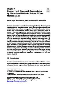
Fig. 2. Many-to-one ranking. Left: Cil is the union of three sub-shapes C1l−1 , C2l−1 , C3l−1 . Middle: M l−1 is the mean shape of C1l−1 , C2l−1 , C3l−1 . Right: Mapping of the ranking function Cil and M l−1 . Since the distance of Cil to the hyperplane is greater than that of M l−1 in this case, Cil is chosen as a better representation of the three sub-shapes. Each point of the triangle formed around M l−1 represents one of the three sub-shapes, and anywhere inside the triangle is a linear combination of the three shapes, with M l−1 as the centroid. function from any point to the hyperplane is: < w, ~ ~x > +b d(~x) = = ||w|| ~ 2
PNs i
α ~ i yi < ~xi , ~x > +b , PNs ~ i yi ~xi ||2 || i α
(1)
where b is the line intercept. If d > 0, ~x is more similar to the positive class and if d < 0, ~x is more similar to the neg~ n → H, be a mapping from ative class. In general, let Φ : R n ~ R to the Hilbert space H and K a kernel function defined as: K(~xi , ~xj ) =< Φ(xi ), Φ(xj ) >, then we can rewrite the signed distance function as: PNs d(~x) =
i
α ~ i yi < Φ(~xi ), Φ(~x) > +b . PN ~ i yi Φ(~xi )||2 || i s α
(2)
2.2. Shape Ranking The measure d induces a ranking function that we use to compare two given shapes as follows. Given two different shapes CA and CB , CA is more similar to the positive class than CB if d(CA ) > d(CB ). This can be understood by observing that ∆ = CB − CA implies d(∆) > 0. Now we generalize the notion of a one-to-one ranking to a many-to-one ranking with topological constraints and we will use it to construct a shape similarity tree. S T Consider Cil = Cjl−1 where Cjl−1 = ∅. Then we can express every shape Cjl−1 in terms of Cil as: d(Cjl−1 ) = d(Cil ) + d(∆jl−1 ).
(3)
We can rewrite this as: P P d(∆jl−1 ) d(Cjl−1 ) l − = µ(Cjl−1 ) − µ(∆l−1 d(Ci ) = j ), n n (4)
1297
B2