Classifying Graphs Using Theoretical Metrics: A Study of Feasibility

Classifying Graphs Using Theoretical Metrics: A Study of Feasibility Linhong Zhu1 , Wee Keong Ng2 , and Shuguo Han1 1 2

Institute for Infocomm Research, Singapore {LZHU,SHAN}@i2r.a-star.edu.sg Nanyang Technological University, Singapore {AWKNG}@ntu.edu.sg

Abstract. Graph classification has become an increasingly important research topic in recent years due to its wide applications. However, one interesting problem about how to classify graphs based on the implicit properties of graphs has not been studied yet. To address it, this paper first conducts an extensive study on existing graph theoretical metrics and also propose various novel metrics to discover implicit graph properties. We then apply feature selection techniques to discover a subset of discriminative metrics by considering domain knowledge. Two classifiers are proposed to classify the graphs based on the subset of features. The feasibility of graph classification based on the proposed graph metrics and techniques has been experimentally studied.

1

Introduction

The graph representations with a collection of nodes and edges support all aspects of the relational data analysis process. For instance, graphs can be used to represent chemical compound structures, program dependencies, protein-protein interactions, relationships in online social media and so on. In despite of the flourish of graph data, there is lack of efficient approaches for various classical graph theoretical problems. Among those, how to build an efficient automated graph classification models and identify discriminative graph features that separate different graph classes has valuable applications. For example, biologists are interested in studying whether a set of protein (a subgraph in protein-protein interaction network) is functional or not [11]. One conventional solution to classify graphs is first to compute the graph similarity using various measures such as graph-edit distance [3], maximum common subgraph [9] and canonical sequence similarity [2], and then decide whether they belong to the same cluster or not based on a pre-defined similarity threshold. Another solution is that one finds subgraph patterns as features [11,15,16,23] and then represents each graph as a feature vector. In this way, the graph classification problem is converted into the classification of traditional high dimensional data points. We refer the above two approaches as the isomorphism-based approach. They generally assume a hypothesis to verify the similarity of two graphs: If two J. Xu et al. (Eds.): DASFAA Workshops 2011, LNCS 6637, pp. 53–64, 2011. c Springer-Verlag Berlin Heidelberg 2011 

54

L. Zhu, W.K. Ng, and S. Han

graphs are similar in size/shape or they share a set of subgraph patterns, then they belong to the same cluster. As a result, graphs with the same cluster only differ from each other by a small number of nodes or edges. This hypothesis guarantees high accuracy for classification tasks for some particular domains, such as in the chemical data where size/shape differences of chemical component are small. However, this hypothesis is too restrictive to obtain outputs that are not similar in structure but highly related to each other, which can advance some domain analysis to gain significant benefits. As an example, in social network analysis, one interesting task is to predict a user’s gender by analyzing his/her connections to others. To address it, one first extracts a subgraph for each user induced by the user and his/her friends. Then the gender prediction problem is converted to graph classification problem. In this application, graphs for the same gender extremely vary in both size and the structure. However, they do share some implicit graph properties. For example, neighborhood graph of a female better fits the small-world phenomenon (popularly known as six degrees of separation [14]) than that of a man. In lieu of the above issue, this paper studies graph classification problem according to a more general hypothesis, i.e., if two graphs are similar in a set of diverse properties, then they belong to the same class. We call it “propertybased graph classification”. More specifically, we define the preliminary concept of property-based graph classification as follows. Problem 1. (Property-based Graph Classification) Given a graph G= (V , E) where V is a (finite) set of vertices and E is a (finite) set of edges, we assume that its properties could be measured by a set of graph theoretical-based metrics (More details about graph metrics will be given in Section 2.1). Then the property-based graph classification problem is to induce a mapping f (x): χ → {-1, 0, 1, . . ., γ}, from giving training samples T ={< xi , yi >}L i=1 , where xi ∈ χ represents properties of a graph G and yi ∈ {-1, 0, 1, . . ., γ} is a class label associated with training data, and L is the size of training samples. If yi ∈ {−1, 1}, we denote it as a binary property-based graph classification problem. The objectives of our work consist of two parts: (1) Investigating a set of graph theoretical metrics to facilitate graph classification; (2) Proposing an efficient and effective classification method for the property-based graph classification problem. The challenge lies not only in enumerating graph metrics, but also in selecting suitable metrics on the basis of domain knowledge. We address the challenges as follows: – We give an extensive survey about the most important and diverse graph metrics that have been proposed and used in a wide range of studies in multiple disciplines. We also propose five novel metrics, non-tree density, cut vertex density, connectivity, vertex compression ratio and edge compression ratio to further discover implicit properties. – Based on domain knowledge, we present an objective of feature selection combining with a greedy algorithm to perform discriminative feature subset selection.

Classifying Graphs Using Theoretical Metrics: A Study of Feasibility

55

– We explore an application of graph classification using graph metrics. We design two classifiers based on k-nearest neighbor classifier and reverse knearest neighbors classifier to verify the feasibility of graph classification using graph theoretical metrics. The organization of this paper is as follows: In Section 2, we enumerate a number of graph theoretical metrics and use them to transform graphs into feature vectors. We discuss how to build up graph classifiers in Section 3. In Section 4, we perform experiments to verify the feasibility of our approach. Finally, We review related work in Section 5 and conclude this work in Section 6.

2 2.1

Representing Graphs with Theoretical Metrics Graph-Theoretical Metrics

In the following definitions of metrics for graph properties, the definitions apply both to undirected and directed graph unless otherwise specified. In addition, we also provide the related references if they are not first proposed by this work. For easy representation, we use G to denote a single graph and G to denote a set of graphs. We simply use |V | to represent number of nodes and |E| to represent number of edges. Given two nodes u, v ∈ V , σ(u, v) denotes the distance (the length of shortest paths) from u to v. We use N (v, G) to denote a set of neighbors of v in graph G. Definition 1. (Global Clustering Coefficient [13]) The global clustering coeffi3Δ cient is defined as: GCC(G)= |(u,v,w):u,v,w∈V,u,v,wis connected| , where Δ is number of triangles. Global clustering coefficient is based on triplets of nodes. A triplet is three nodes that are connected by edges. A triangle consists of three closed triplets, one centrad on each of the nodes. The global clustering coefficient is 3 × triangles over the total number of triplets. Definition 2. (Characteristic Path Length [5]) Characteristic path length is de σ(u,v)

fined as CPL(G) = |V u,v |∗(|V |−1) . While characteristic path length is a measure of the average distance between any two nodes in the graph, global efficiency is a measure of the rate at which nodes can be reached from each other in the graph. It is approximately inversely related to characteristic path length. Definition 3. (Global Efficiency [20]) Global efficiency of a graph is defined as  GE(G)=

1 u,v σ(u,v)

|V |∗(|V |−1) .

Definition 4. (Degree Distribution [8]) The degree distribution of a graph is a function P : [0, . . ., kmax ] → [0, 1], where P (k) is the fraction of the vertices in G that have degree k for 0< k < kmax , and kmax is the largest degree in G.

56

L. Zhu, W.K. Ng, and S. Han

Definition 5. (Coreness [17]) The k-core of G is the largest subgraph Gk of G such that every vertex in Gk has at least k neighbors in Gk , i.e., ∀v ∈ V (Gk ), |N (v, Gk )| ≥ k. Definition 6. (Density) Given a graph G, we define its graph density as: ⎧ ⎨ |E|/|V |(|V | − 1) if G is directed, dg = ⎩ 2|E|/|V |(|V | − 1) if G is undirected. In addition, we propose two more density evaluation metrics, non-tree density and cut vertex density. Non-tree density dnt , is defined as |T |/|E|, where T is the set of non-tree edges, i.e., remaining edges after removing a spanning tree of a graph. Cut vertex density dc = |Vc |/|V | (where Vc is the set of cut vertices; i.e., articulation points) is the proportion of cut vertices. In the following metrics are restricted to directed graphs only. Definition 7. (Girth [7]) The girth of a graph is the length of the shortest cycle (of length >3) in the graph. Definition 8. (Circumference [7]) The circumference of a graph is the length of the longest cycle (of length >3) in the graph. Definition 9. (Connectivity) Connectivity |C| is the number of strongly connected component(s). Definition 10. (Vertex Compression Ratio) Vertex compression ratio rv =|V ∗ |/|V | (where |V ∗ | is number of vertices in condensed graph1 ) is the proportion of condensed graph vertices. Definition 11. (Edge Compression Ratio) Similar to Def. 10, edge compression ratio re =|E ∗ |/|E| (where |E ∗ | is number of edges in the condensed graph) is the proportion of condensed graph edges. Definition 12. (Acyclicity) de = |Ec |/|E| (Ec is the set of distinct edges that appear in a cycle) is a measure of the number of edges participating in one or more cycles. If there is no cycle, then |Ec | = 0. 2.2

Feature Selection and Graph Transformation

A graph can be viewed as a collection of features on the basis of above metrics. We may simply normalize the values of each features into the range [0, 1] and transform each graph into a feature vector. In the above setting, we just assume that each metric is equally important. In reality, however, it can not be true especially when considering applications in a specific domain. For example, in 1

We say G∗ =(V ∗ , E ∗ ) is a condensed graph of G if each vertex vi∗ ∈ V ∗ corresponds to a strongly connected component Ci in G, and each edge (vi , vj ) ∈ E ∗ if and only if there is at least one edge u, v ∈ E such that u ∈ Ci and v ∈ Cj .

Classifying Graphs Using Theoretical Metrics: A Study of Feasibility

57

social network analysis, a small-world network is mainly characterized by two metrics, namely, a shorter characteristic path length and a a higher clustering coefficient when compared to random graphs. Then a problem comes: given those aforementioned metrics, how can one select a subset of them to reduce the computation cost and achieve good classification performance? We refer it as a discriminative feature selection problem. In the following, we adopt similar technology from GSSC [12], to formulate the feature selection as an optimization problem. Next we discuss possible selection criteria and propose a greedy algorithm to solve the optimization problem. For simplicity, both term “feature” and “metric” are used to mention any of the aforementioned metrics. In addition, we use f to denote a single feature and F to denote a feature set. The numeric value of any feature over a graph G is denoted as f (G), and the combination of values of a set of features F over a −−−→ graph G is denoted as a vector F (G). Mathematically, discriminative feature selection problem could be formulated as: (1) Fd = arg max {R(T )} T ⊆F

where R(F ) is a measurement of discriminative over a set of features F . We investigate two principles that optimal features should have: representativeness and separability. This guides us to design a suitable discriminative measurement R. Separability means that graphs should be able to be separated from each other based on values of features; while representativeness is important to avoid selecting two highly correlated features. Both separability and representability are desirable in feature selection. Hence, we define R as a multi-criteria measurement: R(F ) = ω1 ρ(F ) − ω2

1 |F |



corr(fi , fj )

(2)

fi ,fj ∈F

where ρ(F ) denotes separability ratio of features set F , ω1 and ω2 are smoothing weights, and corr(fi , fj ) denotes correlation of two features fi and fj . Unfortunately, both separability ratio and feature correlation can be highly domain-dependant. As an example, we provide one possible design for measurements ρ(F ) and corr(fi , fj ) based on information of labeled background graphs. More specifically, let clustering C = {C1 , . . . , Cγ } denote the information of labeled background graphs, i.e., a cluster Ci ={G1 ,. . ., Gn } is a set of graphs that share the same class label yi ∈ {-1, 0, 1, . . . γ}. Then given clustering C, the separability ratio of a set of features F , is defined as ⎧ ⎫  −−−−→ ⎬ ⎨ || F (G )|| i ρ(F | C) = max log  Gi ∈C −−−−→ (3) C∈C ⎩ ||F (G )|| ⎭ Gj ∈C

j

It is clear that the larger the value of ρ(F | C), the better “worst-case” class separable capability feature set F is.

58

L. Zhu, W.K. Ng, and S. Han

Algorithm 1. Discriminative Feature Selection. Input: a clustering C of labeled graphs, a feature set F Output: a subset of features Fd 1: T = ∅, flag=true; 2: while flag 3: fk = arg maxf ∈(F \T ) {R(T ∪ {f } | C) − R(T | C)}; 4: if R(T ∪ {fk } | C) − R(T | C) > 0 5: T =T ∪ {fk }; 6: else 7: flag=false; 8: return T ;

Similarly, correlation of two features fi and fj given clustering C, is defined as corr(fi , fj | C) =

|X − E(X)||Y − E(Y )| σX σY

(4)

where the values of feature fi and fj over graphs in C are denoted as X and Y respectively. With respect to Equ. 1, we propose a greedy algorithm to solve it, as shown in Algorithm 1, we start with an empty set T = ∅, and in step k, iteratively add a feature fk such that it maximizes the margin gain fk = arg max {R(T ∪ {f } | C) − R(T | C)} f ∈(F \T )

(5)

Now given a graph G in a specific domain, we represent it as a feature vector using discriminative features. We also use the Euclidean distance to measure the −−−−→ −−−−→ dissimilarity of two graphs: dist(Gi , Gj ) = F (Gi ) − F (Gj )2 .

3

Graph Classification

In the previous section, we have discussed the features used to describe and represent graphs. In this section, with graph representation using theoretical metrics, we explore its potential in the domain of graph classification. Once graphs are converted into feature vector space, one can use traditional classifier to classify graphs. As a start, we build two classifiers which are similar to distance weighted knn classifier. Before we present the details of two classifiers, first let us introduce the notation of “knn” and “rknn”. For query graph G and the set of background graphs G, the set of k-nearest neighbors of G is the smallest set knn(G) such that knn(G)⊆ G, |knn(G)| ≥ k, and ∀Gi ⊆ knn(G), ∀Gj ⊆ (G\knn(G)): dist(G, Gi ) and a vector F  representing query graph → − Output: a class label y  representing classification of F  1: if knn classifier → − 2: Tnn =knn( F  , T ); → − 3: else Tnn =rknn( F  , T ); 4: initializing an array “vote” with length equal to number of classes γ; 5: for each tuple t ∈ Tnn 1 6: vote[t[1]]+= → − dist( F ,t[2])+

/∗ we use t[1] to denote the first entry of tuple t (i.e., the class label) and t[2] to denote the second entry of tuple t (i.e., a feature vector) ∗/ 7: return y  =arg maxi= 1 to γ vote[i]

Example 1. Let us consider an example shown in Figure 1. Figure 1(a) shows 4 graphs G1 , G2 , . . ., G4 , where each graph is assigned with a circle covering its two nearest neighbors. For example, 2nn(G1 )={G2 , G3 } and both G2 and G3 are enclosed in a circle with center G1 . Note that Gi ∈knn(Gj ) does not necessarily imply Gi ∈rknn(Gj ): G1 ∈2nn(G4 )={G1 , G3 }, but G1 ∈R2nn(G4 )={G3 }. In addition, for any given query G with k >= 1, knn(G) = ∅; while the set of reverse k-nearest neighbors rknn(G) might be empty. As shown in Figure 1(b),  2nn(G9 )={G1 , G7 }, but r2nn(G9 )=∅. From an abstract point of view, given a query graph, in the knn classifier, the algorithm finds the k most similar graphs in the training graph set. Then the weighted-based majority vote by the k most similar graphs, decides the classification. A rknn classifier is built in a similar way except that the weightedbased majority vote is done by the reverse k nearest neighbors. The details are shown in Algorithm 2. The feature vector representation of the → − query graph F  and sets of training feature vectors from each class y are fed to → − the classifier. Next, for F  , we perform either knn or rknn search to find a set of closest feature vectors and their class labels in the training set, denoted as Tnn (lines 1–3). After that, a distance weighted score is calculated for classification (lines 4–7). In line 6, we use a very small number  as a smoothing factor to avoid → − unbalance when the distance dist( F  , t[2]) is equal to 0. Note that for rknn

60

L. Zhu, W.K. Ng, and S. Han Table 1. Statistics of graph data Class # of graphs # of real graphs average |V | average |E| dual 139 22 11973 48481 interval 84 10 19996 106001 hopi 77 8 4886 16575

average dg 0.138874 0.009191 0.155612

classifier, Tnn may be empty (line 3). In this sense, the classification performance is the same with a random guess.

4

Experimental Evaluations

4.1

Tasks and Data Sets

We choose an interesting task from the query optimization area to evaluate our theoretical metric-based method for graph classification. The task is “graph reachability index selection”, which aims to decide a best index from a set of candidate reachability index. With the best index, graph reachability query performance could be significantly improved. The problem of “graph reachability index selection” can be formulated as a graph classification problem, where each class label is a type of graph reachability indexing. Specifically, one classifies two directed graphs into a same cluster if they share the same best reachability index. In our experiments, we choose interval approach [1], hopi [4] and dual labeling [22] as the set of candidate reachability indexing. We used both of real data and synthetic data in our experiments. All of the graphs are directed. For the real data, we used a set of real graphs obtained from a Web graph repository2 and papers [21,22]. In addition, we generated a set of synthetic graphs with two different graph generators. The first generator3 controls the graph properties with four input parameters: the maximum fanout of a spanning tree, the depth of a spanning tree, the percent of non-tree edges and number of cycles. The second generator4 generates a scale-free powerlaw graph, whose degree distribution follows a power-law function. The total number of graphs used is 300. For each graph, we manually labeled it with the best reachability index as follows: we pre-built each index on the graph and compared the total reachability query time of one million random queries. The best index is the one such that the total query cost is minimal. The statistics of graphs we used are summarized in Table 1. To measure the performance of our framework, we used the prediction accuracy A and micro precision P to measure the performance of our framework. The prediction accuracy A, is defined as A=Ti /n, where Ti is number of samples with right classification, and n is number of samples in total. The micro precision 2 3 4

http://vlado.fmf.uni-lj.si/pub/networks/data/ http://www.cais.ntu.edu.sg/~ linhong/gen.rar http://www.cais.ntu.edu.sg/~ linhong/GTgraph.zip

Classifying Graphs Using Theoretical Metrics: A Study of Feasibility

61

Table 2. Running time and memory usage of feature selection Running time (seconds) Memory usage (MB) Metric computation Feature selection Metric computation feature selection 50.373 24.035 89.83 3.8

P is defined as

γ  i=1

T Pi /

γ 

(T Pi + F Pi ), where γ is number of class labels, T P

i=1

is the true positive, and F P is the false positive. 4.2

Results

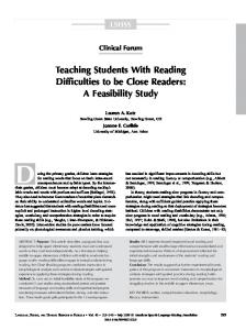
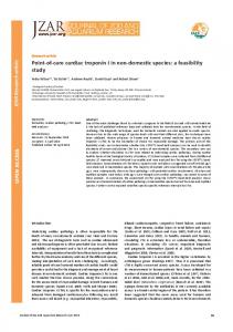
Discriminative features. For the specific task of “reachability index selection”, the set of discriminative features that returned by Algorithm 1 are: 1) Nontree density; 2) Degree distribution; 3) Global efficiency; 4) Diameter; 5) Vertex compression ratio; 6) Coreness; 7) Global clustering coefficient; and 8) Graph density. Next we report the total running time and memory usage of two stages in discriminative feature selection: I) computing graph metrics (See Sec 2.1), and II) discriminative feature selection (See Algorithm 1). The results are shown in Table 2. It is observed that the memory usage is dominated by Stage I, i.e, the storage consumption to keep the whole graph in the memory. Interestingly, running time is also mainly taken up by the first stage. The reason is that we need to compute 14 metrics for each graph in the first stage and each metric computation needs to be done at least in linear time to the graph size. Classification Performance. We randomly chose NT number of test graphs both from real graphs and synthetic graphs, where NT varies from 20 to 100. In addition, in average, the first i graphs are more similar to the training graphs than the fist j graphs (i < j). The total running time and memory usage of knn and rknn classifiers, are presented in Figure 2. The result shows that though knn approach is faster than rknn approach, the margin is quite small. Figure 2(b) reports the memory usage (excluding the memory consumption to keep graphs) comparison of two approaches. It implies that each approach is comparable to another in memory consumption. Figure 3 gives the prediction accuracy and micro-precision when number of test graphs is varied. Despite knn classifier gets higher accuracy on a small number of testing graphs that are highly similar to training graphs, in average, rknn classifier obtains substantial improvement than knn approach in classification accuracy. The results indicate that knn classifier are more vulnerable to the quality of training graphs than rknn classifier: when training graphs are noticeably similar to testing graphs, knn classifier could get classification of good quality; when training graphs are relatively dissimilar to testing graphs, the performance of knn drops off sharply. On another hand, we also observe that the performance of knn is more stable than that of rknn. The reason is that there is no guarantee for the existence of rknn search results. Hence, the weighted major vote on an empty set would trigger a random guess (see Algorithm 2).

62

L. Zhu, W.K. Ng, and S. Han Total running time (seconds)

Memory consumption (KB) 7000

KNN RKNN

14 12

KNN RKNN

6000 5000

10 8

4000

6

3000

4

2000

2

1000

0

0 20

30

40 50 60 70 80 Number of testing graphs

90

100

20

(a) Running time comparison.

30

40 50 60 70 80 Number of testing graphs

90

100

(b) Memory usage comparison.

Fig. 2. Performance comparison Classification Accuracy 0.9 KNN 0.85 RKNN 0.8 0.75 0.7 0.65 0.6 0.55 0.5 20 30

Micro-precision 0.8 0.7 0.6 0.5 0.4 0.3 KNN RKNN

0.2 0.1 40 50 60 70 80 Number of testing graphs

90

100

20

30

40 50 60 70 80 Number of testing graphs

90

100

Fig. 3. Prediction accuracy and micro-precision comparison

We attain similar results of micro precision of these two classifiers. Based on Figure 3, we can draw a conclusion that graph classification using theoretical metric is feasible since the accuracy of both two classifiers is much higher than random guess (33.3%).

5

Related Work

Related works about graph classification are mainly in the field of subgraph pattern selection and graph pseudo-isomorphism testing. If we could have a set of subgraph patterns, graphs can be represented as feature vectors of patterns and graph classification problem is converted into traditional data classification problem. In subgraph pattern selection, the major difficulty of this approach is to find informative subgraph patterns efficiently. The pioneer work [6] starts to find frequent subgraph patterns to represent graphs. One drawback of frequent subgraph pattern representation is that one can find a tremendously large quantity of frequent patterns in a large graph, which leads to relatively poor scalability. Later, Leap [23], gPLS [16], CORK [19], graphSig [15] and GAIA [11] propose to search directly for discriminative subgraph patterns that can better assist graph classification. A recent work COM [10] makes use of co-occurrences of subgraph patterns to improve graph classification performance.

Classifying Graphs Using Theoretical Metrics: A Study of Feasibility

63

Another direction of graph classification relies on pseudo-isomorphism testing (graph similarity measure). Various degree of matching metrics such as graphedit distance [3], maximum common subgraph [9], canonical sequence similarity [2] and so on have been proposed and used to assist graph classification. These approaches are theoretically sound and can guarantee optimal or near-optimal solutions in some sense. However, computing graph-edit distance or maximum common subgraph itself is really time-consuming due to their intractability. Recently, Zeng et al. [24] propose a solution to compute the lower bound and upper bound of graph-edit distance in polynomial time to facilitate graph similarity search as well as graph classification. Unfortunately, the above works are mainly in the area of chemical and biological data. In addition, all of them are proposed for the isomorphism-based graph classification problem. Although the problem of property-based graph classification is important in practice for applications in social network analysis, database design and query optimization, we are not aware of any focused study of this problem.

6

Conclusions

In this paper, we formalized the problem of property-based graph classification. Upon this formalization, we studied the feasibility of graph classification using a number of graph theatrical metrics. We also proposed a greedy algorithm to select a set of discriminative metrics. Experimental results showed that our framework works good in terms of both accuracy and micro precision, which verified the possibility of graph classification using graph metrics.

References 1. Agrawal, R., Borgida, A., Jagadish, H.V.: Efficient management of transitive relationships in large data and knowledge bases. In: Proceedings of the 1989 ACM International Conference on Management of Data, pp. 253–262. ACM, New York (1989) 2. Babai, L., Luks, E.M.: Canonical labeling of graphs. In: Proceedings of the 15th Annual ACM Symposium on Theory of Computing, pp. 171–183. ACM, New York (1983) 3. Bunke, H.: On a relation between graph edit distance and maximum common subgraph. Pattern Recognition Letters 18(9), 689–694 (1997) 4. Cheng, J., Yu, J.X., Lin, X., Wang, H., Yu, P.S.: Fast computation of reachability labeling for large graphs. In: Ioannidis, Y., Scholl, M.H., Schmidt, J.W., Matthes, F., Hatzopoulos, M., B¨ ohm, K., Kemper, A., Grust, T., B¨ ohm, C. (eds.) EDBT 2006. LNCS, vol. 3896, pp. 961–979. Springer, Heidelberg (2006) 5. Coffman, T.R., Marcus, S.E.: Dynamic classification of groups through social network analysis and hmms. In: IEEE Aerospace Conference, pp. 3197–3205 (2004) 6. Deshpande, M., Kuramochi, M., Wale, N., Karypis, G.: Frequent substructurebased approaches for classifying chemical compounds. IEEE Transaction on Knowledge and Data Engineering 17(8), 1036–1050 (2005)

64

L. Zhu, W.K. Ng, and S. Han

7. Diestel, R.: Graph Theory, 3rd edn., vol. 173. Springer, Heidelberg (2005) 8. Faloutsos, M., Yang, Q., Siganos, G., Lonardi, S.: Evolution versus intelligent design: comparing the topology of protein-protein interaction networks to the internet. In: Proceedings of the LSS Computational Systems Bioinformatics Conference, Stanford, CA, pp. 299–310 (2006) 9. Montes-y-G´ omez, M., L´ opez-L´ opez, A., Gelbukh, A.: Information retrieval with conceptual graph matching. In: Ibrahim, M., K¨ ung, J., Revell, N. (eds.) DEXA 2000. LNCS, vol. 1873, pp. 312–321. Springer, Heidelberg (2000) 10. Jin, N., Young, C., Wang, W.: Graph classification based on pattern co-occurrence. In: Proceeding of the 18th ACM Conference on Information and Knowledge Management, pp. 573–582. ACM, New York (2009) 11. Jin, N., Young, C., Wang, W.: Gaia: graph classification using evolutionary computation. In: Proceedings of the 2010 International Conference on Management of Data, pp. 879–890. ACM, New York (2010) 12. Kong, X., Yu, P.S.: Semi-supervised feature selection for graph classification. In: Proceedings of the 16th ACM International Conference on Knowledge Discovery and Data Mining, pp. 793–802. ACM, New York (2010) 13. Luce, R., Perry, A.: A method of matrix analysis of group structure. Psychometrika 14(2), 95–116 (1949) 14. Milgram, S.: The Small World Problem. Psychology Today 2, 60–67 (1967) 15. Ranu, S., Singh, A.K.: Graphsig: A scalable approach to mining significant subgraphs in large graph databases. In: Proceedings of the 2009 IEEE International Conference on Data Engineering, pp. 844–855. IEEE Computer Society, Washington, DC, USA (2009) 16. Saigo, H., Kr¨ amer, N., Tsuda, K.: Partial least squares regression for graph mining. In: Proceeding of the 14th ACM International Conference on Knowledge Discovery and Data Mining, pp. 578–586. ACM, New York (2008) 17. Seidman, S.B.: Network structure and minimum degre. Social Networks 5, 269–287 (1983) 18. Tao, Y., Papadias, D., Lian, X.: Reverse knn search in arbitrary dimensionality. In: Proceedings of the 30th International Conference on Very Large Data Bases, pp. 744–755. Very Large Data Bases Endowment (2004) 19. Thoma, M., Cheng, H., Gretton, A., Han, J., Peter Kriegel, H., Smola, A., Song, L., Yu, P.S., Yan, X., Borgwardt, K.: Near-optimal supervised feature selection among frequent subgraphs. In: SIAM Int’l Conf. on Data Mining (2009) 20. Thomason, B.E., Coffman, T.R., Marcus, S.E.: Sensitivity of social network analysis metrics to observation noise. In: IEEE Aerospace Conference, pp. 3206– 3216 (2004) 21. University of Michigan: The origin of power-laws in internet topologies revisited. Web page, http://topology.eecs.umich.edu/data.html 22. Wang, H., He, H., Yang, J., Yu, P.S., Yu, J.X.: Dual labeling: Answering graph reachability queries in constant time. In: Proceedings of the 22nd International Conference on Data Engineering, p. 75. IEEE Computer Society, Washington, DC, USA (2006) 23. Yan, X., Cheng, H., Han, J., Yu, P.S.: Mining significant graph patterns by leap search. In: Proceedings of the 2008 ACM International Conference on Management of Data, pp. 433–444. ACM, New York (2008) 24. Zeng, Z., Tung, A.K.H., Wang, J., Feng, J., Zhou, L.: Comparing stars: on approximating graph edit distance. Proc. VLDB Endow. 2, 25–36 (2009)