Cognitive Computation: a Bayesian Machine Case Study Marvin FAIX, Emmanuel M AZER LIG - Université de Grenoble, France Email:
[email protected] [email protected]
Raphaël L AURENT, Mohamad OTHMAN A BDALLAH, Ronan L E H Y ProbaYes, Grenoble, France Email:
[email protected]
Abstract—The work presented in this paper is part of the BAMBI project, which aims at better understanding natural cognition by designing non Von Neumann machines with biologicaly plausible hardware. Probabilistic programming allows artificial systems to better operate with uncertainty, and stochastic arithmetic provides a way to carry out approximate computations with few resources. As such, both are plausible models for natural cognition. Our work on the automatic design of probabilistic machines computing soft inferences with an arithmetic based on stochastic bitstreams allowed us to develop the following compilation toolchain: given a high level description of some general problem (typically to infer some knowledge from a model given some observations), formalized as a Bayesian Program, our toolchain automatically builds a low level description of an electronic circuit computing the corresponding probabilistic inference. This circuit can then be implemented and tested on reconfigurable logic. We designed as a validating example a circuit description of a Bayesian filter solving the problem of Pseudo Noise sequence acquisition in telecommunications.
I.
Jorge L OBO Institute of Systems and Robotics University of Coimbra, Portugal Email:
[email protected]
I NTRODUCTION
The present study is a subproject of BAMBI (Bottomup Approaches to Machines dedicated to Bayesian Inference (www.bambi-fet.eu): a European collaborative research project relying on the theory of Bayesian inference as a tool to understand natural cognition and aiming at designing bioinspired computing devices. The main hypothesis underpinning the project is that, since living beings are using energy efficient information processing systems able to cope with uncertainty, Bayesian models may account for some of their abilities at the macroscopic level. For example, Bayesian models for language learning, behavior prediction or decision making are numerous in human studies [1]. Indeed, effective perception and decision making need to take into account the intrinsic incompleteness of any world representation. This can be done optimally with Bayesian inference [2]. Complementary to these rather macroscopic approaches, the bottom-up approach adopted within the framework of BAMBI is to study how probabilistic inference can be made at the biochemical scale and how biochemical cascades of cell signaling can perform the necessary probabilistic computations [3]. The BAMBI project includes testing these hypotheses on Chlamydomonas reinhardtii, a wellstudied mobile unicellular microalga. Should our hypothesis hold, then we further conjecture that probabilities are coded with binary telegraphic signals: this is supported by the fact that the extremely fast conformation transitions of alosteric molecules, which govern the exchange of information inside
the cell, can be modeled by Poisson processes. Extending this bottom-up approach to artifacts, the goal of the project is to design electronic machines based on similar principles. Here are the objectives that we set for such a machine: it needs to take into account the uncertainty of its inputs, to be fault tolerant, and to meet low power needs. The purpose of this paper is to present our initial solution: we automatically generate electronic circuits to carry out Bayesian inference, which are based on the temporal coding of probability values as bitstreams, run without floating point unit arithmetic, and are very lightened in terms of electronic components. As an illustrating example, we selected the design of a Bayesian filter which devises categories out of a noisy temporal series. The paper is organized as follows. After presenting similar approaches in the literature, we show how Bayesian Programs are used to specify inferences and how we compile them into specifications for the appropriate circuit. We present a set of logic operators to perform the arithmetic operations with stochastic logic. Then we describe our toolchain that starts with a Bayesian Program and generates a hardware description program in VHDL (VHSIC Hardware Description Language, where VHSIC stands for Very High Speed Integrated Circuit) describing the corresponding Bayesian inference machine which has been implemented and tested on reconfigurable logic hardware: FPGA (Field-Programmable Gate Array). We illustrate the working of the obtained machine on a simple inference example, which allows to highlight a fundamental problem with the temporal coding of probabilities: the time dilution of probabilities during the inference process. A solution to this problem is presented and illustrated through a more complex example: the design of an electronic implementation of a Bayesian Filter aimed at solving the problem of Pseudo Noise sequence acquisition in telecommunications. II.
R ELATED W ORKS
Probabilistic inference and learning are now used in many applications ranging from robotics [4][5][6] to cognitive modeling [1] and machine learning [7]. Designing a general purpose and high level language to program these applications has been an objective for many research teams. One particular aspect of this research is the design of probabilistic languages where inference and learning are built within the interpretor of the language itself: ProBT[8][9], Figaro[10], Blog[11] are a
few examples of such programming languages. One emerging goal is to build dedicated hardware to interpret these languages and perform fast probabilistic inferences using energy efficient hardware. For instance, the works of Vigoda [12], Mansinghka[13] and Jonas [14] describe hardware architectures dedicated to probabilistic inference. Vigoda [12] uses continuous time analog circuits. Analog values represent probability values and his architecture derives from the message passing algorithm [15] to propagate uncertainty and compute the probabilistic inferences. Unlike Jonas [14] and Mansinghka[13], Vigoda’s system performs exact inferences by analog means. Mansinghka was both interested in the programming and in the design of probabilistic machines. He first designed the probabilistic programming language Church [16] and showed how to compile the specification written in Church into an electronic circuit. Mansinghka [13] followed by Jonas [14] performed approximate inference by using samplers to represent probability distributions and by using Metropolis like algorithms. Contrary to these approaches, we choose to use a stochastic arithmetic to perform the algebraic operations required by probabilistic inference. This is motivated by our bio inspired approach to use stochastic time coding sequences for representing probabilities. Early in 1956, Von Neumann [17] had already considered the design of a computer based on probabilistic arithmetic but it is in 1967 that Gaines [18] popularized the term stochastic computing. The simplicity of the involved logical arithmetic operations (additions and multiplications) is one of the main strength of this approach, but computation time and accuracy of the results held back the development of advanced probabilistic hardware. However, the use of probabilistic models of computation is nowadays experiencing a renewed interest from the scientific community. Indeed, a major advantage of inherently probabilistic circuits is that they are more robust, fault tolerant and that they can be used to compute any function (see for instance [19][20]). A simple argument supports this: with a standard representation of a probability value, if a bit-flip occurs on the most significant bit, then the result is very different from the original value. With a bitstream representation, each bit has the same weight. This means that a bit-flip is much less important for the result, and several bit-flips may compensate one another, which makes bitstream representations of probability values intrinsically more robust to noise. Besides, some designers are also using probabilities to lower the voltage and thus the power supply of such circuits. For example, the PCMOS [21] project uses a probabilistic extension of the boolean logic to limit the global error due to the probabilistic behaviour of individual logical components. Our work shares some common objectives with the IBM TrueNorth project [22] as both aim at designing non-von Neumann bio-inspired energy efficient information processing systems. TrueNorth proposes a neuromorphic architecture where the building blocks are neurons which are implemented in a rather classical way (they use fixed point arithmetic units to compute a neuron’s output from its inputs with various neural activation codes: binary, rate, population, and time-tospike). The approach of the BAMBI project differs from this
in at least two ways. First, we follow Jayne’s idea that the use of probabilities is a natural candidate to handle the uncertainty inherent to any subjective reasoning [2], which we do within a well defined formalism [9]. Indeed, probabilities are central to our work, and in this paper we describe the automatic design of hardware realizing probabilistic computations with a stochastic arithmetic based on a temporal coding of probabilities. Second, our bio-inspiration comes from the nanoscopic scale (as opposed to microscopic for neurons) where it has been shown by studying intracellular messaging how simple biochemical interactions underlie simple probabilistic inferences [3]. III. F ROM BAYESIAN P ROGRAMS TO H ARDWARE I MPLEMENTATIONS OF BAYESIAN M ACHINES A. Specifying a Bayesian Machine from a Bayesian Program A Bayesian machine can be rigorously defined within the Bayesian Programming formalism [9]. Such a machine computes soft inferences by taking probability distributions as inputs, which are called soft evidences, from which it computes the output probability distribution. We have designed a compiler allowing to compute an electronic circuit implementation of any such Bayesian machine from a specification written in the language ProBT [8][9]. We give here an example of such a definition, which will be used later in the paper. We consider a joint probability distribution on a set of discrete and finite variables: P (M ∧ D ∧ L). Where M, D and L are themselves conjunctions of variables, for example D = D1 ∧ . . . ∧ Dk . We define the soft evidences on the variables Dk as the probability distribution P˜ (Dk ). These soft evidences will be the inputs of the Bayesian machine. Given the soft evidences P˜ (Dk ) and the joint distribution P (M ∧D ∧L), we ask the machine to compute the probability distribution over M , which is done by Bayesian inference: X X 1 X 0 P (M ) =
Z
P˜ (D1 ) . . .
D1
P˜ (Dk )
Dk
L
where Z is a normalization constant: X X X X P˜ (D1 ) . . .
Z=
M
D1
P˜ (Dk )
Dk
L
P (M ∧ D ∧ L) , (1)
P (M ∧ D ∧ L)
!
. (2)
In other words, the machine computes a soft inference based on the joint probability distribution P (M ∧ D ∧ L). The Bayesian machine is defined by writting specifications of its joint probability distribution, inputs and output in the ProBT language [8]. Figure 1 shows the simple specification of our example using the Python bindings of ProBT1 . This program expresses explicit conditionnal independance hypotheses allowing to simplify the computation of the joint probability distribution (see figure 1, line 21): P (M ∧ D1 ∧ D2 ) = P (M )P (D1 |M )P (D2 |M ) . It also specifies the output M and the inputs D1 and D2 of the machine. No latent variables L are given in this example but they can be handled too (see the filter example in section IV). The last instruction of this program will produce an internal simplification of expression (1) which minimizes the 1 A free version of ProBT is available at http://www.probayes.com/ fr/Bayesian-Programming-Book/downloads/.
1
5
9
13
17
21
25
P˜ (D1 )
# import the ProBT bindings from pypl import * # define the variables dim3 = plIntegerType(0,2) D1 = plSymbol(’D1’,dim3) D2 = plSymbol(’D2’,dim3) M = plSymbol(’M’,dim3) # define the distribution on M PM = plProbTable(M,[0.8,0.1,0.1]) # define a conditional distribution on D1 PD1_k_M = plDistributionTable(D1,M) PD1_k_M.push(plProbTable(D1,[0.5,0.2,0.3]),0) PD1_k_M.push(plProbTable(D1,[0.5,0.3,0.2]),1) PD1_k_M.push(plProbTable(D1,[0.4,0.3,0.3]),2) # define a conditional distribution on D2 PD2_k_M = plDistributionTable(D2,M) PD2_k_M.push(plProbTable(D2,[0.2,0.6,0.2]),0) PD2_k_M.push(plProbTable(D2,[0.6,0.3,0.1]),1) PD2_k_M.push(plProbTable(D2,[0.3,0.6,0.1]),2) # define the joint distribution model = plJointDistribution(PM*PD1_k_M*PD2_k_M) # define the soft evidence variables model.set_soft_evidence_variables(D1^D2) # define the output question = model.ask(M)
11000101100
11000101100
P (M)
Z
D1
P˜ (D1 )P (D1 |M ))(
D2
P˜ (D1 )P (D1 |m2 ))(
D2
P˜ (D2 )P (D2 |m2 ))
11000101100
P ′ (M|P˜ (D1 )P˜ (D2 ))
P (D1 |M)
P (D2 |M)
Fig. 2. The probabilistic machine corresponding to the given program: its inputs are the soft evidences (arrows incoming from the left) and its output is the probability distribution over the variable of interest M . The probability values of the internal parameters of the terms of the joint distribution are set by a set of TRNGs (True Random Number Generators) and the symbolic expression used to compute the inference is produced by the SRA algorithm.
arithmetic. In this section we show how these probabilistic operators can be implemented so that their output bitstream encodes the appropriate probability values. 1) Stochastic Bitstreams and Stochastic Buses: Stochastic bitstreams may be used to code rational numbers in the interval [0, 1]. If we observe a bitstream of length N and count the number N1 of bits set to one, the bitstream will code for cj ∈ [0, 1] if NN1 → cj when N → ∞. A set of n stochastic bitstreams implicitly code for a probability distribution over a discrete probabilistic variable X by normalizing the values ci represented by each bitstream: . So, a probability distribution on a P (X = xi ) = Pnci c j=1
j
variable X can be coded with a set of n = card(X) stochastic bitstreams which form what we call a “probabilistic bus”. Basic arithmetic operations on stochastic bitstreams can be done using single logic gates [18] [24].
P (M ∧ D1 ∧ D2 ) = P (M )P (D1 |M )P (D2 |M ) , P (M )(
D1
Biased TRNGs
computational load by reducing the number of sums according to the structure of the joint distribution. The algorithm used to produce this simplification is the Successive Reductions Algorithm (SRA) [8], which is an algorithm similar to the sumproduct [15] algorithm. For example, in the program above, since the joint probability distribution is specified as
P (M ) =
P P P˜ (D1 )P (D1 |m0 ))( D2 P˜ (D2 )P (D2 |m0 )) P PD1 ˜ P (D1 )P (D1 |m1 ))( D2 P˜ (D2 )P (D2 |m1 )) D1 P P
P˜ (D2 )
Fig. 1. Specification of a Bayesian Program using the python bindings for ProBT. It is comprised of the variable definitions, the definition of the joint probability distribution over all considered variables as a product of simpler distributions (see line 21), the specification of values for the parameters of these distributions, and a question asked to the model (see line 25), which will be solved by Bayesian inference.
the SRA will transform equation (1) into: X X 1 0
1 P (m0 )( Z 1 P (m1 )( Z 1 P (m2 )( Z
P˜ (D2 )P (D2 |M )) . (3)
Figure 2 presents the high-level representation of the architecture for the Bayesian Machine. It comprises the main stochastic machine along with the True Random Generators (TRNG) [23] generating the stochastic bitstreams encoding the probability values of the constants considered in the problem. While TRNGs normally produce uniform bitstreams, they are biased so as to output the desired probability values. These constants represent the knowledge encoded in the model. B. Basic Stochastic Logic Arithmetic It is a general result of Bayesian inference that any probability distribution can be computed from the decomposition of the joint probability distribution (yielding results similar to the example shown in equation (3)) and that this computation only involves standard mathematical operators: multiplication, addition and division. The ease of implementation of such operators, with a representation of the probability values as bitstreams, is precisely a key strength of using a probabilistic
2) Stochastic Products: Computing a multiplication over two probability values is easy: it only requires to use an “AND” gate. Indeed, if two independent bitstreams coding for c1 and c2 are the inputs of an “AND” gate then the output bitstream encodes the value c1 c2 [19]. 3) Stochastic Addition with a Multiplexer: The average of two stochastic bitstreams can be computed simply as their multiplexing using a stochastic selector, if they are uncorrelated. If n independent bitstreams coding for c1 . . . cn are the inputs of a multiplexer Pn with a round counter selector, then the cj
j=1 : a scaled sum that corresponds to output codes for n the average of the inputs. Still, if we use the multiplexer to add two probability values we have to face the problem of the time dilution of probabilities. Indeed, if we note b1 and b2 the bitstream representations of p1 and p2 , multiplexing 2 b1 and b2 produces the output s = p1 +p 2 , and, for n input n . Dividing by n reduces the number signals, s = p1 +p2 +...+p n of ones in the resulting bitstream. This problem could become increasingly important if the inference needs nested sums. For example, if the inference cascades 4 sums with n1 = 5, n2 = 10, n3 = 8 and n4 = 10 then the result will be divided by 4000! So the resulting bitstream will have to be observed for a long time before getting a good approximation of the
probability value encoded in the result. To solve this problem (encountered while studying the simple application described in section III-C) we designed another adder using a simple OR gate combined with a counter. 4) Addition with an “OR” Gate and a Memory: As in our approach we compute probability distributions, the result of the summation never exceeds 1, by definition. Since a probability value is defined as the number of 1 in its bitstream representation over the bitstream length, adding two or several probabilities amounts to counting the number of 1 of each bitstream encoding the probability values. We design a component specified by the truth table shown figure 3. inputs 00 01 10 11
output 0 1 1 1
R=0 0 0 0 1
inputs 00 01 10 11
output 1 1 1 1
generated by the proposed toolchain. More precisely, figure 4 (bottom) shows the RTL (Register Transfer Level) description generated by the synthesis tool, where it is possible to identify the connections between the components, corresponding to the logical circuit in figure 4 (up).
R 6= 0 R−1 R R R+1
Fig. 3. The truth tables of a two input OR gate with memory (OR+). In both tables, the rightmost column contains the updated value of the counter R. For the left table, the previous state is R = 0 while for the right table, previously R > 0.
The classical OR gate’s output is 1 if one of the input is 1. A problem arises when two inputs are simultaneously set to 1. In this case a counter R is incremented. If all of the inputs are 0, the output is 0 excepted if the counter is different from 0, then we output a 1 and the counter is decremented. In other words, we reintroduce the forgotten bits as soon as it is possible. By adding a counter to a traditionnal OR gate, we obtain our stochastic adder, which we name OR+, for OR gate with memory. C. Initial Evaluation of a simple Architecture In this section we describe in more detail how equation (3) is evaluated in terms of logical components and circuit implementation. Each probability distribution of expression(3) is coded with a probabilistic bus. We distinguish the soft evidences, which are the inputs of the probabilistic machine, from the probability distributions defining the joint distribution over all variables. The inputs may change while the other distributions are set by the programmer as internal parameters when specifying the joint distribution. Biased TRNGs (True Random Number Generators) are used to produce the probabilistic buses associated to these distributions (see figure 2). For example, in expression (3), P (D1 |M = m) is represented by a stochastic bus with three stochastic signals c0 = k ∗ P (d01 |m), c1 = k ∗ P (d11 |m) and c2 = k ∗ P (d21 |m), and so, three biased TRNGs are used to produce the stochastic bitstreams representing c0 , c1 and c2 . The compilation itself is done by (i) using ProBT to compute the formula (see expression (3)) corresponding to the probabilistic question asked in the Bayesian Program (see figure 1), and (ii) by parsing the obtained formula to generate a circuit description performing the necessary sums and products using standard logic. Since, by nature of Bayesian inference, the resulting circuit architecture duplicates several times some subblocks, for the sake of readability we show on figure 4 the subpart P of the generated circuit which computes the sub˜ expression D1 P (D1 )P (D1 |M = m) of expression (3). This figure is a graphical representation of the VHDL code
P
Fig. 4. Stochastic circuit computing 13 P˜ (D1 )P (D1 |m) and the D1 corresponding RTL (Register Transfer Level) description.
Since the structure of expression (3) is independent of any particular value m of M , the circuit generated to compute each output m of M has exactly the same structure. As a consequence, the weights introduced by the multiplexers will cancel out during normalisation and P’(M) can be correctly computed from the outputs. D. First Validating Results with a Simple Machine The proposed toolchain is working and accepts any ProBT program with discrete variables as entry. The toolchain generates a VHDL file which is the description of the stochastic circuit and can be implemented on a FPGA (FieldProgrammable Gate Array; a FPGA is a piece of hardware the logic of which can be configured, which we use so as to implement our circuit). A Cyclone IV FPGA from Altera has been targeted as supporting device. A machine has been synthesized to demonstrate the applicability and scalability of the proposed toolchain. Besides, ProBT is also used to compute the exact result using standard arithmetic. This gives a ground truth allowing to evaluate the results given by the FPGA implementation of the synthesised VHDL program. Here we describe preliminary results which were obtained with software generated random bitstreams, which are less temporally correlated than what current off the shelf hardware TRNGs (True Random Number Generators) produce.
To simulate the circuit computations we need to specify two sets of probability values. First, the internal parameters of the model: the parameters of the terms of the joint distribution encoding the model knowledge relevant for the inference computed by the considered circuit. These parameters are hardcoded into the circuit once and for all. Second, the circuit inputs: probability distributions encoding soft evidences, i.e. probability distributions quantifying a relative confidence over observations. These inputs are variables which may change over time. All these parameters are set as is shown table I.
0.25 0.20
Error (RMSE)
We simulate the computations carried out by the electronic circuit resulting from the compilation of the Bayesian Program described by figure 1. As probability values are represented as bitstreams, the length of the streams, i.e. the number of bits used to encode a probability value, obviously has a direct impact on the precision of the encoded values and consequently on the precision of the computations realized by a given circuit. The goal of the following simulations is twofold: (i) to validate the fact that the circuits generated by our toolchain that compiles Bayesian Programs into hardware representations correctly outputs electronic circuits computing the appropriate results, and (ii) to quantify the impact of the bitstream length on the precision of the overall computations.
0.15 0.10 0.05 0.00
50
200
800
0 0 0 0 320 1280 5120 20480
Bitstream size Fig. 5.
Evolution of the RMSE as a function of the bitstream length.
bitstream size P(Best) RMSE
50 0.801 0.21
200 0.723 0.11
800 0.724 0.06
3200 0.715 0.02
12800 0.714 0.008
51200 0.710 0.0034
204800 0.711 0.0035
reference 0.711 0
TABLE II.
C ONVERGENCE OF THE CIRCUIT SIMULATION OUTPUTS TOWARDS THE THEORETICAL VALUE ( RIGHTMOST COLUMN ).
Internal parameters name value
P (d01 |m0 ) 0.2
P (d11 |m0 ) 0.3
P (d21 |m0 ) 0.5
P (d01 |m1 ) 0.3
P (d11 |m1 ) 0.2
Internal parameters name value
P (d21 |m1 ) 0.5
P (d01 |m2 ) 0.4
P (d11 |m2 ) 0.3
P (d21 |m2 ) 0.3
Inputs name value
TABLE I.
P˜ (d01 ) 0.8
P˜ (d11 ) 0.1
P˜ (d21 ) 0.1
P˜ (d02 ) 0.8
P˜ (d12 ) 0.1
P˜ (d22 ) 0.1
T HE MODEL INTERNAL PARAMETERS AND INPUTS USED IN OUR SIMULATIONS .
Having set these probability values, we simulate the behavior of the circuit, which computes P 0 (M ) = P (M | P˜ (D1 ) P˜ (D2 )), according to the formula shown equation (3). To compare with the theoretical values obtained thanks to ProBT, we use the standard Root Mean Square Error (RMSE) to measure the difference between the best guess probability as computed by our circuit and its theoretical value. Figure 5 shows how this error, computed on ten simulations with different random seeds, evolves when the length of the simulated bitstreams increases. Figure 5 shows that the error globally decreases when the bitstream size increases. This means that our simulated circuit successfully computes the appropriate values. Still, this progressive increase in precision of the computed result is rather slow , and it is necessary to consider streams of several thousands bits to have errors of less than 1%. Indeed, since bitstreams of size N drawn to encode a probability value . p are Bernouilli sequences, their variance is σ 2√ = p(1−p) N This means precision increases at the rate O(1/ N ), which is comparable to the data of figure 5. Table II shows in more detail the outputs of the simulation which allowed to plot figure 5.
It is interesting to note three things. First, our error measure is such that differences in opposed directions do not compensate. As a consequence the average value of the best guess probability seems to converge faster than the error. Second, for bitstreams of size 204800, the error is larger than for bitstreams of size 51200. This might be because we compute averages on 10 simulations only, which introduces some kind of noise around the theoretical values. For large bitstream sizes, the error is low and only this noise is observed. And third, for small bitstream sizes the error is rather big, but the corresponding bias is in favor of the most probable answer. This is because with small stream sizes lower probabilities are underestimated (for instance, to code a probability value of 0.1%, it is necessary to have a bitstream of size 1000 to observe in average one non zero bit). Having this favorable bias towards most likely outcomes with small bitstreams results in a system which is “too sure of itself”: it makes faster decisions, at the cost of low probability events underestimation. IV.
D ESIGNING A S TOCHASTIC BAYESIAN F ILTER
In our previous example, the definition of a probabilistic bus allowed us to compute the output distribution without computing the normalization constant Z (see equation (2)). In addition, we used a simple multiplexer to perform the sums because the introduced scale factor cancels out during a posteriori normalization. If cascaded this will lead to a rapid temporal dilution of each bitstream defining the bus: the proportion of 1 in the output bistreams will decrease, which implies the streams need to be analyzed on a wider time window to perform the normalization (some information is lost otherwise). In the following sections we show how to overcome these problems in the general case, and illustrate our solution with the working example of the design of a Bayesian filter for Pseudo Noise (PN) sequence acquisition.
First, we recall how PN sequences are produced with Linear Feedback Shift Registers (LFSRs) and how two LFSRs may be synchronized using a Bayesian filter. We propose a circuit implementation of such a filter, including a part allowing to compute Z and to normalize the resulting probability distribution, and we simulate this circuit to quantify the speed at which it can solve the Pseudo Noise acquisition task, for different transmission error rates.
A. PN sequence acquisition LFSR The 3G norm commonly used in our mobile phones is using Pseudo Noise (PN) sequences to spread the transmitted signal. LFSRs (Linear Feedback Shift Registers) are used to produce these PN sequences. Before starting the communication one has to synchronize the LFSRs of both sides while the transmitted sequence is corrupted by transmitting errors. This phase is called the PN sequence acquisition [25]. For the receiving part, the goal is to infer the state of the transmitting LFSR from a sequence of corrupted bits.
Figure 6 shows two identical Fibonaci LFSRs with one tap and four bins. Both implement the same purely deterministic automaton. Given initial values in the registers Zi (different from 0000, which is an absorbing state) they will both loop over a finite sequence of states St = z1 z2 z3 z4 which correspond to the values in the registers. This sequence of states is known as the PN (Pseudo Noise) sequence. The maximum number of states the LFSRs can loop over is P = 2n −1, which makes 15 states for n = 4. If the state St = z1 z2 z3 z4 codes for an even integer, the system outputs a 0, else it outputs a 1. Once they are synchronized, the LFSRs can be used to spread and de-spread any signal so that the transmitted zeros and ones look like a random bitstream to an outside observer who is ignorant of the structure of the LFSR used by the emitter. CD−CDMA Message
+ +
Transmiter
Z4
CD−CDMA Message
Z3
Z2
Z1
Message
+ + Z4
Reciever
Z3
The emitting LFSR can be modeled as an automaton or as a recursive Markov Chain. If we note S the LFSR state and O the observation of the received bit, the LFSR is defined by an initial state s0 and the joint probability distribution, which at any time t is specified as P (St−1 ∧ St ∧ Ot ) = P (St−1 )P (St |St−1 )P (Ot |St ) .
Since the automaton is deterministic, P (St−1 ), P (St |St−1 ) and P (Ot |St ) are all Dirac distributions, and P (S0 ) = δs0 . Getting the state of the transmitting LFSR from a set of corrupted bits may be accomplished by the following soft Bayesian filter: P (ST |P˜T (OT )) = P (ST |P˜1 (01 ) . . . P˜T (0T )) = X X 1 (P 0 (ST −1 )P (ST |ST −1 )) (P˜T (OT )P (OT |ST )) Z OT
ST −1
where T denotes the time step of the last observation, and with P 0 (St−1 ) = P (St−1 |P˜t−1 (Ot−1 )) . Using e to denote the transmission error rate we further specify our filter:
B. A Linear Feedback Shift Register
Message
C. Mathematical Modeling of the LFSR
Z2
Z1
Fig. 6. The same LFSR (here with four bins and one tap) is used to encode the transmitted message and to decode the received message.
P (St |St−1 = s) = δn(s) , P (Ot |St = s) = δOut(s) , P˜Out(s) (Ot ) = [1 − e, e] if Out(s) = 0 else [e, 1 − e], where n(s) is the successor of state s, δn(s) is a Dirac on n(s), and Out(s) is the value produced by the transmitting LFSR in state s. Besides, we set the prior P 0 (S0 ) as a uniform probability distribution on the initial state. This allows to give a simpler description of the filter: 1 P (ST = s|P˜T (OT )) = P 0 (a(s))POut(s) (OT ) , (4) Z where a(s) is the ancestor state of s, that is to say n(a(s)) = s. D. Circuit Implementation of a Bayesian Filter for LFSR Synchronization Figure 7 shows a simplified view of a circuit implementing a Bayesian filter solving the problem of LFSR synchronization. The proposed architecture is comprised of two modules: the Bayesian Machine itself which computes the probability for the emitter to be in a given state and the Error Modeling module which uses a constant error signal to produce the soft evidences according to the received observations from the transmitting LFSR. For each received bit of the PN sequence, the Bayesian Machine computes the bitstreams coding for the probability distribution on the states of the transmitter. Each element P (St−1 ) of the output probabilistic bus is normalized and stored in a FIFO (First In First Out) memory. Initially, these FIFOs are filled with a random sequence so as to encode a uniform probability distribution. Afterwards, each time they receive a new bit, they output the bit that has been stored the longuest. This compact architecture allows to implement a filter with a very limited number of CMOS (Complementary Metal Oxide Semiconductor) gates. The loop structure of the filter makes it crucial to implement a way to normalize the inferred probability distribution
term PA , the substraction of probability values PB = Z − PA can be implemented by using a XOR gate: PB = Z ⊕ PA . To ensure there is no correlation of inputs PA and PB , we shift the bitstream encoding the probability value PB of one bit.
t Received PN Initialization Sequence Input Error Modeling
Bayesian Machine 0
P (ST = si )|P˜ (0t )) : Out(Si ) = 0
i
1 0
Although we designed this normalization process while working on the LFSR filter, it should be noted that what we have developped here is a generic way to normalize any stochastic buffer into a probability distribution.
j Ouput
1
P (ST = si )|P˜ (0t )) : Out(Si ) = 1
E. Simulation Results
Constant Error Signal k=i,j Normalization
a(l)=k FIFO
Fig. 7. The architecture of a circuit implementation of a Bayesian filter using stochastic arithmetic for LFSR synchronization.
on possible states for the emitter (otherwise, since at each iteration products are computed with probability values, which are smaller than one, the result converges to a null distribution). While the value of the normalization Z of equation (4) P constant 0 is given by the formula Z = P (a(s))P Out(s) (OT ), the s hard part is to compute the division by Z. For this purpose, we show that a simple electronic component, the JK flip-flop, allows to compute a bitstream encoding the probability value A from the two input probabilities PA and PB in PC = PAP+P B the way shown figure 8. JK flip-flop truth table J K Q 0 1 0 1 0 1 0 0 hold 1 1 reverse
The Pseudo Noise sequence acquisition circuit (shown figure 7) has been tested with simulation tools. This first allowed to observe the effect of a fundamental limit of the flipflop we use for divisions: since the computation of each bit of the output is local and involves at most one previous state, this component is prone to errors caused by possible correlations between the inputs, or by temporal autocorrelation of each input. To avoid such errors, we propose to extend the flip-flop components by adding a buffer memory. When the flip-flop should return a value depending on the previous state (inputs 00 or 11 on figure 8), it randomly draws in this buffer instead, which is a way of resampling the distribution computed so far. We simulated the LFSR filter circuit to synchronize with a sequence of 100 input observations, with a bitstream size of 10000 (figure 5 supports this choice) . The circuit computes 1500 divisions (to normalize each of the 15 possible states for each input). This data is compared to the theoretical values, and Table III shows a global error measure, the RMSE, as well as the maximum error which is observed. The case where the Memory Size Division RMSE Worst case Error
1
2
4
8
16
32
64
128
256
512
0.062
0.058
0.052
0.044
0.034
0.024
0.016
0.012
0.014
0.024
0.298
0.287
0.273
0.240
0.201
0.148
0.097
0.066
0.044
0.089
TABLE III.
RMSE AND WORST CASE ERROR OF THE JK FLIP - FLOP DIVIDERS WHEN THE MEMORY BUFFER SIZE INCREASES .
Fig. 8. The JK flip-flop used as a stochastic divider to normalize probability distributions. Hold and reverse respectively mean outputing the same value or the opposite of the bit produced at the previous clock signal.
If we note PC the probability of any output bit to be 1, the probability that the output stream switches from 1 to 0 at a given time is PC ((1 − PA )PB + PA PB ) = PC PB . Similarly, the probability to observe a transition of the output stream from 0 to 1 is (1 − PC )(PA (1 − PB ) + PA PB ) = (1 − PC )PA . The principle of detailed balance states that both switches have the same expected number of occurences, which can be written as A . While this PC PB = (1 − PC )PA , that is to say PC = PAP+P B PA does not compute the fraction PB , it gives a simple way to normalize a probability distribution over two possible values. For our LFSR filter, we need to normalize the probability distribution computed over the 15 possible states of the emitter. For this purpose, we compute the normalized probability of state si (see equation (4)) thanks to a JK flip-flop with input signals PA = P 0 (a(si ))POut(si ) (OT ) and PB = Z − PA , whichPallows to obtain PC = PZA . The normalization constant Z = s P 0 (a(s))POut(s) (OT ) is computed thanks to the OR+ gate we defined in section III-B4. Since this sum involves the
memory size equals one corresponds to the regular JK flipflop, which remembers only one previous state, globally has errors close to be acceptable, but in the worst case can be off by as much as 30%. Increasing the memory size has the effect of decreasing both the RMSE and the worst case error, up to a point where it starts damaging again the precision of the computations. This happens because the memory which is used is initialized with random values uniformly chosen, 0 or 1, which introduces some noise at the begining of the computation (i.e. before the memory content is meaningful). While with Table III we exhibit clear limitations of the accuracy achieved by using JK flip-flops to compute bitstream divisions, the approximation can be good enough for some specific applications (such as error-correcting codes in factor graphs [26], although the authors seem unaware that the JK flip-flop may be unreliable when it comes to bitstream divisions). Finally, we simulated the behavior of our LFSR circuit on sequences of 200 observations, with different levels of transmission error: each observation was flipped with a probability varying between 0 and 30%. We used FIFO memories of size
10000 to store the bitstream representations of P (St−1 ). 2 At each step, our circuit receives a bit sent by the emitter which is corrupted with a probability varying between 0 and 30%, and computes a probability distribution on the possible states of the emitter (see figure 7). We define the state recognized by our circuit as the state having the highest probability according to this inferred distribution. Table IV shows an analysis of the comparison of the sequence of recognized states with the original sequence (i.e. before transmission errors). Transmission Error Correctly Recognized States Iterations Before Synchronization
TABLE IV.
0%
10%
20%
30%
198
188
184
177
2
57
59
64
C IRCUIT PERFORMANCES VS . TRANSMISSION ERROR .
Our results show that, when there is no transmission error, synchronization is very fast. Unsurprisingly, it takes more iterations to correctly guess the transmitter state when the transmission error increases. For transmission errors above 30%, our circuit still correctly recognizes some states, but does not seem to converge to the correct state loop. This is not a problem inherent to the LFSR filter (we carried exact numerical simulations which converged correctly even with high transmission errors) but can rather be explained by the fact that the division computed by the JK flip-flops we use is currently not stable: it sometimes introduces errors resulting in a switch of probability peaks after normalization, which may cause the whole system to desynchronize when the transmission error probability is too high. Fortunately, we think that this can be compensated by introducing a way to take into account a larger time window instead of restricting ourselves to the current order one Markov model, which decides only from the current observation and the confidence in the previous state. Indeed, the fact that even with 40% errors our circuit correctly guesses a 45 state sequence shows that using more temporal information will be useful. V.
C ONCLUSION AND FUTURE WORKS
We described a compilation toolchain that starts from a Bayesian Program and produces a circuit performing the specified inference without using a Von Neumann architecture nor a floating point arithmetic unit. The machine uses stochastic arithmetic to approximate the result of exact inference, and behaves as a fault tolerant circuit which can run at low voltage with low energy. A non trivial application of this architecture to Bayesian filters allowed to design a chip able to acquire the Pseudo Noise sequence from a time series of corrupted bits. One originality of our approach is to explicitly model the noise, contrary to more standard approaches where the noise is an implicit part of the inputs. Our tool chain actually compiles any Bayesian Program with discrete variables and produces some hardware solely 2 According to the data presented on figure 5, this should provide a reasonnable accuracy. For scalability reasons, in future hardware implementations these FIFO memories will be replaced by a counter combined with a random generator to produce a bitstream encoding the appropriate probability value.
based on stochastic arithmetics. We believe stochastic binary signals are better candidates for bio inspired machines than analog signals to code for probabilities because they can reliably convey information over much longer distances. We presented two new building blocks for stochastic arithmetic. First, OR+ allows to avoid the time dilution of probabilities during summations. Second, we devised a convenient and compact way to normalize any probability distribution thanks to a JK flip-flop extended with a random buffer memory to solve the problem of the possibly strong temporal autocorrelation of the inputs. While the first results of our overall approach presented in this paper are rather encouraging, there are some difficulties we will need to address in the future. (i) For now all the presented circuits use a central clock: this advocates against their bio inspired nature. One of our goals is to switch from stochastic bitstreams to asynchronous telegraphic signals where no central clock is required. This move may not be so easy to achieve since we may have to use non CMOS components such as Memristors to deal with this type of signals. Asynchronous architectures seem more appropriate to use these new components and to better correspond to the brain computation way. (ii) As it stands, our compilation toolchain will compile any Bayesian Program with discrete variables. This means that we have to address the problems related to the combinatorial nature of Bayesian inference: graphical models are well suited for a moderate number of variables but do not scale. While the intrinsicly parallel nature of the circuits we generate allows to win some execution time compared to software implementations doing exact inference, it comes with a cost: the time complexity of the sequential software implementation directly results in a space complexity (in terms of the number of necessary components, which directly impacts the required silicium area and power supply) of the parallel hardware implementation. Because of this, problems with a large number of variables – or with a few discrete variables with many different possible values – could turn out to be untractable in practice. This is why in ongoing work we extended our design to allow for approximate inferences. For this purpose we can stick to the time coding of probabilities and perform rejection sampling. (iii) Finally, while in this paper we illustrate through describing a specific application what probabilistic computing units meant to replace the processing units (CPU, cores, GPUs) of von Neuman machines could be like, a lot remains to be said about what equivalents to the classic memory units, storage space, Input/Output devices, and bus structures could be like in a complete non von Neumann architecture. Still, before a more general purpose Bayesian machine is mature, our preliminary approach of designing Application Specific Integrated Circuits (ASICs) performing exact inference on filters with approximate numerical computations is also very promising because, since Bayesian filters are widely used, it would lead to many practical applications. ACKNOWLEDGMENTS This work was made possible thanks to two grants from CNRS: Nano-Bayes and Defi-Bayes, and thanks to the EU
collaborative FET Project BAMBI FP7-ICT-2013-C, project number 618024. We would also like to thank the anonymous reviewers for their useful comments and specific suggestions. R EFERENCES [1]
[2] [3]
[4] [5]
[6] [7] [8]
[9] [10] [11]
[12]
[13] [14] [15] [16]
[17]
[18] [19]
[20]
[21]
[22]
J. B. Tenenbaum, C. Kemp, T. L. Griffiths, and N. D. Goodman, “How to grow a mind: Statistics, structure, and abstraction,” Science, vol. 331, no. 6022, pp. 1279–1285, 2011. E. T. Jaynes, Probability theory: the logic of science. Cambridge university press, 2003. A. Houillon, P. Bessière, and J. Droulez, “The probabilistic cell: implementation of a probabilistic inference by the biochemical mechanisms of phototransduction,” Acta biotheoretica, vol. 58, no. 2-3, pp. 103–120, 2010. S. Thrun, W. Burgard, and D. Fox, Probabilistic Robotics. MIT Press, 2005. P. Bessière, C. Laugier, and R. Siegwart, Probabilistic reasoning and decision making in sensory-motor systems. Springer Science & Business Media, 2008, vol. 46. J. F. Ferreira and J. Dias, Probabilistic approaches to robotic perception. Springer, 2014. C. M. Bishop, Pattern recognition and machine learning. springer New York, 2006, vol. 4, no. 4. K. Mekhnacha, J.-M. Ahuactzin, P. Bessière, E. Mazer, and L. Smail, “Exact and approximate inference in ProBT,” Revue d’intelligence artificielle, vol. 21, no. 3, pp. 295–331, 2007. P. Bessière, E. Mazer, J. M. Ahuactzin, and K. Mekhnacha, Bayesian programming. CRC Press, 2013. A. Pfeffer, “Practical probabilistic programming,” in Inductive Logic Programming. Springer, 2011, pp. 2–3. B. Milch, B. Marthi, S. Russell, D. Sontag, D. L. Ong, and A. Kolobov, “BLOG: Probabilistic models with unknown objects,” Statistical relational learning, p. 373, 2007. B. Vigoda, “Analog logic: Continuous-time analog circuits for statistical signal processing,” Ph.D. dissertation, Massachusetts Institute of Technology, 2003. V. K. Mansinghka, “Natively probabilistic computation,” Ph.D. dissertation, Massachusetts Institute of Technology, 2009. E. M. Jonas, “Stochastic architectures for probabilistic computation,” Ph.D. dissertation, Massachusetts Institute of Technology, 2014. J. Pearl, Probabilistic reasoning in intelligent systems: networks of plausible inference. Morgan Kaufmann Publishers Inc., 1988. N. Goodman, V. Mansinghka, D. Roy, K. Bonawitz, and J. Tenenbaum, “Church: A language for generative models,” in Proceedings of the 24th Conference on Uncertainty in Artificial Intelligence (UAI), 2008, pp. 220–229. J. Von Neumann, “Probabilistic logics and the synthesis of reliable organisms from unreliable components,” Automata studies, vol. 34, pp. 43–98, 1956. B. Gaines, “Stochastic computing systems,” in Advances in information systems science. Springer, 1969, vol. 2, pp. 37–172. W. Qian, X. Li, M. D. Riedel, K. Bazargan, and D. J. Lilja, “An architecture for fault-tolerant computation with stochastic logic,” IEEE Transactions on Computers, vol. 60, no. 1, pp. 93–105, 2011. P. Li, W. Qian, and D. J. Lilja, “A stochastic reconfigurable architecture for fault-tolerant computation with sequential logic,” in 30th International Conference on Computer Design (ICCD). IEEE, 2012, pp. 303– 308. L. N. Chakrapani, B. E. Akgul, S. Cheemalavagu, P. Korkmaz, K. V. Palem, and B. Seshasayee, “Ultra-efficient (embedded) SOC architectures based on probabilistic CMOS (PCMOS) technology,” in Proceedings of the conference on Design, automation and test in Europe. European Design and Automation Association, 2006, pp. 1110–1115. S. K. Esser, A. Andreopoulos, R. Appuswamy, P. Datta, D. Barch, A. Amir, J. Arthur, A. Cassidy, M. Flickner, P. Merolla et al., “Cognitive computing systems: Algorithms and applications for networks of neurosynaptic cores,” in Neural Networks (IJCNN), The 2013 International Joint Conference on. IEEE, 2013, pp. 1–10.
[23]
A. Cherkaoui, V. Fischer, L. Fesquet, and A. Aubert, “A very high speed true random number generator with entropy assessment,” in Cryptographic Hardware and Embedded Systems-CHES 2013. Springer, 2013, pp. 179–196. [24] A. Alaghi and J. P. Hayes, “Survey of stochastic computing,” ACM Transactions on Embedded computing systems (TECS), vol. 12, no. 2s, p. 92, 2013. [25] M. K. Simon, J. K. Omura, R. A. Scholtz, and B. K. Levitt, Spread spectrum communications handbook. McGraw-Hill New York, 1994, vol. 2. [26] S. S. Tehrani, S. Mannor, and W. J. Gross, “Survey of stochastic computation on factor graphs,” in Multiple-Valued Logic, 2007. ISMVL 2007. 37th International Symposium on. IEEE, 2007, pp. 54–54.