COLOR IMAGE SEGMENTATION BASED ON

In the Proceedings of the IEEE International Conference on Image Processing, vol. 3, pages 70-73, Thessaloniki, Greece, October 2001.

COLOR IMAGE SEGMENTATION BASED ON AUTOMATIC MORPHOLOGICAL CLUSTERING T. G´eraud, P.-Y. Strub, J. Darbon EPITA Research and Development Laboratory 14-16 rue Voltaire, F-94276 Le Kremlin-Bictre cedex, France {Thierry.Geraud,Pierre-Yves.Strub,Jerome.Darbon}@lrde.epita.fr

ABSTRACT

sification results to perform a segmentation and we discuss some results in section 5. Last, we conclude in section 6.

We present an original method to segment color images using a classification in the 3-D color space. In the case of ordinary images, clusters that appear in 3-D histograms usually do not fit a well-known statistical model. For that reason, we propose a classifier that relies on mathematical morphology, and more precisely on the watershed algorithm. We show on various images that the expected color clusters are correctly identified by our method. Last, to segment color images into coherent regions, we perform a Markovian labeling that takes advantage of the morphological classification results.

2. STATE OF THE ART OF MORPHOLOGICAL CLASSIFIERS

In this paper, we focus on the use of clustering methods in the RGB space to segment color images. Several methods have been proposed that use parametric classifiers in this feature space and their main assumption is that individual clusters obey multivariate normal distributions [1]. Since this assumption can be criticized in the case of natural images, one can prefer to analyze clusters by non-parametric classifiers [2]. A family of non-parametric classifiers is composed of morphological classifiers. This kind of classifiers states that clusters can be identified by an analysis of the histogram morphology. To that aim, RGB histograms are considered as 3-D images and can then be processed by mathematical morphology techniques [3]. In this paper, we propose an original morphological classifier that relies on a connected version [4] of the watershed algorithm [5]. As we apply the CWA in the histogram space, our method contrasts with the now “classical” use of the watershed algorithm in the image space as a segmentation tool [6, 7].

Every morphological classifier considers histograms as 3-D digital images in order to process them with common image operators. In [8], Postaire et al. propose a very simple morphological classifier based on binary mathematical morphology. The 3-D histogram is first thresholded to get a binary image in which only cluster cores appear. A morphological closing is then applied for regularization purpose and a connected component labelling identifies the clusters. Unfortunately, this method does not take advantage of the “level-shape” of histograms. In [9], Zhang and Postaire propose an evolution of the former method. Before thresholding, in order to increase the separability of clusters, the 3-D histogram is pre-processed by a morphological filter which digs the valleys. A major problem of this method is that the initial relief between two clusters must be contrasted enough for them to be separated. In [10], Park et al. propose to calculate a difference of Gaussians from the histogram and to threshold it. The resulting binary image of cluster cores is processed by a morphological closing and a connected component labeling is performed. Each component, i.e. each cluster, is then dilated to enlarge its volume in the feature space. At this stage of the method, as well as with the two methods described above, one cannot assign a label to every color: some colors of the original image do not belong to any cluster of the color space. Park et al. propose to assign such colors to their respective nearest clusters.

This paper is organized as follows. Section 2 gives a state of the art of morphological classifiers. In section 3, we propose an automatic morphological classifier for color images based on the CWA and we give some of its theoretical properties. Then, we show in section 4 how to use the clas-

The watershed algorithm [5] is a morphological algorithm that gives a partition of an image into catchment basins where every local minimum of the image belongs to one basin and where the bassins’ boundaries (the so-called watersheds) are located on the “crest” values of the image.

1. INTRODUCTION

1

Using the watershed algorithm as a classifier was first suggested by Soille in [11]. Actually, in the inverted 3-D histogram of a color image, the clusters’ cores are local minima. However, the watershed algorithm leads to an overpartitioning of the color space due to the presence of non significant local minima. 3. CLASSIFICATION WITH THE CONNECTED WATERSHED ALGORITHM

The projections WRG aim at showing the most represented label for the colors (r, g, ∗) in W according to the original color image contents. This label, lm (r, g), is depicted by a grey pixel in WRG (or by a color pixel if you have a color version of this paper). Last, a white pixel means that h(r, g)(lm (r, g)) < 5, i.e., that there is about no pixel of the initial image with components (r, g, ∗); and a black pixel 0 means that lm (r, g) − lm (r, g) < 5, i.e., that there is not really a major label.

3.1. Method Description The automatic classification is composed of four steps. Step 1. The 3-D histogram H of the color image is computed; a log function is applied in order to magnify the smallest clusters with regard to the most predominant ones; then an inversion is performed. The final result is the 3-D image H 0 . With c being a color, we have for any color c: H (1) (c) = M − log(1 + H(c)) where M = max log(1 + H(c)).

(1)

(a) HRG for HOUSE

()

(b) WRG for HOUSE

c

(1)

The projection HRG of H (1) on the red-green plane is shown for three initial color images (HOUSE, LENA, and PEPPERS) (1) in the left column of figure 1. High values in HRG are depicted by darker pixels. Step 2. A 3-D Gaussian filter is applied to H (1) in order to smooth the color space data —we have empirically set to 9 the variance which gives us satisfactory results. Nota bene: the filtering also suppresses some local minima. The resulting 3-D image (of the color space) is H (2) . Step 3. Two operators remove the remaining too local minima: first, a morphological closing with the structuring element corresponding to 18-connectivity, then a cutting of very low values. The threshold of the latter operator is set to the median of non-zero values of H (2) and, since a log function has been applied during step 1, one is guaranteed not to suppress a significant cluster. Step 4. Finally, we apply a connected version of the watershed algorithm [4]; “connected” means that the algorithm does not produce any boundary between the basins. The result is a partition of the RGB space: every color c has a label. Let us denote by W the resulting labeling. The right column of figure 1 depicts for several initial color images the projections of the resulting W on the redgreen plane, WRG . Let, l being a label, h(r, g)(l)

X

=

H(r, g, b)

b, W (r,g,b)=l

lm (r, g)

=

arg max h(r, g)(l)

0 lm (r, g)

=

arg

l

max l, l6=lm (r,g)

h(r, g)(l).

(1)

(c) HRG for LENA

(1)

(e) HRG for PEPPERS

()

(d) WRG for LENA

()

(f) WRG for PEPPERS

Fig. 1. Projections on the red-green plane of step 1 results (left) and of step 4 results (right).

3.2. Properties The morphological classification we propose enjoys several strong theoretical properties: its final result is invariant with respect to the following transforms when applied onto H (if we neglect rounding errors).

• Applying an increasing function f : H 0 (c) = f ( H(c) ) ⇒ W 0 (c) = W (c). • Applying a linear transform L to colors:

We then perform the Iterated Condition Mode (ICM) algorithm [12] with the non-contextual labeling S as initialization. We use a simple Potts model to ensure getting regularized regions; with S M being the labeling of I, N8 being the neighborhood corresponding to 8-connectivity, and δ being the Kronecker’s symbol, we set:

H 0 (c0 ) = H( L c ) ⇒ W 0 (c0 ) = W ( L c ). U Potts (x) = α Please note that this property is not verified by common statistical classifiers. • Applying a translation T to colors: H 0 (c0 ) = H( T (c) ) ⇒ W 0 (c0 ) = W ( T (c) ). • Applying a rotation R to colors: H 0 (c0 ) = H( R(c) ) ⇒ W 0 (c0 ) = W ( R(c) ). 4. FINAL SEGMENTATION 4.1. Non-contextual labeling Let us denote by Wi the ith basin of W , and by ci its center in the color space w.r.t. the original color image: 1 X H(c) c cardi c∈Wi X with cardi = H(c). ci =

c∈Wi

A trivial segmentation S of the color image I is given by the non-contextual labeling; for any image pixel x: S(x) = ci(x) with i(x) such that I(x) ∈ Wi(x) . 4.2. Markovian labeling In order to obtain a contextual segmentation, we consider that each basin Wi describes a class ωi in the RGB space. The a priori probability of the class ωi is estimated by: P (ωi ) = cardi /

P

j

cardj .

The probability p(x|ωi ) is modeled by a multivariate normal distribution whose parameters are set by analyzing the restriction of the 3-D histogram H to the basin Wi :  (I(x) − ci ) Σ−1 i (I(x) − ci ) √ p(x|ωi ) = exp − 2 det Σi X 1 with Σi = H(c) t (c − ci )(c − ci ). cardi − 1 

t

c∈Wi

X

S M (x0 )

δS M (x) .

x0 ∈N8 (x)

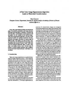
5. RESULTS Figure 2 depicts the results of the non-contextual labeling (sub-figure (b)) and of the Markovian labeling (sub-figure (c)) on the PEPPERS color image. As one can see, the objects are correctly segmented. We have also applied the method we propose onto about a dozen of color images. Images and results from this paper, as well as other resources, can be fetched from the address: http://www.lrde.epita.fr/download/. We have obtained remarkable results with our method on several other images. With the classical HOUSE image, an easy image for the classification in the color space, the cluster detection is performed as expected. On the TIFFANY image, the color cluster corresponding to the lips has been properly identified despite the fact that this cluster corresponds to very few pixels in the original image. On the PILLS image, the color pills have highly specular surfaces but that does not affect the segmentation correctness. On the COMP 10 image (digitalization of the painting “Composition X” by Kandinsky), the numerous colors used to depict the objects in that painting have led to different classes although the corresponding clusters are very close to each other in the RGB space. In the LAUVES image (digitalization of the painting “The Garden at Les Lauves” by C´ezanne), the segmentation suits well to the shape of the various bold blocks of color in that painting. We have noticed the same good results with the TUNISIAN image (from the “Southern Tunisian Gardens” by Klee), which however is a watercolor painting with many gradations. 6. CONCLUSION In this paper, we have presented an automatic classification method based on mathematical morphology and dedicated to color images. We have brought to the fore that the connected watershed algorithm can serve as a classifier, which is an uncommon task for that operator. In particular, we have shown that it provides very good results even in the case of color images that are difficult to segment. However, a main drawback of our method remains to be solved: it is both memory and time consuming.

7. REFERENCES [1] W.H. Cho, S.Y. Park, and J.H. Park, “Segmentation of color image using deterministic annealing EM,” in Proc. of the IEEE Intl. Conf. on Pattern Recognition, Barcelona, Spain, Sep. 2000, vol. 3, pp. 646–649. [2] D. Comaniciu and P. Meer, “Robust analysis of feature spaces: Color image segmentation,” in Proc. of IEEE Conf. on Computer Vision and Pattern Recognition, San Juan, Puerto Rico, June 1997, pp. 750–755. [3] P. Soille, Morphological Image Analysis – Principles and Applications, Springer-Verlag, 1999. [4] A. Bieniek and A. Moga, “An efficient watershed algorithm based on connected components,” Pattern Recognition, vol. 33, no. 6, pp. 907–916, 2000.

(a) original color image

[5] L. Vincent and P. Soille, “Watersheds in digital spaces: an efficient algorithm based on immersion simulations,” IEEE Trans. on PAMI, vol. 13, no. 6, pp. 583– 598, 1991. [6] K. Saarinen, “Color image segmentation by a watershed algorithm and region adjacency graph processing,” in Proc. of IEEE Intl. Conf. on Image Processing, Austin, TX, USA, Nov. 1994, vol. 3, pp. 1021–1025. [7] T. G´eraud, J.-F. Mangin, I. Bloch, and H. Maˆıtre, “Segmenting internal structures in 3D MR images of the brain by Markovian relaxation on a watershed based adjacency graph,” in Proc. of the IEEE Intl. Conf. on Image Processing, Washington DC, USA, 1995, vol. 3, pp. 548–551.

(b) non-contextual labeling (S)

[8] J.-G. Postaire, R.D. Zhang, and C. Lecocq-Botte, “Cluster analysis by binary morphology,” IEEE Trans. on PAMI, vol. 15, no. 2, pp. 170–180, 1993. [9] R.D. Zhang and J.-G. Postaire, “Convexity dependent morphological transformations for mode detection in cluster analysis,” Pattern Recognition, vol. 27, no. 1, pp. 135–148, 1994. [10] S.H. Park, I.D. Yun, and S.U. Lee, “Color image segmentation based on 3-D clustering: Morphological approach,” Pattern Recognition, vol. 31, no. 8, pp. 1061– 1076, 1998. [11] P. Soille, “Morphological partitioning of multispectral images,” Journal of Electronic Imaging, vol. 5, no. 3, pp. 252–265, 1996. [12] J. Besag, “On the statistical analysis of dirty pictures,” Journal of the Royal Statistical Society, vol. 48, no. 3, pp. 259–302, 1986.

(c) Markovian segmentation (S m ) Fig. 2. Results obtained on the PEPPERS image.