Combining SPIN with ns-2 for protocol optimization - SpinRoot

Combining SPIN with ns-2 for protocol optimization? Pedro Merino1 and Alberto Salmer´on1 University of M´ alaga, Campus de Teatinos, 29071, M´ alaga, Spain {pedro,salmeron}@lcc.uma.es

Abstract. In the field of communication networks, protocol engineers usually employ several tools focused on specific kinds of analysis, such as performance or correctness. This paper presents an approach to integrate the analysis capabilities of the Spin model checker and the ns-2 network simulator into a single framework. In particular, we use the verification capabilities of Spin to control the execution of ns-2. The traffic-oriented model of the protocols is managed by ns-2, while SPIN automatically generates the most suitable configurations of each ns-2 run in order to meet some designer requirements. These requirements are specified with assertions and with an annotated temporal logic that can be translated into Spin s B¨ uchi automata. Spin verification algorithms help us to automatically discard those ns-2 configurations and simulations that do not satisfy the expected requirements. With this approach we can automatically obtain the suitable values of parameters like buffer size, timeout to retransmit, window size, packet size, etc., to optimize a protocol implementation for a good performance in a given scenario. The paper presents the architecture for this integration, the modified temporal logic and its successful application to obtain optimized versions of protocols for videostreaming in wireless networks.

1

Introduction

The successful deployment of new networking systems, like those involving mobile phones, depends on the use of the proper techniques to produce robust and efficient implementation of communication protocols. In the design phase it is necessary to check that the protocol is free of negative behaviors like deadlock, its ability to handle situations such as connection loss or traffic congestion or its capacity to meet an expected throughput. Analysis of these concerns can be done by computer-aided simulations based on models of the protocols or by gathering data from real implementations. Aspects like correctness and reliability can be effectively checked with model checkers like Spin[1] (actually, this was the original focus of the tool). Performance analysis can be done by monitoring the network; however, large scale analysis is mostly performed with network simulators, like ns-2 [2]. ?

This work has been partially funded by the Government of Andalusia under grant P07-TIC3131.

A major problem in performing a full model based analysis is that the formal methods community and the communication protocols community usually employ different bases to describe the protocols and the desired properties or behavior and to perform the analysis. Model checking based analysis normally considers extended communicated finite state machines as models, temporal logic to represent properties and reachability analysis to check correctness and reliability. The critical part usually is the correct abstraction level to make the specification verifiable with standard computer resources. Network simulators usually consider probability distributions to model the source of data or the behavior of transmission media, algorithms to describe the processing of the messages and scripts to describe the simulation scenarios. The key issue to obtain good results is the choice of the initial configuration to start simulation, defining values for packet size, buffer size, window size, timeouts, etc. Some works geared to the integration of both types of analysis consist in extending model checker languages with performance oriented features, like time and probability[3][4][5]. Other approaches consider metamorphosing and model transformation to use the right tool from the same initial description [6]. In this paper, we propose a new method to combine model checkers and networks simulators to take advantages of both tools without the need to rework on the modelling languages. The combination works as follows. The model of the protocol is the one oriented to performance analysis with the network simulator, which produces a running for a given scenario and an initial configuration. The model checker makes the network simulator generate all the simulations by generating all possible initial configurations to be analysed. However, we do not execute all the simulations completely; that would take days or weeks for realistic protocols. We allow the protocol designer to specify temporal logic formulas that describe desired evolutions, considering performance as the key objective. The satisfaction of these formulas produces the desired initial configurations and acts as a powerful mechanism to discard unproductive simulations of the networks simulator. The resulting framework can be used to automatically tune a protocol to give the desirable performance in a specific scenario. We have implemented the proposal combining the model checker Spin and the network simulator ns-2 and demonstrated its utility in the tuning of parameters to optimize video download in wireless environments. The paper presents novelties compared with related works. The workflow automation tool ANSWER[7] presents a similar approach to our work. Its main objective is to ease the burden of performing exhaustive simulations with several configurable variables and its posterior analysis. An XML configuration file is used to specify the variables that must be combined to generate the set of different scenarios and its valid values, the metrics to check and other options. Configuration variables can be nested, which is useful to maintain the coherence of variables that have dependences between them. This reduces the probability of incurring in errors when defining and performing such simulation scenarios. The launcher module of ANSWER generates the set of scenarios declared on the XML file, performs the corresponding simulations, and stores the output metrics

in an organized way, to help correlate the scenario with its metrics. The drawer module is a web application that can plot diagrams for a single metric among a series of selected simulation scenarios. This tool uses a previous framework for data collection and statistical analysis[8]. This is complementary to our tool, since we rely on the model designer to provide the relevant metrics. This framework also provides support for gathering statistics by performing a series of independent runs of the same scenario, e.g. until a confidence interval is reached. Our tool does not support this kind of statistical analysis, and is oriented to checking properties in single runs of a large set of simulation scenarios. The rest of the paper is organized as follows: network simulators and protocols for video downloads are introduced in Sect. 2. The ideas behind our integrated approach are discussed in Sect. 3. The specification of properties for controlling the simulations is covered in Sect. 4. A study regarding video download over TCP is shown in Sect. 5. Section 6 discusses some implementation details of our prototype tool. Finally, Sect. 7 summarizes our conclusions and points to future work.

2 2.1

Background Network Simulators

One of the most used tools when evaluating network protocols and scenarios are network simulators. Network simulators can help profile the performance of a protocol during the design phase, or evaluate several alternatives in a given scenario when deploying a networked system. These tools are built to be able to cope with large scenarios comprising real-world network elements such as routers, nodes with their own TCP/IP stacks and applications making use of these resources. ns-2 [2] is an extensible network simulator, used by a large community as their tool of choice to test new protocols or analyze network scenarios. ns-2 is an eventoriented simulation, i.e. it has a scheduler that maintains a list of future events and advances time according to these events. It provides a number of protocols and network elements that can be used to simulate both wired and wireless networks. For instance, ns-2 comes with several TCP and UDP implementations as well as routing protocols that can be used to create new scenarios easily. ns-2 has been developed using C++ and OTcl (an object-oriented variant of Tcl). This makes the simulator easy to use and adapt through dynamic scripts, while also being efficient for large simulations. OTcl is mostly used for declaring network topologies and simulation scenarios, and for attaching actions to certain hooks, e.g. logging the reception of a packet, while protocols and other network elements are developed in C++. Both sides are not independent and can communicate to send commands, invoke hook procedures, etc. ns-3 [9] is being developed as an eventual replacement for ns-2, written from scratch in C++ and Python. However, ns-3 has not yet matched all the fea-

tures offered by the previous version, and many scientific papers still use ns-2 to implement and analyze new protocols.

2.2

Video download over TCP

Multimedia is one of the key services of the Internet of late. Improvements on the bandwidth and quality of the connections has increased the demand of audio & video content, either streamed or downloaded. Many efforts have been directed towards defining appropriate protocols for multimedia streaming in real time. One such protocol is the RTP (Real-time Transport Protocol), usually over UDP. The datagram-oriented nature of UDP allows frames to be sent separately without confirmation from the receiver. Lost frames may produce errors in the playback, but the real-time nature of multimedia streaming discourages retransmissions. However, one of the most successful Internet video services of recent years, YouTube1 , is built around downloading the content over a simple TCP connection, using HTTP as with any other web content. Since the video content is not broadcast in real-time, there is less pressure on the transport protocol, which does not have to deal with the mentioned challenges. However, a key point of these video services is that playing can start before downloading the whole video. After a small portion of the video has been downloaded and buffered, playing starts while the video is still being downloaded in the background. This means that the video can stall if the buffer runs out while playing, e.g. if the data rate demanded for the video playback is significantly larger than the download rate. One solution is to use an adaptive initial buffer size instead of a fixed one, so that if the data connection is slow more video will be buffered before starting the playback. Figure 1 shows a high level model of video playback over TCP, which we will use as a running example through the rest of the paper. The client and server are regular web clients which use the HTTP protocol over TCP to download web content, like the video being played. The client has a playout buffer where the video being downloaded is stored. The playback process will retrieve the video frames from this buffer. To simplify the model a constant frame size and rate is assumed. We also assume the server outputs the video at a constant bit rate, which is smaller than the bandwidth capacity of the link between the client and the server. Figure 2 shows a simple state diagram for the client. The key element in the client is the playout buffer. When the buffer is empty, e.g. right at the start, the playing is stopped. As soon as the first video frame is received the client is said to be buffering. However, playing cannot start until the playout buffer reaches a certain threshold. If during playback the buffer empties, e.g. because the playing rate is significantly higher than the receiving rate, the playing stops and buffering must happen again. When the video is completely received from 1

http://www.youtube.com

Fig. 1. Overview of video download over TCP

the server it is guaranteed that it will not stop playing again, so we consider this the final state.

Fig. 2. State diagram of the client

There has also been an increment in the demand of Internet services, including multimedia, from mobile devices such as mobile phones or laptops connected through mobile telephony networks. These devices have their own set of challenges which stem from the fact that the network link has less bandwidth and is more prone to network errors or disconnections, e.g. when moving from one cell to another, or when entering a zone with bad coverage. Although the lower layers of the mobile protocol stack are prepared to deal with these kind of issues, some of these still affect the upper transport layers, e.g. IP and TCP. For instance, a short disconnection time may be interpreted by TCP as a sign of congestion and thus activate the congestion control mechanism. This is because TCP was conceived for wired computer networks, where the impact of errors in the channel is considered negligible and congestions are much more frequent. This has led to the appearance of some TCP variants that try to address some of the key challenges that mobility poses. One of these variants is FreezeTCP[10], which improves the response against predictable disconnection drops. In the event of an impending disconnection the client warns the server in advance in order to “freeze” the connection. When connection is reestablished the client notifies the server and the connection is “unfrozen”, i.e. it returns to the same state as before the disconnection. In standard TCP the client sends probes to poll the connection, slowing down with each failed attempt. In addition, after the reconnection is detected, there is a slow start phase during which the connection

is underutilized. One of the advantages of Freeze-TCP over other TCP variants is that it uses existing TCP mechanisms and only requires modifying the client. Still, some information must be shared between layers so TCP can detect an impending disconnection. However, while Freeze-TCP can cope with long or frequent disconnections, it is not suitable for managing connections with a high error rate. We will use a mobile scenario for our case studies, thus Fig. 1 shows a mobile phone as the video client connected to the server through a link that may drop every few seconds. This scenario can be described as a ns-2 model such as the extract on Fig. 3, which shows the network elements, the protocols and the applications which make use of this networking stack.

set node0 [ $ns node ] set node1 [ $ns node ] set set $ns $ns

tcpserver [ new Agent / TCP ] tcpsink [ new Agent / TCPSink ] attach-agent $node0 $tcpserver attach-agent $node1 $tcpsink

set tcpvideoserver [ new Application / Traffic / CBR ] set tcpvideoclient [ new Application / TCPVideo / Client ] $tcpvideoserver attach-agent $tcpserver $tcpvideoclient attach-agent $tcpsink $ns connect $tcpserver $tcpsink $n2 at 0 .0 " $tcpvideoserver start " Fig. 3. Extract of a ns-2 scenario definition for video downloading over TCP

3

Integration approach

In this section we describe the ideas and architecture behind our integration approach. The starting point is the specification of the protocol in a dual way, one view for ns-2 and a second view for Spin. Both views depend on the requirements of the actual scenario where the protocol should run and the additional constraints given by the designer. From these views, the main tasks are generating a series of simulation scenarios according to a specification, launching these simulations and searching for the ones that satisfy the given properties. The Spin model checker is used to drive the whole process, while ns-2 is used to run each generated scenario and provide information back to Spin in the form of measured variables. A high level workflow of this approach can be seen in Fig. 4. The protocols and other network elements can be configured to create a particular instance of a scenario. For instance, in keeping with the running example

Fig. 4. Overview of our integrated approach

outlined in the previous section, the link between the nodes can be set up with parameters such as bandwidth or delay, while the TCP segment size can be set on the server, as shown on Fig. 5. Spin can generate combinations of these variables automatically to test and compare different configurations of the protocols in a given scenario.

$ns duplex-link $node0 $node1 $link_bw $link_delay DropTail $tcp_ set packetSize_ $segment_size $tcp_ set window_ $max_tcp_window $server_ $server_ $client_ $client_ $client_

set set set set set

packetSize_ $segment_size rate_ $cbr_rate frame_rate_ $frame_rate frame_size_ $frame_size buffer_size_ $buffer_size Fig. 5. Configuring the elements of a ns-2 scenario

However, Spin is not directly aware of the implications of the selection of a particular configuration, it only knows about these values. The behavior of the protocols, the dynamics of the network, etc., is managed by ns-2, which uses this information to simulate the evolution of the system. To allow Spin to check the satisfiability of certain properties of interest to the simulation, ns-2 exposes some

of its internal state so that Spin can reason about it. Thus, each tool holds a different view of the system derived from the initial specification and constraints set by the designer. Regarding the state space exploration, the resulting structure resembles a tree at the beginning and after a certain depth is made of linear branches, as can be seen on Fig. 6. The generation of the possible initial configurations for the simulations creates a tree-like space state. At each step a configuration variable is given a value, and there are as many branches from a step as possible values. On the other hand, we consider each simulation run to be linear, i.e. given an initial configuration, the ns-2 simulator will keep running forward without creating any alternative that may be backtracked to. Thus, each simulation run produced by ns-2 is represented in Spin as a single branch with several states, one for each valuation of the measurement variables that is shared from ns-2 to Spin. In the following section, we give a more rigorous description of the state space.

Fig. 6. Overview of the space state generated by Spin from the ns-2 simulations

4

Temporal properties for controlling simulations

Given a series of variables that can be set in a simulation scenario, running all possible scenarios that can be generated from those variables may be too time consuming to be of any use. However, most of the time these simulations are performed in order to check certain properties, e.g. if the protocol under study meets certain performance objectives. This information can be used to guide the simulation generation and execution process, instead of performing a brute-force approach by running every possible scenario completely.

There are several kinds of properties that may be useful in order to control the simulations in this sense, usually setting an objective that they have to meet or a constraint to discard a set of unwanted simulations. In addition to guiding the selection of initial configurations to simulate, setting objectives may help in stopping simulations early and thus reducing the time and number of states needed. These properties may be expressed over the configuration variables or over the evolution of the measured variables during a simulation. In this section these properties are described and examples are given based on the running example of Sect. 2.2. 4.1

Extending LTL

State space. We define CC as the finite ordered sequence of initial simulation configurations Ci : 0 ≤ i ≤ n. Each initial configuration Ci is a valuation of the configuration variables cvar, Ci : cvar → domain(cvar), with Ci 6= Cj for every i, j ∈ (0, n), i 6= j, being n the cardinality of CC. The sequence of states traversed during a simulation with initial configuration Ci is run(Ci ) = si0 , si1 , si2 . . ., with run(Ci )0 = si0 . Propositions and variables. As variables we may use both the configuration variables cvar that determine the initial configuration of a simulation and the variables mvar measured during a simulation run. Let var = cvar ∪ mvar be the set of variables, and domain(v) the domain of variable v ∈ var. We assume that variables are in standard domains such as boolean, integer and real. A proposition is either a boolean variable, or is constructed using the equality or comparison operators of each domain, e.g = and 250ms)) We can combine these properties to express more complex objectives. For instance, if we are looking for the first simulation in which the video is completely downloaded but we do not want extreme corner cases, we can combine f1 and f3 : f4 = F IRST ( 3(status = Downloaded) ∧!2(bandwidth < 64Kbps ∧ delay > 250ms)) 4.3

Further optimizations

The Spin view of the protocol could also provide support for a specific kind of state space exploration optimization. This optimization takes advantage of the additional knowledge a designer may have over the relationships between initial configurations and their outcomes. If a certain configuration mets (or fails to meet) an objective, it can be deduced that certain similar configurations will have the same outcome, and thus do not have to be run. Let R./ ⊆ Ci × Cj × ltl, ./ ::= |= | 6|=, be a relationship defined using propositions over the variables of Ci and Cj . Let v ∈ cvar and vi = Ci (v), R is defined as boolean formula using propositions of the form defined in Sect. 4.1 between the variables of Ci and Cj and the values of their domains, e.g. vi > vj or vi = 10. Additional knowledge derived from a relationship R./ is defined as: Ci |= ltl ⇒ Cj |= ltl

iff i < j and (Ci , Cj , ltl) ∈ R|=

Ci 6|= ltl ⇒ Cj 6|= ltl

iff i < j and (Ci , Cj , ltl) ∈ R6|=

We extend the satisfiability operator |= to support the additional knowledge expressed in a relationship R./ :  true if ∃j : j < i, (Cj , Ci , ltl) ∈ R|= Ci |=R|= ltl = Ci |= ltl if @j : j < i, (Cj , Ci , ltl) ∈ R|=  true if ∃j : j < i, (Cj , Ci , ltl) ∈ R6|= Ci 6|=R|= ltl = Ci 6|= ltl if @j : j < i, (Cj , Ci , ltl) ∈ R6|= For instance, we can use this to reduce the state space that needs to be explored while evaluating the formula f1 in Sect. 4.2 thanks to the additional knowledge the designer has on the system. One of the configuration parameters is the playout buffer size, called buffer . We know for sure that if an initial configuration meets the objective declared on f1 , increasing the size of the playout buffer in the client will not affect the rest of the system, and thus the objective will be met as well. We can express this additional knowledge with the following relationship:

|=

(Ci , Cj , f1 ) ∈ Rbuffer if buffer i < buffer j and vi = vj for every v ∈ cvar, v 6= buffer The pairs of initial configurations in this relationship are those which have the same initial configuration but only differ on their buffer variable, which is greater on Cj . By enriching the evaluation of formula f1 with the additional knowledge provided by this relationship, we guarantee the same results, while reducing the space state at the same time.

5

Case Study: downloading YouTube videos

To test our integrated approach we choose as our case study an application that downloads and streams a video over TCP to a mobile TCP client, e.g a mobile phone, as described in Sect. 2.2. This is the same schema that a YouTube video follows when it is transmitted over HTTP. However, for the sake of simplicity we ignore the impact of the HTTP header overload, which is about a kilobyte compared with the several megabytes of video content. This scenario is similar to the one studied in [11], which also uses ns-2 to simulate a set of configurations. The scenario comprises two nodes connected through a link with drops, which drops periodically for a given amount of time. Each node has a TCP agent with an application on top: one node has an Application/TCPVideo/Client instance while the other has an Application/Traffic/CBR instance. The first application was developed in C++ to simulate both the reception of video using TCP and the playback engine at the client. The client has a playout buffer (a simple counter) in which all TCP segments are placed upon arrival. This buffer is read 30 times per second to simulate the fetching of each video frame by the playback engine at 30 fps. The client also makes its state (see state diagram on Fig. 2) available through an instance variable. The scenario itself is defined using regular ns-2 commands suchs as the extracts seen in Figs. 3 and 5. The configuration variables and their possible values are defined in Table 1. These variables are related to both the environment, e.g. the duration of uptime and downtime periods of the link, and the elements of the protocol stack, e.g. segment size and maximum window size for TCP. The combination of the different valuations of each variable constitutes the set of initial configurations that we want to analyze. We are interested in those initial configurations in which the video can be downloaded fully without stopping for rebuffering once playing has started. This objective is a combination of the ones in formulas f1 and f2 in Sect. 4.2. The first part of the formula states that we want the initial configurations to reach the Downloaded state, e.g. the video has been completely downloaded. At the same time, the second part of the formula prevents any simulation where the video stops during playback from being returned. This objective is expressed with the following formula:

Table 1. Configuration variables and their possible values for the case study Variable Link uptime Link downtime Link delay Link bandwidth Max. TCP window TCP segment size Playout buffer length Freeze warning

Values 20 s 100 ms – 1 s 100 ms 384 Kb 5 KB – 10 KB 0.1 KB – 0.3 KB 1 s – 10 s 0.2 – 2.0 RTTs in advance

objective = ALL( 3(status = Downloaded) ∧!3(status = Playing ∧ 3(status = Stopped))) We can optimize our search further and add the additional knowledge declared in the sample relationship at the end of Sect. 4.3. This relationship declares that increasing the playout buffer size of an initial configuration that already satisfied the formula above guarantees that the new initial configuration will satisfy the formula as well: |=

(Ci , Cj , objective) ∈ R if buffer i < buffer j buffer and vi = vj for every v ∈ cvar, v 6= buffer The experiments were performed on an Intel Core i7 920 2.6GHz with 4GB of RAM running Ubuntu Linux. We used Spin version 5.2.4 (running on a single core) and ns-2 version 2.33. Table 5 shows some measures taken from the experiments. The first column shows the results of the experiments when neither objectives nor optimization are used, the second shows the results when the objective formula is set, and the third row gives the results when additional knowledge is also used. The first row contains the number of states analyzed by Spin. The second and third rows give the number of simulations that had to be run to find out if they satisfied the given objective, and the number of simulations that did not have to be run because their outcome could be deduced |= from the additional knowledge expressed in R , respectively. The fourth buffer row shows how many simulation runs meet the objective. The fifth row gives the number of simulations that were stopped early thanks to the second part of the objective formula. Finally, the sixth row shows the total time spent on each experiment. These results show that there is a notable improvement in the experiment running time when properties are used. In addition to only returning the desired initial configurations, setting objectives helps stopping simulations early and thus reduces the space state that needs to be explored. In this case, the state space was about 5 times smaller when properties were used. Using additional

Table 2. Results for the experiments using regular TCP, depending on the properties used Properties Number of Spin states Simulations run Simulations not run Objective met Rejected by objective Total time

|=

None objective objective and R buffer 85367 17468 15860 1100 1100 966 – – 134 – 169 169 – 931 931 351 s 146 s 122 s

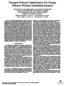
knowledge also reduces the number of simulations that must be run because their outcomes can be inferred. This can be seen on the third row of the third column, where 134 simulations (of the 1100 total) did not have to be run to check the satisfiability of the objective. Figure 7 shows the influence of the configuration variables on the evaluation of the objective. The graph on the left plots the maximum TCP window size against the playout buffer length, for several values of TCP segment size. As the window size increases video playback can start sooner, as the playout buffer fills more quickly. The graph on the right shows the converse relationship, plotting the TCP segment size against the playout buffer length. From that graph it can be deduced that using bigger segments means less video must be buffered before playback can start. From both graphs it can be seen that no simulation with a playout buffer of less than 10 seconds satisfies the objective. This is caused by a combination of the video length and the disconnections during the transmission, i.e. the sum of the duration of the disconnections suffered during the video transmission is long enough so that, combined with the slow start phase of TCP, it is almost impossible to overcome this gap with less than 10 seconds of margin. As we mentioned in Sect. 2.2, applications in mobile environments have to face new challenges such as fluctuating network conditions. One solution to improve the performance in these environments is to use a transport protocol designed for mobility such as Freeze-TCP[10]. In our analysis we will use an existing ns-2 model of the protocol available from [12]. Freeze-TCP depends on the ability of the mobile device to predict impending network disconnections. This notification should come from the physical layer, as it can monitorize the quality of the received signal. We simulate these notifications and issue them automatically a given amount of time before the disconnection happens. The time of when the freeze warning must be sent is also a sensible parameter of Freeze-TCP, and as such we have added it to the configuration variables to optimize it. Figure 8 shows the influence of the freeze warning on the performance of this experiment. Freeze warnings are measured in RTTs (round-trip times) and, according to [10], ideally they should be sent 1 RTT before the disconnection. However, as can be seen on the figure, this also depends on the duration of the link downtime periods. A smaller downtime means that the warning can be sent

TCP segment size = 170 bytes

Max TCP window size = 7,5KB

TCP segment size = 238 bytes

Max TCP window size = 9,0KB Max TCP window size = 10,0KB 310

TCP segment size (bytes)

Max TCP window size (bytes)

TCP segment size = 306 bytes 10500

9500

8500

7500

270 230 190 150

0

5

10

15

20

0

5

Buffer length (s)

10

15

20

Buffer length (s)

Fig. 7. Influence of maximum TCP window size and TCP segment size in the first experiment

some time before the disconnection really happens, putting less pressure on the prediction algorithm. The bigger the downtime, the less important is to predict it precisely, as the duration of the disconnection is considerably larger than the idle time wasted freezing the connection earlier. Comparing this graph with the ones in Fig. 7 it can be seen that the freeze mechanism allows a smaller playout buffer to be used, as the effect of the disconnections is partially mitigated.

6

Implementation details

Our prototype implementation2 follows the architecture described in Sect. 3. This architecture requires the integration of Spin with an external tool (ns-2), which is possible thanks to the ability to use embedded C code in Promela. Spin is responsible for generating all the possible initial configurations and for running the corresponding simulations on ns-2. A new ns-2 process is spawned for each simulation, and communication is handled through input redirection and sockets. Spin first loads the scenario in ns-2 and sets up the configuration variables, the during the simulation the ns-2 process reports back to Spin the measured values of the variables of interest. To control this process from Spin we have defined a Promela template that must be instantiated for the given scenario and constraints. The main reason for this is that Spin does not allow state variables (which will store the configuration and measure variables) to be declared dynamically. An extract of the template is shown in Fig. 9. The prototype also maintains a database with the initial 2

The prototype tool and the case study http://www.gisum.uma.es/tools/spinns2.

will

be

made

available

at

2

Freeze warning (RTTs)

1,5

Downtime = 100ms

1

Downtime = 300ms Downtime = 600ms Downtime = 1000ms 0,5

0

0

2

4

6

8

10

Buffer length (s)

Fig. 8. Influence of freeze warning in the second experiment

configurations and their corresponding results, which is used to check properties regarding additional knowledge over the initial configurations as defined in Sect. 4.3. On the ns-2 side we have implemented two classes in C++ to prepare the simulation environment and handle the communication with Spin, respectively, which are instantiated when ns-2 is launched. The network model under analysis must make use of the environment provided by these classes to expose the measure variables of interest to Spin.

7

Conclusions and Future Work

We have presented an approach to integrate on-the-fly model checking with network simulators. This proposal has implemented in a prototype tool that takes advantage of the Spin model checker and the ns-2 network simulator to perform large scale property-driven simulation of network scenarios. This tool has been proven useful for generating scenarios that verify a certain performance property of interest, while also terminating unpromising simulations early to avoid wasting simulation time. This is especially useful when the number of different possible scenarios is quite large and the simulation time of each run makes it impractical to perform each one of them in its entirety. The work can be extended in several ways. The first one is to increase the information directly managed by Spin. Apart from the temporal formulas, we plan to also describe in Promela part of the behavior of the protocol to increase efficiency and the ability to check more properties.

/* [ never_claim ] */ bool running = false ; c_state " double time " " Global " " -1.0 " /* [ c_state ] */ c_code { short wasRunning = 0; } /* [ ge n e r a t e _ c o n f i g _ i n l i n e s ] */ inline generateConfig () { /* [ generate_config ] */ } inline runSimulation () { c_code { if ( wasRunning == 1) { t e r m i n a t e P r e v i ou s B r a n c h () ; wasRunning = 0; now . running = 0; } startSimulation () ; wasRunning = 1; now . running = 1; }; do :: ( running ) -> c_code { ss_getM easure Time ( " time " , & now . time ) == -1) ; if ( now . time < 0) { Printf ( " Simulation finished at % fs \ n " , now . time * -1) ; now . running = 0; } else { /* [ read_measures ] */ } }; :: (! running ) -> break od ; c_code { finishSimulation () ; wasRunning = 0; } } init { c_code { s s _ l a u n c h S er v e rS o c ke t () ; }; generateConfig () ; runSimulation () } Fig. 9. Extract of the Promela template for generating and controlling simulations. Comments of the form /*[label]*/ are placeholders.

Regarding the tool, we are also looking into improving its usability by developing a GUI front-end. Another direction in which the tool can be improved in both usability and expressiveness is allowing the use of different property specification languages. For instance, currently only one LTL formula at the same time is supported, which may me reduce the combinations of objectives that can be expressed. New property specification languages may be supported for different purposes, e.g. a quality-of-service oriented language or even graphical notations like SDL’s message sequence charts or UML’s sequence diagrams. Finally, the core of the tool can also be extended in a number of ways. The multi-core capabilities of Spin may be used to launch several simulations at once, thus taking advantage of modern multi-core CPUs. Other network simulators could also be supported by the tool, such as ns-3, or OMNeT++, although the core algorithm is generic and reusable for any simulator.

References 1. Holzmann, G.J.: The SPIN Model Checker: Primer and Reference Manual. Addison-Wesley Professional (September 2003) 2. The Network Simulator - ns-2: http://www.isi.edu/nsnam/ns/. (February 2010) 3. Yovine, S.: KRONOS: A Verification Tool for Real-Time Systems. STTT 1(1-2) (1997) 4. Larsen, K., Pettersson, P., Yi, W.: UPPAAL in a Nutshell. International Journal on Software Tools for Technology Transfer 1(1-2) (1997) 5. Kwiatkowska, M., Norman, G., Parker, D.: Prism: Probabilistic model checking for performance and reliability analysis. ACM SIGMETRICS Performance Evaluation Review 36(4) (2009) 40–45 6. Gallardo, M.M., Mart´ınez, J., Merino, P., Rodriguez, G.: Integration of reliability of performance analyses for active network services. Electronic Notes in Theoretical Computer Science 133 (December 2005) 217–236 7. Andreozzi, M.M., Stea, G., Vallati, C.: A framework for large-scale simulations and output result analysis with ns-2. In: Simutools ’09: Proceedings of the 2nd International Conference on Simulation Tools and Techniques, ICST, Brussels, Belgium, Belgium, ICST (Institute for Computer Sciences, Social-Informatics and Telecommunications Engineering) (2009) 1–7 8. Cicconetti, C., Mingozzi, E., Stea, G.: An integrated framework for enabling effective data collection and statistical analysis with ns-2. In: WNS2 ’06: Proceeding from the 2006 workshop on ns-2: the IP network simulator, New York, NY, USA, ACM (2006) 11 9. The ns-3 network simulator: http://www.nsnam.org/. (April 2010) 10. Goff, T., Moronski, J., Phatak, D., Gupta, V.: Freeze-tcp: a true end-to-end tcp enhancement mechanism for mobile environments. In: INFOCOM 2000. Nineteenth Annual Joint Conference of the IEEE Computer and Communications Societies. Proceedings. IEEE. Volume 3. (Mar 2000) 1537–1545 11. Shen, X., Wonfor, A., Penty, R., White, I.: Receiver playout buffer requirement for tcp video streaming in the presence of burst packet drops. In: London Communications Symposium 2009. (2009) 12. NICTA: Freeze-tcp (ns-2 and linux implementations): http://www.nicta.com.au/people/mehanio/freezetcp. (July 2009)