Comparing backpropagation with a genetic algorithm ...

Omega 27 (1999) 679±684

www.elsevier.com/locate/orms

Comparing backpropagation with a genetic algorithm for neural network training Jatinder N.D. Gupta a,*, Randall S. Sexton b a Department of Management, Ball State University, Muncie, IN 47306, USA Computer Information Systems, Southwest Missouri State University, 901 South National Avenue, Spring®eld, MO 65804, USA

b

Received 1 April 1998; accepted 1 March 1999

Abstract This article shows that the use of a genetic algorithm can provide better results for training a feedforward neural network than the traditional techniques of backpropagation. Using a chaotic time series as an illustration, we directly compare the genetic algorithm and backpropagation for e€ectiveness, ease-of-use, and eciency for training neural networks. # 1999 Elsevier Science Ltd. All rights reserved. Keywords: Neural networks; Backpropagation; Genetic algorithm; Empirical results

1. Introduction Wong et al. [1] found that an overwhelming majority of studies using neural networks (NNs) rely on gradient techniques for network training, typically a variation of backpropagation (BP) developed by Werbos [2] and popularized by Rumelhart and McClelland [3]. However, as pointed out by Curry and Morgan [4], BP and the gradient techniques do not provide the best and fastest way to train neural networks. The computational results of Curry and Morgan [4] and Porto et al. [5] show that the use of the polytope algorithm and a simulated annealing method provide a viable alternative for training neural networks. Because NNs generate complex error surfaces with multiple local optima, even for simple functions being estimated, BP tends to become trapped in local solutions that are not global. Chaotic system problems, as used in this study, are

* Corresponding author. Tel.: +1-765-285-5301; fax: +1765-285-8024 E-mail address: [email protected] (J.N.D. Gupta)

inherently complex, thereby generating complex error surfaces when neural networks are applied. Since BP converges locally, the solutions found by this gradient technique are highly dependent on the initial random draw of weights. Although the limitations of gradient search techniques are well known, the use of such techniques has not been limited and has often resulted in inconsistent and unpredictable performance of the neural networks [4]. To overcome this local convergence problem for solving dicult non-linear optimization problems, a number of techniques have been developed. The most common of these are the evolutionary programming approaches, which include the genetic algorithm (GA) [5±8], direct optimization methods using a polytope algorithm [4], and global search techniques like simulated annealing (SA) [5]. While the use of GAs for neural network training has been shown to be generally noncompetitive with the best gradient learning methods [9], it has been shown that the binary coding scheme used in these GAs is neither necessary nor bene®cial [10,11]. Intuitively, such implementation limits the e€ectiveness of the GA since various GA oper-

0305-0483/99/$ - see front matter # 1999 Elsevier Science Ltd. All rights reserved. PII: S 0 3 0 5 - 0 4 8 3 ( 9 9 ) 0 0 0 2 7 - 4

680

J.N.D. Gupta, R.S. Sexton / Omega 27 (1999) 679±684

Fig. 1. Outline of the Genetic Algorithm.

ations (e.g., crossover and mutation) are incompatible with binary encoding. This incompatibility is further demonstrated by Sexton et al. [12]. In this article, we use chaotic time series to directly compare the performance of a genetic algorithm, as used by Dorsey et al. [13,14], with the BP algorithm. We develop a rigorous comparison between the GA and BP that includes di€erent variations of the BP algorithm, additional NN architectures, and additional BP con®gurations in order to give BP a greater chance to outperform the GA. The performance measures used for comparison are e€ectiveness, ease-of-use, and eciency as de®ned below: . E€ectiveness: refers to the accuracy of each algorithm in estimating the true functional form. The Root Mean Squared Error (RMSE) is used for a direct comparison as well as the Wilcoxon Matched Pairs Signed Ranks test to establish a statistical di€erence between the GA and BP solutions. . Ease-of-use: deals with the e€ort needed for ®nding optimal algorithm settings for each problem. . Eciency: is the CPU time taken by each algorithm for converging upon the best found solutions in training NNs. The rest of the article is organized as follows: Section 2 brie¯y describes the genetic algorithm as it was used in training the NNs. The chaotic time series function used in the comparison of BP and GA algorithms is brie¯y discussed in Section 3 while Section 4 describes the experimental design for this comparison. Section 5 provides the results of the comparison followed by ®nal remarks and conclusions in Section 6.

2. The genetic algorithm Unlike BP, the GA searches for global solutions and does not require the objective function to be di€erentiable. Since error surfaces for even simple problems can be quite complex with many local optima, the GA seems to be better suited for this type of search. The genetic algorithm searches from one population of points to another, focusing on the area of the best solution so far, while continuously sampling the total parameter space. Dorsey et al. [13,14] designed a Genetic Adaptive Neural Network Training (GANNT) algorithm and showed that the GA also works well for optimizing the NN. The GANNT algorithm is di€erent from other genetic search algorithms in that it uses real values instead of binary representations of the weights. This algorithm has been shown to outperform SA for NN training [15]. In this research, we adapt their genetic algorithm for training our NN. Fig. 1 illustrates a simple outline of the GA used in this study. 3. Chaotic time series Deterministic chaotic dynamic systems, such as the function used in this study, are of great interest to researchers because of their comparability to the chaotic behavior of economic and ®nancial data. Chaotic systems, as discussed in this research, are special types of system that are capable of exhibiting complex, often aperiodic, behavior in time. Recently there has been great interest in determining whether certain ®nancial and economic time series are better described by linear stochastic models or are appropriately characterized by deterministic chaos. In such time series, empirical

J.N.D. Gupta, R.S. Sexton / Omega 27 (1999) 679±684

research has been hampered in detecting the presence of chaos due to the apparent randomness of these types of data. While the irregularity of such variables as GNP, employment, interest rate, and exchange rates have generally been attributed to random ¯uctuations, the ability of even simple deterministic chaotic models to produce complex time paths that appear to be random has attracted attention as a possible alternative explanation [16]. Taking this into consideration, the signi®cance of accurately estimating such chaotic behavior is apparent. In this paper we show that the use of GA, rather than BP, for training the NNs increases the ability of the network to correctly map such behavior. The time series problem used in this study is drawn from Mackey and Glass [17] and is shown in Eq. (1) below: Yt ˆ Ytÿ1 ‡ 10:5‰f0:2Ytÿ5 =…1 ‡ Y 10 tÿ5 †g ÿ 0:1Ytÿ1 Š

…1†

This equation is of special interest in economics applications because it can generate a time series that is similar to ®nancial market data. Its apparent randomness makes this equation dicult to estimate and makes it a good choice for algorithm comparison. The initial ®ve values of the time series were generated by drawing random values from a uniform distribution from the range [0,1]. Two thousand exemplars were generated for this problem. Each exemplar or observation consisted of 5 lag variables and 1 output value. Although we know that only tÿ1 and tÿ5 were used in calculation of the function, this information is usually unknown in time series prediction. Therefore, we include all 5 lag variables in the model and let the NN discriminate the inputs that are useful from those that do not contribute to the model. The ®rst 100 exemplars were used to train the network, while the last 100 exemplars were used to test the solutions found. By skipping over 1800 exemplars in the time series, we can test the NN's ability to accurately map the underlying function of the time series.

681

One critical property of this deterministic chaos is its systematic sensitivity to initial conditions. Since even minute changes in the initial value can cause drastic changes in resulting data values, it is necessary to test if the NN is able to correctly map the underlying function when di€erent initial conditions are present. Although the ®rst test set only included values that were 1800 points in the future, these test exemplars were still generated from the initial 5 random points. Since deterministic chaos is sensitive to initial conditions, a second test set was generated that included 100 exemplars that were initialized with a di€erent set of 5 randomly drawn values.

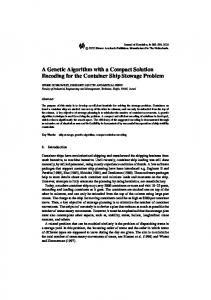
4. Experimental design Three NN architectures were used in this study. The architectures had three levels and only di€ered in the number of hidden nodes in the hidden node layer. These included networks with 2, 4, and 6 hidden nodes. Fig. 2 illustrates the architecture types for the NNs used in this study. While these di€erent architectures cannot be construed as optimal architectures for this problem, they are sucient to show the robustness of the GA for training the network as well as giving the BP algorithm the best chance possible to converge upon a good solution. The comparisons of the algorithms were based on the Root Mean Squared Error (RMSE) for in-sample and both out-of-sample test sets. 4.1. Training with backpropagation Commercial NN software packages were preliminarily evaluated in order to determine which package would give the best estimates for the given problem. The packages evaluated included Neural Works Professional II/Plus by NeuralWare1, BrainMaker by

Fig. 2. NN architectures.

682

J.N.D. Gupta, R.S. Sexton / Omega 27 (1999) 679±684

California Scienti®c, EXPO by Leading Markets Technologies and MATLAB by Math Works. Although performance was similar for all the programs, Neural Works Professional II/Plus seemed to give the best estimates and was chosen for the study. Since there has been much research on improving BP's performance, we used two variations of this algorithm. These were the Standard BP (SBP) algorithm and the Extended Delta-Bar-Delta (EDBD) variation [18], which were both included in Neural Works Professional II/Plus. Two parameters were manipulated in order to give SBP every opportunity to ®nd good solutions. These were the learning coecient ratio (LCR) and the momentum value. The LCR was used to incrementally decrease the size of the learning rate during training. The LCR was set at 10 levels that ranged from no decrease in learning rate to 0.9 decrease every 10,000 epochs. The momentum value was also set at 10 levels that ranged from 0.0 to 0.9, in 0.1 increments. The initial learning rate was set to 1.0. Since BP is highly dependent on the initial random draw of weights, 10 replications of each con®guration was implemented using di€erent random seeds, totaling 1000 networks for each architecture. The Extended Delta-Bar-Delta (EDBD) variation of BP attempts to escape local minima by automatically adjusting step sizes and momentum rates. Detailed information on this variation can be found in [19] and its enhancements in [18]. Since the EDBD has prespeci®ed learning schedules, there was no need to search for optimal learning rates or momentum values. These runs consisted of 10 replications for each network architecture, totaling 30 networks. 4.2. Training with the genetic algorithm The genetic algorithm trained for 100,000 epochs for 10 replications, only changing the random seed. This was also done for all three NN architectures, totaling 30 trained networks. Since the genetic algorithm automatically searches for the global solution, there was no need to manipulate any other factors.

5. Experimental results As mentioned earlier, comparisons were conducted on e€ectiveness, ease-of-use, and eciency. In this section, we describe these three comparisons and their respective results. 5.1. E€ectiveness In order to have a baseline comparison of how well the two variations of BP and the GA performed on estimating the function, linear regression (LR) was conducted using the in-sample data set. Taking the corresponding intercept and beta coecients, estimates were generated for both tests sets. Taking these estimates, RMSE values were then generated to compare with the RMSE values that were generated from SBP, EDBD, and NN estimates. Taking the best set of weights for each algorithm and architecture, estimates were then generated by running the in-sample and both test sets through the corresponding network. The RMSE was then calculated and used for comparisons for in-sample, test set 1 and test set 2. Table 1 shows the average RMSE values for each NN architecture and training method used. In comparison to regression analysis, it was found that, in all but one case, NNs found superior solutions. The one case in which regression outperformed the neural network was for the SBP variation for Test set 2. In comparison to the SBP and EDBD, not only did the GA ®nd better solutions for in-sample estimates but also found superior solutions for out-of-sample estimates. These comparisons also show that the GA captures the underlying function for the problem rather well. Table 2 illustrates the standard deviations of the RMSE values that were calculated from the 1000 replications for SBP, 10 replications for EDBD, and 10 replications for the GA for each of the three architectures. As can be seen from Table 2, the standard deviations of the RMSE from the GA are less than those of BP implying that GA solutions are better than those of BP. This intuitively makes sense because BP may converge upon local solutions. Depending where the search begins for BP, the solutions that result can

Table 1 Average RMSE comparisons Hidden node

6

4

2

Data sets

SBP

EDBD

GA

SBP

EBDB

GA

SBP

EDBD

GA

LR

In-sample Test set 1 Test set 2

0.079 0.135 0.166

0.124 0.183 0.218

0.041 0.050 0.050

0.054 0.096 0.147

0.125 0.174 0.243

0.043 0.055 0.066

0.259 0.348 1.108

0.423 0.478 0.439

0.145 0.164 0.172

0.573 0.639 0.640

J.N.D. Gupta, R.S. Sexton / Omega 27 (1999) 679±684

683

Table 2 RMSE Standard Deviations and mean CPU time Hidden nodes

6

4

2

Algorithm

SBP

EDBD

GA

SBP

EBDB

GA

SBP

EDBD

GA

Std. Dev. Mean CPU time

0.21 611.2

0.012 623.8

0.007 329.3

0.024 570.3

0.023 583.2

0.010 245.1

0.077 497.9

0.089 532.1

0.013 134.4

vary on its e€ectiveness for ®nding the best solutions, while the GA searches globally with multiple starting points for each network. Table 2 also shows the average time for convergence for all algorithms and replications. All algorithms were run on a 200 MHz Pentium Pro machine using Windows NT 4.0 operating system. Table 3 illustrates the best architectures or number of hidden nodes that found the best solutions for the in-sample, test set 1, and test set 2 data. It is interesting to note that the EDBD variation of BP found its best in-sample solution with an architecture of 6 hidden nodes but its corresponding estimates for the test set 1 was inferior to its best solution that included 4 hidden nodes. This corresponds with ®nding local vs global solutions. A local solution might perform well for in-sample but can perform erratically when applied to data which it has not seen. Since only three architectures were included in this study, we do not claim that any of these architectures are optimal for the given problem. Obviously, many more architectures are possible and the problem of determining optimal architectures is left for future research. A statistical comparison of in-sample, test set 1 and test set 2 was conducted using the Wilcoxon Matched Pairs Signed Ranks two-tailed P Signi®cance test. This test incorporates information about the magnitude of the di€erences as well as the direction of the di€erences between the pairs being tested. The best estimates for both BP and the GA were used for this test. The GA was found to be statistically superior to BP at 0.01 level of signi®cance. 5.2. Ease-of-use Since the correct parameter settings for BP are unknown, a wide variety of parameter settings were

tried to generate con®dence that optimal values were used. For each problem there were 100 di€erent con®gurations for the SBP variation. Each con®guration was then replicated 10 times using a di€erent random seed. Since the EDBD variation of BP had a pre-speci®ed learning schedule, there was no need to search for optimal parameter settings. However, in every case the SBP variation outperformed EDBD. For the EDBD variation, 10 replications were conducted that only changed the initial random starting point. BP solutions have also been shown to be dependent on the number of hidden nodes included in the network. In this experiment, we used three di€erent architectures including networks with 6, 4 and 2 hidden nodes. Combining all con®gurations and architectures, SBP algorithm had a total of 3000 opportunities for ®nding the best solution. Since the GA did not have to search for optimal con®gurations, this algorithm only had a total of 30 opportunities, including 10 replications with di€erent random seeds for each of the three architectures. Since there was no need to search for optimal parameter con®gurations for the GA and SBP outperformed EDBD, this algorithm was much easier to use. 5.3. Eciency The genetic algorithm found these superior solutions with fewer epochs. The BP algorithm terminated training once there were 100,000 epochs, over the initial 1,000,000 training cycle, without a reduction in error (error was checked every 10,000 epochs). For both BP algorithms, the training only terminated when errors ceased to decrease, as opposed to the GA, which terminated after the user-set 100,000 epochs. Although the GA was terminated before fully converging upon the ®nal solution, the training conducted for each problem was more than adequate to show superior sol-

Table 3 Best architectures for the GA and BP (hidden nodes) Hidden nodes

In-sample

Test set 1

Test set 2

Data sets

SBP

EDBD

GA

SDP

EDBD

GA

SBP

EDBD

GA

In-sample

4

6

6

4

4

6

4

6

6

684

J.N.D. Gupta, R.S. Sexton / Omega 27 (1999) 679±684

utions over BP. An even better measurement of eciency is the amount of average CPU time for each network. As can be seen in Table 2, the average CPU time for the GA was less than that for SBP and EDBD. 6. Conclusion This paper compared the use of backpropagation and genetic algorithms for optimizing arti®cial neural networks. For this chaotic time series problem, our empirical results show that the GA is superior to BP in e€ectiveness, ease-of-use and eciency in training NNs. Although the GA trained fewer networks, it was found to provide a statistically superior solution over BP. Since the GA did not need to ®nd optimal parameter settings, its ease-of-use was much greater than BP. This algorithm also found superior solution in less time, which is a major concern in NN research. Although BP is by far the most popular method of optimization for NNs, it is apparent from this research that a genetic algorithm may be more suitable for training the NNs. Even though this study only includes one function for comparison, it can be seen that the problem of local convergence will undoubtedly a€ect a wide variety of unknown functions that can be estimated using neural networks. By using a global search technique, such as the GA, for neural network training, many if not all problems associated with BP can be overcome. Several issues are worthy of future investigations. First, a comprehensive study to compare the performance of genetic algorithms and gradient search techniques through the use of other complex functions and real data from the complex areas such as economics and ®nance will be useful. Second, research studies to determine an optimal NN architecture to obtain the best results in the training of a given neural network will be interesting and worthwhile. Finally, the development and testing of hybrid algorithms, that use a combination of GA, BP, and other metaheuristics like Tabu Search to enhance the e€ectiveness and eciency of training arti®cial neural networks is both desirable and perhaps necessary. References [1] Wong BK, Bodnovich TAE, Selvi Y. A bibliography of neural network applications research: 1988±1994. Expert Systems 1995;12:253±61. [2] Werbos P. The roots of the backpropagation: from ordered derivatives to neural networks and political forecasting. New York: John Wiley and Sons, Inc, 1993.

[3] Rumelhart DE, McClelland JL. In: Parallel distributed processing: explorations in the theory of cognition, vol. 1. Cambridge, MA: MIT Press, 1986. [4] Curry B, Morgan P. Neural networks: a need for caution. Omega, International Journal of Management Sciences 1997;25:123±33. [5] Porto VW, Fogel DB, Fogel LJ, Alternative neural networks training methods, IEEE Expert 1995;16±22 (June). [6] Dorsey RE, Mayer WJ. Genetic algorithms for estimation problems with multiple optima, non-di€erentiability, and other irregular features. Journal of Business and Economic Statistics 1995;13:653±61. [7] Osmera P. Optimization of neural networks by genetic algorithms. Neural Network World 1995;5(6):965±76. [8] Korning PG. Training neural networks by means of genetic algorithms working on very long chromosomes. International Journal of Neural Systems 1995;6(3):299± 316. [9] Scha€er JD, Whitley D, Eshelman LJ. Combinations of genetic algorithms and neural networks: a survey of the state of the art. In: COGANN-92: combinations of genetic algorithms and neural networks. Los Alamitos, CA: IEEE Computer Society Press, 1992. p. 1±37. [10] Davis L, editor. Handbook of genetic algorithms. New York: Van Nostrand Reinhold, 1991. [11] Michalewicz Z. Genetic algorithms+data structures=evolution programs. Berlin: Springer, 1992. [12] Sexton RS, Dorsey RE, Johnson JD. Toward global optimization of neural networks: a comparison of the genetic algorithm and backpropagation. Decision Support Systems 1998;22:171±86. [13] Dorsey RE, Johnson JD, Mayer WJ. The genetic adaptive neural network training (GANNT) for generic feedforward arti®cial neural systems. School of Business Administration, University of Mississippi, University, MS, 1992 Working Paper. [14] Dorsey RE, Johnson JD, Mayer WJ. A genetic algorithm for the training of feedforward neural networks. In: Johnson JD, Whinston AB, editors. Advances in arti®cial intelligence in economics, ®nance, and management, vol. 1. Greenwich, CT: JAI Press Inc, 1994. p. 93±111. [15] Sexton RS, Dorsey RE, Johnson JD. Optimization of neural networks: a comparative analysis of the genetic algorithm and simulated annealing. European Journal of Operational Research 1999;114:589±601. [16] Baumol WJ, Benhabib J. Chaos: signi®cance, mechanism, and economic applications. Journal of Economic Perspectives 1989;3:77±105. [17] Mackey M, Glass L, Oscillation and chaos in physiological control systems. Science 197:287. [18] Minia AA, Williams RD. Acceleration of back-propagation through learning rate and momentum adaptation. In: International Joint Conference on Neural Networks, vol. I, January, 1990. p. 676±9. [19] Jacobs RA. Increased rates of convergence Through Learning Rate Adaptation. Neural Networks 1988;1:295± 307.