Compositional Modeling of Discrete-Fractured Media Without Transfer

Compositional Modeling of Discrete-Fractured Media Without Transfer Functions by the Discontinuous Galerkin and Mixed Methods H. Hoteit, Reservoir Engineering Research Inst. (RERI), and A. Firoozabadi, RERI and Yale U.

Summary In a recent work, we introduced a numerical approach that combines the mixed-finite-element (MFE) and the discontinuous Galerkin (DG) methods for compositional modeling in homogeneous and heterogeneous porous media. In this work, we extend our numerical approach to 2D fractured media. We use the discrete-fracture model (crossflow equilibrium) to approximate the two-phase flow with mass transfer in fractured media. The discrete-fracture model is numerically superior to the single-porosity model and overcomes limitations of the dual-porosity model including the use of a shape factor. The MFE method is used to solve the pressure equation where the concept of total velocity is invoked. The DG method associated with a slope limiter is used to approximate the species-balance equations. The cell-based finitevolume schemes that are adapted to a discrete-fracture model have deficiency in computing the fracture/fracture fluxes across three and higher intersecting-fracture branches. In our work, the problem is solved definitively because of the MFE formulation. Several numerical examples in fractured media are presented to demonstrate the superiority of our approach to the classical finitedifference method. Introduction Compositional modeling in fractured media has broad applications in CO2, nitrogen, and hydrocarbon-gas injection, and recycling in gas condensate reservoirs. In addition to species transfer, the compressibility effects should be also considered for such applications. Heterogeneities and fractures add complexity to the fluid-flow modeling. Several conceptually different models have been proposed in the literature for the simulation of flow and transport in fractured porous media. The single-porosity approach uses an explicit computational representation for fractures (Ghorayeb and Firoozabadi 2000; Rivière et al. 2000). It allows the geological parameters to vary sharply between the matrix and the fractures. However, the high contrast and different length scales in the matrix and fractures make the approach unpractical because of the ill conditionality of the matrix appearing in the numerical computations (Ghorayeb and Firoozabadi 2000). The small control volumes in the fracture grids also add a severe restriction on the timestep size because of the Courant-Freidricks-Levy (CFL) condition if an explicit temporal scheme is used. The dual-porosity/dual-permeability model (Warren and Root 1963; Kazemi 1969; Thomas et al. 1983; Bourgeat 1984; Arbogast et al. 1990) is the widely used approach. Under the assumption that the medium is composed of many well-connected fractures, this model describes the fracture network by an equivalent porous medium that generally has the configuration of a sugar cube. Despite the numerical efficiency of this approach, it has many limitations. The accuracy depends on the description of the transfer functions

Copyright © 2006 Society of Petroleum Engineers This paper (SPE 90277) was first presented at the 2004 SPE Annual Technical Conference and Exhibition, Houston, 26–29 September, and revised for publication. Original manuscript received for review 26 October 2004. Revised manuscript received 26 January 2006. Paper peer approved 5 February 2006.

September 2006 SPE Journal

between the matrix and the fractures. These functions may not be properly defined with gravity, compressibility, and compositional effects. Another limitation in this approach is the assumption that the medium is composed of densely connected fractures, and it may lose accuracy when treating few discrete or connected fractures. The discrete-fracture model can be considered as an alternative to the single- and dual-porosity models. The discrete-fracture model treats fractures explicitly in the medium. However, unlike the single-porosity model, fractures are represented by (n-1)dimensional elements in an n-dimensional domain (Noorishad and Mehran 1982; Baca et al. 1984; Granet et al. 1998). This simplification makes the latter much more efficient than the singleporosity model. Discrete-fracture models have been successfully employed for immiscible oil-water displacement; in 2D space by Kim and Deo (1999, 2000) and Karimi-Fard and Firoozabadi (2003) using the finite-element method; and in 2D and 3D by Bastian et al. (2000) and Monteagudo and Firoozabadi (2004) using the control-volume finite-element method. Unlike the case of black-oil systems, very few studies are found in the literature for compositional modeling in fractured reservoirs. In this work, we use the discrete-fracture model to approximate the two-phase multicomponent fluid flow in 2D fractured media. Based on the crossflow equilibrium concept, the pressure in a fracture element is assumed to be equal to the pressure in the surrounding matrix elements. This assumption, which is similar to the one in vertical equilibrium, has validity as long as matrix elements are not too large (Tan and Firoozabadi 1995). Integrating the flow equations in a control volume that includes the fracture element and the adjacent matrix elements alleviates the computation of the matrix/fracture fluxes with the crossflow equilibrium assumption. This simplification results in computational efficiency, and the reduction in CPU time can be two to three orders of magnitude compared to the single-porosity models. It also overcomes limitations of the dual-porosity models. Most of the cell-based finite-volume schemes that are adapted to a discrete-fracture model have the fracture pressure unknowns at the discretized-element centers. Using two-point approximation could be sufficient to evaluate the flux across the intersection of two fracture branches. However, computing the flux across the intersection of three or more branches is a challenge. The current techniques that describe the flux across multi-intersecting fractures may have some deficiency. In our approach, this deficiency is solved definitively because of the MFE formulation that provides, in addition to the cell pressure average, the pressure at the interfaces of the fracture element. We can write the global mass balance at the intersection assuming zero accumulation. The fluxes across the branches are then computed readily. The governing flow equations in the 2D fractured and unfractured media are solved by using a new numerical approach that combines the MFE and DG methods integrated with the discretefracture model. In this work, we neglect capillary pressure and diffusion processes (in our forthcoming publication, both processes will be included). The DG method is used to solve the species-balance equations. It can be applied to structured and unstructured grids, and it conserves mass locally at the element level. The state unknown (concentration) is approximated by using linear and bilinear shape functions on triangular and rectangular ele341

ments, respectively. In this work, an implicit-pressure-explicitconcentration scheme is used, where the backward-Euler and forward-Euler schemes are used to discretize the time operator in the pressure equation and in the species-balance equations, respectively. Runge-Kutta methods can be used with the DG method (Cockburn and Shu 1989; 1998). However, high-order RungeKutta methods are usually associated with high-order spatial discretization (Cockburn and Shu 2001). Using a multistep temporal scheme for our problem, which requires phase-split calculations, increases the computational cost. Moreover, if a high-order temporal scheme is used for the pressure equation to preserve consistency with the high-order temporal scheme for the species-balance equations, the computational cost can increase substantially. The use of high-order spatial approximations such as the DG method makes the scheme unstable (Chavent and Cockburn 1989). A 2D slope limiter (Chavent and Jaffré 1986; Hoteit et al. 2004), which reconstructs the local solutions, is used for stabilization. Other high-order upwind schemes such as TVD, essentially nonoscillatory (ENO), and weighted-ENO schemes have been used for the simulation of compositional modeling in 1D (Mallison et al. 2005) and black-oil modeling in 2D (Rubin and Blunt 1991). In multidimensional streamline-based models, these methods are also used to approximate the 1D solution along the streamlines (Peddibhotla et al. 1997). In this work, the MFE method based on the lowest-order Raviart-Thomas space (Raviart and Thomas 1977) is chosen to solve the pressure equation, where the total velocity concept is implemented (Ewing and Heinemann 1983; Durlofsky and Chien 1993; Chen and Ewing 1997a,b). To avoid simultaneous calculation of the pressure and flux unknowns, the hybridized MFE method (Brezzi and Fortin 1991; Chavent and Roberts 1991) is used. With this approach, the primary unknown is the pressure average at the grid interfaces (pressure traces). In Hoteit and Firoozabadi (2006, 2005), we demonstrate the superiority of the combined MFE-DG methods to the classical finite-difference (FD) method associated with a single-point upstream weighting scheme. In the following, we first review the governing equations of two-phase multicomponent fluid flow in porous media. We then present the extension of the MFE-DG method to fractured media, where we show how to calculate the matrix/fracture and fracture/ fracture fluxes. In the results section, we present numerical examples for binary and ternary mixtures to demonstrate the efficiency and performance of the proposed algorithm. We conclude the work with a summary of the main results. Mathematical Model The two-phase (gas and oil) flow of a multicomponent fluid is governed by the component balance equations, Darcy’s law, and the thermodynamic equilibrium between the phases. In this work, we neglect the capillary and physical diffusion. In future work, these effects will be taken into account. The material balance for component i in a two-phase nccomponent mixture is given by

␾

⭸czi + ⵜ.Ui = 0, ⭸t

i = 1, . . . , nc , . . . . . . . . . . . . . . . . . . . . . . (1)

where Ui = 共coxio␽o + cgxig␽g兲.

where k is the absolute permeability of the porous medium; kr␣ , ␮␣ , and ␳␣ are the relative permeability, viscosity, and mass density of phase ␣, respectively; p denotes the pressure; and g is the gravitational vector. Based on the concept of volume balance, one can write the pressure equation (Ács et al. 1985; Watts 1986):

␾␰

⭸p + ⭸t

nc

兺 v ⵜ.U = 0, . . . . . . . . . . . . . . . . . . . . . . . . . . . . . . . . (4) i

i

i=1

where ␰ is the total fluid compressibility and vi is the total partial molar volume for component i. The local thermodynamic equilibrium implies the equality of the fugacities of each component in the two phases; that is, foi共T, p, xjo, j=1, ..., nc−1兲 = fgi共T, p, xjg, j=1, ..., nc−1兲, i = 1, . . . , nc . . . . . . . . . . . . . . . . . . . . . . . . . . . . (5) Numerical Approach. The description of the combined MFE and DG methods for unfractured media is provided in Hoteit and Firoozabadi (2006). In this work, we extend the approach to discrete-fractured media and focus on the calculation of fracture/ matrix and fracture/fracture flux in two-phase flow. Fracture-Matrix Fluxes. The fracture-matrix flux calculation is avoided to overcome two serious limitations of the singleporosity and dual-porosity models. In a single-porosity model, the fracture and matrix elements are gridded in the same way. Such a discretization places a severe limitation on the timestep size. In most of the explicitly temporal discretization schemes, the size of the timestep is restricted to the CFL condition. These schemes are stable if CFLⱕ␦ where, generally, ␦ⱕ1. The CFL condition is proportional to the total flux across the cell interfaces and inversely proportional to the cell area (Putti et al. 1990) (in 2D space). As a result, the timestep size in the fracture can be orders of magnitude smaller than the timestep in the matrix because of the length-scale difference. The dual-porosity model does not have this limitation because the flow is calculated in the fracture network fed from the matrix. The mass exchange between the matrix and fracture is described by a predetermined transfer function. Defining this function with gravity, compressibility, and compositional effects is a complicated task. To overcome these limitations, we assume that the state unknowns (pressure and composition) in the fracture and in the adjacent matrix cells are the same (see Fig. 1). This assumption removes the need for calculating the matrix/fracture flux; only the matrix/matrix and the fracture/fracture fluxes are required because the governing equations are integrated over the control volume that includes the fracture element and the two adjacent matrix cells. As shown in Fig. 1, the dual-control volume has a quadrilateral shape for both triangular and rectangular grids. Consequently, our mesh may have triangular, rectangular, and slice finite elements. This mixing in the mesh elements can be readily treated in the MFE and DG methods (Hoteit and Firoozabadi 2005). Matrix/Matrix and Fracture/Fracture Flux. In this section, we describe how to calculate the volumetric and molar fluxes across the interface of a control volume that contains a fracture.

The compositions zi , xio , and xig are constrained by nc

nc

兺 兺 zi =

i=1

i=1

nc

xio =

兺x

ig

= 1. . . . . . . . . . . . . . . . . . . . . . . . . . . . (2)

i=1

In the above equations, ␾ denotes the porosity, c is the overall molar density, the subscripts g and o refer to gas and oil phases, i is the component index, zi is the overall mole fraction of component i, xi␣ is the mole fraction of component i in phase ␣ (␣⳱o,g), and c␣ is the molar density of phase ␣. Other variables are Ui, the molar flux of component i, and ␽␣ is the phase velocity. The velocity for each phase is given by the Darcy law,

␽␣ = − 342

kkr␣

␮␣

共ⵜp − ␳␣g兲,

␣ = o, g, . . . . . . . . . . . . . . . . . . . . . . (3)

Fig. 1—Typical control volumes containing a fracture. September 2006 SPE Journal

We also present a procedure to calculate these fluxes at the intersection of several fracture branches. Similar to Hoteit and Firoozabadi (2006), we introduce ␽, the total velocity (Ewing and Heinemann 1983; Durlofsky and Chien 1993; Chen and Ewing 1997a,b) which is defined as the sum of gas and oil velocities ␽⳱␽o+␽g. The total velocity ␽ can be written in compact form,

␽ = −K共ⵜp − ␳g兲, . . . . . . . . . . . . . . . . . . . . . . . . . . . . . . . . . . . . (6) where K␣⳱kkr␣ /␮␣ is the mobility of phase

␣ 共␣ = o, g兲, K = 共Ko + Kg兲

The phase velocity ␽␣ can be expressed in terms of total velocity ␽ independent of ⵜp, or

␽␣ = ␭␣共␽ − G␣兲, . . . . . . . . . . . . . . . . . . . . . . . . . . . . . . . . . . . . . (7) where ␭␣⳱K␣ /K, and Ko共␳o − ␳g兲g,

␣=g

Kg共␳g − ␳o兲g,

␣=o

.

Approximation of the Total Velocity. The total velocity is approximated by using the lowest order Raviart-Thomas space (RT0). The total velocity ␽K in the matrix control volume K is expressed in terms of the normal flux qK,E across the edges E of the control volume, that is,

␽K =

兺q

wK,E. . . . . . . . . . . . . . . . . . . . . . . . . . . . . . . . . . . . . (8)

K,E

E∈⭸K

Similarly, the total velocity ␽f in the 1D fracture slice f is written as a function of the flux qf,e along the fracture ends e; that is,

␽f =

兺q

wf,e. . . . . . . . . . . . . . . . . . . . . . . . . . . . . . . . . . . . . . . (9)

f,e

e∈⭸f

In the previous two equations, wK,E and wf,e are the RT0 basis function in the surface and line elements, respectively. Multiplying Eq. 8 and Eq. 9 by wK,E and wf,e, respectively, and integrating by parts, the total fluxes qK,E and qf,e are expressed as a function of the cell pressure average pK and slice pressure average pf and the pressure traces tpK,E and tpf,e, respectively. Then one obtains (see the Appendix) qK,E = ␪K,EpK −

兺 共␤ 兲

K E,E⬘

tpK,E⬘ − ␥K,E,

E ∈ ⭸K, . . . . . . (10)

E⬘∈⭸K

and qf,e = ␪f,epf −

兺 共␤ 兲

f e,e⬘

兺q

fi,⌱

= 0. . . . . . . . . . . . . . . . . . . . . . . . . . . . . . . . . . . . . . . . . . (12)

The flux unknown can be eliminated from Eqs. 10 and 11. As a result, the following linear system with main unknowns, the pressure average P and the pressure trace TP , is obtained:

␳ = 共Ko␳o + Kg␳g兲 Ⲑ 共Ko + Kg兲.

再

Nf

i=1

and

G␣ =

volume pressure average and the fracture slice pressure average are equal; that is, pk=pf . For rectangular elements, we also assume that the pressure traces at the intersection between the fracture slice and the control-volume edges are the same; that is, tpf,e=tpK,E if e∈E (see Fig. 2). We then impose the flux continuity across the control-volume interfaces, (qK,E+qK⬘,E⳱0; E=K∩K⬘). At the intersection point ⌱ of Nf (Nf ⱖ2) connected fractures fi , we assume that there is no volumetric accumulation; that is,

tpf,e⬘ − ␥f,e,

e ∈ ⭸f. . . . . . . . . . . . . . (11)

e⬘∈⭸f

In Eqs. 10 and 11, the coefficients ␪K,E , ␤K , ␥K,E , ␪f,e , ␤f , and ␥f,e depend on the geometrical shape of the element and the local mobility coefficient (see the Appendix). The pressure and flux degrees of freedom in the matrix and fracture elements are shown in Fig. 2. We assume that the control-

RTP − MTP = I. . . . . . . . . . . . . . . . . . . . . . . . . . . . . . . . . . . . . . . (13) In Eq. 13, M is a sparse square matrix of dimension NE ; R is a sparse NK×NE rectangular matrix and I is a vector of dimension NE ; NK is the number of control volumes; and NE is the number of control volume interfaces plus the number of fracture element intersections. Approximation of the Pressure Equation. We replace the phase velocity ␽␣ in Eq. 4 with Eq. 7. Then, the pressure equation takes the following form: ⭸p + ⭸t

nc

兺 v ⵜ.共m ␽ − s 兲 = 0, . . . . . . . . . . . . . . . . . . . . . . . . (14) where m = 兺 c x ␭ and s = 兺 c x ␭ G . ␾␰

i

i

i

i

i=1

␣=o,g

␣ i␣ ␣

i

␣ i␣ ␣

␣=o,g

␣

Eq. 14 is then integrated over all control volumes of the grid. Let us consider a control volume K that includes a fracture element f. The integration of Eq. 14 over the control volume is subdivided into the integral over the matrix control volume and the integral over the fracture element. The integral over the fracture can be simplified when multiplied by the fracture aperture ␧. The use of the divergence theorem yields: 共␾K␰K |K | + | f | ␾f ␰ f兲

⭸pK = ⭸t

nc

兺 v 兰 共m

i,K JK.nK

i,K

i=1

− si,k.nK兲

⭸K

nc

+␧

兺 v 兰 共m

i,f Jf.nf

i,f

i=1

− si,f .nf兲,

⭸f

. . . . . . . . . . . . . . . . . . . . . . . . . . (15) where nK and nf are the outward unit normal to the cell boundary ⭸K and the fracture ends ⭸f, respectively; |K | and | f | are the area of the matrix and fracture elements K and f, respectively. Using Eqs. 10 and 11 in Eq. 15, the flux unknown can be eliminated to obtain an expression in terms of the pressures. By applying the backward-Euler scheme to discretize the time operator and considering all the coefficients explicitly in time, we obtain a second linear system in terms of the pressure average P and the pressure trace TP : DP − R˜TP = G. . . . . . . . . . . . . . . . . . . . . . . . . . . . . . . . . . . . . . . (16) In the above equation, D is a square diagonal matrix of dimension NK , R˜ is a sparse NK ×NE rectangular matrix, and G is a vector of dimension NK . Combining the linear systems in Eqs. 13 and 16, one obtains the final linear system, where the pressure traces are the primary unknowns: 共M − RTD−1R˜兲TP = RTD−1G − I. . . . . . . . . . . . . . . . . . . . . . . . . (17)

Fig. 2—Pressure degrees of freedom in the control volume. September 2006 SPE Journal

Note that D is a diagonal matrix; it can be readily inverted. After calculating TP , the cell pressure average and the flux unknowns can be computed locally through Eqs. 15, 10, and 11. Solution of the Species-Balance Equation. The DG method is used to discretize the species balance in Eq. 1. The method consists of a discontinuous, piecewise, linear (on triangles) or bilinear (on 343

rectangles) approximation of the unknowns czi , i=1, . . . , nc. Details on the implementation of the DG method for the speciesbalance equations in unfractured media are provided in Hoteit and Firoozabadi (2005, 2006). In this work, for the sake of brevity, we only describe the implementation of our method to the overall species balance equation; that is,

␾

⭸c + ⵜ. ⭸t

冉兺 冊 ␣=o,g

c␣␽␣ = 0. . . . . . . . . . . . . . . . . . . . . . . . . . . . (18)

Let K be a matrix block that contains a fracture slice f. As with Eq. 15, the integration of Eq. 18 over the matrix block and fracture slice is written as

冉兰 K

␾K

⭸cK + ⭸t +

兰␾

f

f

冉

⭸cf ⭸t

兺 兰c

␣=o,g

冊

in⁄out K,␣ J␣.n

⭸K

+

兰c

in⁄out f,␣ J␣.n

⭸f

冊

Fig. 4—Fracture configuration for Example 1 (4 connected fractures), dimensions in meter.

= 0, . . . . . . . (19)

where the superscript “in/out” denotes the upstream values, which are used to calculate the upstream weighted numerical fluxes [see Hoteit and Firoozabadi (2006)]. Details on the implementation of the method and the slope limiter can be found in Hoteit and Firoozabadi (2006). In application to fractured media for this work, we assume that the concentration unknowns in the fracture block and in the matrix block are the same. The main difficulty in Eq. 19 is the calculation of fracture/fracture flux (the last term in Eq. 19) at the intersection point of several fractures. The current techniques in the literature for the calculation of the fluxes at the intersection node of several fractures may have deficiencies. For two intersecting fractures, fluxes along each branch can be easily evaluated by introducing an unknown approximating the pressure at the intersection node. Then, by writing the balance at that node, the pressure unknown can be eliminated and the fluxes can be evaluated properly (Karimi-Fard et al. 2004). Here, no accumulation of material is assumed at the intersection node. This simple technique is not useful for three and higher intersecting fracture branches. Karimi-Fard et al. (2004) used an analogy between flow in fractured porous media and conductance through a network of resistors. They used the so-called star-delta rule to calculate the fluxes. Granet et al. (2001) introduced an additional node at the intersection in order to calculate the saturation at an intermediate time. They assumed that the transport between an intersection node and a joint node is twice as fast as the transport between two joint nodes. In this work, we have discovered that the MFE method can naturally solve the problem without any special treatment. Because the MFE formulation provides the pressure traces, the volumetric

Fig. 3—Intersection node of five intersecting fractures (Nf=5, 艎=4). 344

fluxes can be computed locally (see Eq. 11). The remaining difficulty is to define the material fluxes (mobility) at that node. Let us consider an intersection point ⌱ with Nf connections, where fi; i⳱1, . . . , Nf are the labels of the connected fracture branches (see Fig. 3). Denote the mobilities and the total volumetric fluxes by mi; i⳱1, . . . , Nf and qi; i⳱1, . . . , Nf , respectively, at ⌱ for the fractures fi; i⳱1, . . . , Nf. We also need to classify the influx and efflux with respect to I. There exists an integer ᐉ, 1ⱕᐉⱕNf−1 such that qi ⬎ 0

for

1ⱕiⱕᐉ

qi ⱕ 0

for

ᐉ ⬍ i ⱕ Nf .

. . . . . . . . . . . . . . . . . . . . . . . . . . . . (20)

Note that the effluxes are assumed to have positive sign. Indeed, the mass balance at ⌱ assures the existence of ᐉ. One can write the total volumetric balance and the total material balance for each component: ᐉ

兺

Nf

qi = −

i=1

兺q, i

ᐉ

兺

. . . . . . . . . . . . . . . . . . . . . . . . . . . . . . . . . . . . (21)

i=ᐉ+1

Nf

miqi = −

i=1

兺

i=ᐉ+1

Nf

m⌱qi = −m⌱

兺q, i

. . . . . . . . . . . . . . . . . . . . (22)

i=ᐉ+1

where m⌱ refers to the mobility at ⌱; it is the upstream mobility for all outgoing fluxes. From Eqs. 21 and 22, m⌱ can be readily calculated: ᐉ

兺 mq

i i

m⌱ =

i=1

ᐉ

兺q

. . . . . . . . . . . . . . . . . . . . . . . . . . . . . . . . . . . . . . . (23)

i

i=1

This expression for the mobility at the intersection ⌱ may be considered as a generalization of the classical single-point upstream technique at the intersection of two fractures. If Nf⳱2 (ᐉ⳱1), for

Fig. 5—Fracture configuration for Example 2 (sugar-cube configuration), dimensions in meter. September 2006 SPE Journal

Fig. 6—Fracture configuration for Example 3 (complex fractured media), dimensions in meter.

example, Eq. 23 gives m⌱⳱m1, which is the classical single-point upstream solution. Numerical Results In this section, we present numerical examples for binary and ternary mixtures for fractured media in 2D with linear relative

permeabilities. The configuration of the fractures is shown in Figs. 4 through 6. All the results are for the structured grids. Results for the unstructured grids will be presented in future work. The examples are selected to show the robustness and efficiency of the numerical procedure introduced in this work. In Hoteit and Firoozabadi (2006), we compared the MFE-DG method for homogeneous and heterogeneous media to a commercial software that uses the single-point upstream weighting FD method. The results demonstrated that the MFE-DG method with higher-order approximation is orders of magnitude more efficient than the single-point upstream weighting FD method for a comparable accuracy in the solution. However, in the examples that follow, we compare re-

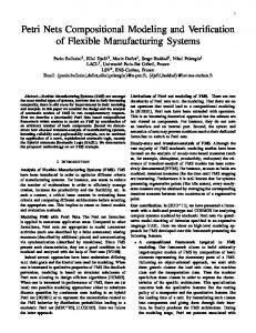
Fig. 7—Methane composition in the gas phase for various grid refinements by the MFE-DG and MFE-FD methods: Example 1, PV injection=0.41, dimensions in meter. September 2006 SPE Journal

345

Fig. 8—Methane composition in the gas phase for various grid refinements by the MFE-DG and MFE-FD methods: Example 1, PV injection=0.82, dimensions in meter.

sults from the MFE-DG method to those from the MFE-FD method. In the MFE-FD method, the shape functions for the DG method are assumed to be constant. In this case, the DG method is reduced to the first-order upstream FD method. In all our comparisons, we use the single-point upstream weighting scheme with the first-order FD method. Example 1. In this example, we consider a 2D horizontal domain with four connected fractures. The fracture configuration is shown in Fig. 4. The domain area is 100×100 m2. Methane is injected at one corner to displace propane, which saturates the domain, to the opposite producing corner (see Table 1). At the production well, the pressure is kept constant and equal to the initial pressure. In Figs. 7 and 8, the composition profile of C1 calculated by the MFE-FD and MFE-DG codes is shown at 41 and 82% PV injection. Different griddings (40×40, 60×60, and 100×100) are used to examine the solution convergence. The results by the MFE-FD method have a pronounced numerical dispersion compared to the MFE-DG solution. The MFE-DG method for a 40×40 gridding introduces less numerical dispersion than the MFE-FD on a 100×100 grid (see Figs. 7 and 8). There is significant merit in using the higher-order approximation in the DG method.

We use a sugar-cube configuration for the fractures (see Fig. 5). The relevant data for fluid, fracture, and rock properties are given in Table 2. The composition profiles of methane and propane in the oil and gas phases at three different positions (at Points A, B, and C, see Fig. 5) in the domain are depicted vs. the injected PV in Figs. 9 and 10. The reference solution is obtained by the MFEDG method on a 100×100 grid. The MFE-FD solution shows significant numerical dispersion compared to the MFE-DG solution. Example 3. This example is chosen to show the effect of fractures on the compositional flow performance by injecting gas in the fractured and unfractured media. The fluid system in Example 1 is used in this example. The matrix and fracture permeabilities are 10

Example 2. We consider the displacement of a binary liquid mixture of C2/C3 by a gas mixture of C1/C3. The gas (90% of C1 and 10% of C3) is injected at one corner of the 2D fractured domain. 346

September 2006 SPE Journal

Fig. 9—Methane composition in the gas and liquid phases at different points vs. the injected PV by the MFE-DG and MFE-FD methods: Example 2 (grid 30×30).

md and 106 md, respectively. The fracture aperture is 1 mm. The relevant data for fluid, rock, and fracture properties are presented in Table 1. The fracture configuration can be seen in Fig. 6. The compositional contours of methane in the fractured and unfractured domains are depicted in Fig. 11 at 0.13, 0.31, and 1.2 PV. In Fig. 12, we show the methane composition at the production well vs. the injected PV. Summary and Conclusions In Hoteit and Firoozabadi (2006), we demonstrated the superiority of the MFE-DG method over the single-point upstream weighting FD method in compositional modeling. In this work, we have extended the MFE-DG method to the compositional modelSeptember 2006 SPE Journal

ing in fractured media. The following are introduced in the extension: 1. Fluid flux between the matrix and the fracture is based on the assumption that the pressure and the concentration unknowns in a fracture element are equal to those in the adjacent cells that have the fracture element in common. This technique allows eliminating the calculation of the flux between the fracture and the matrix. 2. The MFE method is used to approximate the pressure and the total flow velocity along the fractures. The degrees of freedom of this approximation are the pressure average over the fracture element, the pressure traces, and the volumetric fluxes across the element extremities. The MFE method allows the representation of the fracture entity by the cell edges. 347

Fig. 10—Methane composition in the gas and liquid phases at different points vs. the injected PV by the MFE-DG and MFE-FD methods: Example 2 (grid 60×60).

We also presented a new method to calculate the fracture/ fracture flux in two-phase flow. Generally, the cell-based finiteelement methods face difficulty to approximate flow in multiintersecting fractures. As mentioned previously, the MFE approximation in the fractures provides, in addition to the pressure element averages, the pressure traces and the fluxes across the elements. Consequently, the MFE approximation does not need a special treatment even with gravity. One simply writes the material balance equations at the intersection node. Our method allows natural evaluation of the upstream function values. Nomenclature c ⳱ overall molar density, mole/m3 c␣ ⳱ molar density of the ␣ phase, mole/m3 e ⳱ node of fracture elements 348

E f fgi foi g kr␣ K K␣ nc Ne NE Nf NK p

⳱ ⳱ ⳱ ⳱ ⳱ ⳱ ⳱ ⳱ ⳱ ⳱ ⳱ ⳱ ⳱ ⳱

mesh edge 1D fracture element fugacity of component i in gas phase fugacity of component i in oil phase acceleration of gravity, m/s2 relative permeability mesh cell effective mobility, m.s/kg number of components number of edges of a cell number of edges number of intersecting fracture elements number of cells in a mesh pressure, Pa September 2006 SPE Journal

Fig. 11—Methane composition in the gas phase in homogeneous and fractured domains for various PV injection by the MFE-DG method: Example 3, dimensions in meter.

qf,e qK,E t T tp Ui wf,e wK,E xi␣ zi ␽

⳱ ⳱ ⳱ ⳱ ⳱ ⳱ ⳱ ⳱ ⳱ ⳱ ⳱

flux across edge e in f flux across edge E in K time, s temperature, K pressure trace, Pa molar flux of component i RT0 basis function in the line element RT0 basis function in the surface element mole fraction of component i in phase ␣ overall mole fraction of component i total velocity, m/s

September 2006 SPE Journal

␽␣ ␮ ␯i ␰ ␳␣ ␾

⳱ ⳱ ⳱ ⳱ ⳱ ⳱

velocity of phase ␣, m/s viscosity, kg/m/s total partial molar volume of i total fluid compressibility mass density of phase ␣, kg/m3 porosity, %

Acknowledgments This work was supported by the member companies of the Reservoir Engineering Research Inst. (RERI). This support is greatly appreciated. 349

Fig. 12—Methane composition at the production well vs. the PV injection for homogeneous and fractured domains by the MFEDG method: Example 3.

References Ács, G., Doleschall, S., and Farkas, É. 1985. General Purpose Compositional Model. SPEJ 25 (4): 543–553. SPE-10515-PA. Arbogast, T., Douglas, J., and Hornung, U. 1990. Derivation of the double porosity model of single phase via homogenization theory. SIAM J. Math. Anal. 21 (4): 823–836. Baca, R., Arnett, R., and Langford, D. 1984. Modeling fluid flow in fractured porous rock masses by finite element techniques. Int. J. Num. Meth. Fluids 4: 337–348. Bastian, P., Chen, Z., Ewing, R.E., Helmig, R., Jakobs, H., and Reichenberger, V. 2000. Numerical solution of multiphase flow in fractured porous media. Numerical Treatment of Multiphase Flows in Porous Media. Z. Chen, R.E. Ewing, and Z.C. Shi (eds.). Berlin: SpringerVerlag. Bourgeat, A. 1984. Homogenized behavior of diphasic flow in naturally fissured reservoir with uniform fractures. Comp. Methods in Applied Mechanics and Engineering 47: 205–217. Brezzi, F. and Fortin, M. 1991. Mixed and Hybrid Finite Element Method. New York: Springer-Verlag. Chavent, G. and Cockburn, B. 1989. The local projection P 0 P 1 discontinuous Galerkin finite element method for scalar conservation laws. M2AN 23 (4): 565–592. Chavent, G. and Jaffré, J. 1986. Mathematical Models and Finite Elements for Reservoir Simulation, Studies in Mathematics and its applications. North Holland, Amsterdam: Elsevier Science Publishing Co. Chavent, G. and Roberts, J-E. 1991. A unified physical presentation of mixed, mixed-hybrid finite element method and standard finite difference approximations for the determination of velocities in water flow problems. Adv. Water Resour. 14 (6): 329–348. Chen, Z. and Ewing, R. 1997a. Comparison of various formulations of the three-phase flow in porous media. J. Comp. Phys. 132: 362–373. Chen, Z. and Ewing, R. 1997b. From single-phase to compositional flow: applicability of mixed finite elements. Transport in Porous Media 27: 225–242. Cockburn, B. and Shu, C. 1989. TVB Runge Kutta local projection discontinuous Galerkin finite element method for conservative laws II: General frame-work. Math. Comp. 52: 411–435. Cockburn, B. and Shu, C. 1998. The Runge-Kutta Discontinuous Galerkin Method for Conservative Laws V: Multidimentional Systems. J. Comput. Phys. 141: 199–224. Cockburn, B. and Shu, C. 2001. Runge-Kutta discontinuous Galerkin method for convection-dominated problems. J. Scientific Computing 16 (3): 173–261. Durlofsky, L.J. and Chien, M.C.H. 1993. Development of a Mixed FiniteElement-Based Compositional Reservoir Simulator. Paper SPE 25253 presented at the SPE Symposium on Reservoir Simulation, New Orleans, 28 February–3 March. 350

Ewing, R.E. and Heinemann, R.F. 1983. Incorporation of Mixed Finite Element Methods in Compositional Simulation for Reduction of Numerical Dispersion. Paper SPE 12267 presented at the SPE Reservoir Simulation Symposium, San Francisco, 15–18 November. Ghorayeb, K. and Firoozabadi, A. 2000. Numerical Study of Natural Convection and Diffusion in Fractured Porous Media. SPEJ 5 (1): 12–20. SPE-51347-PA. Granet, S., Fabrie, P., Lemmonier, P., and Quitard, M. 1998. A single phase simulation of fractured reservoir using a discrete representation of fractures. Paper presented at the European Conference on the Mathematics of Oil Recovery, Peebles, Scotland, U.K., 8–11 September. Granet, S., Fabrie, P., Lemonnier, P., and Quitard, M. 2001. A two-phase flow simulation of a fractured reservoir using a new fissure element method. J. Petroleum Science and Engineering 32 (18): 35–52. Hoteit, H. and Firoozabadi, A. 2005. Multicomponent fluid flow by discontinuous Galerkin and mixed methods in unfractured and fractured media. Water Resour. Res. 41 (11): 1–15. W11412, doi:10.1029/ 2005WR004339. Hoteit, H. and Firoozabadi, A. 2006. Compositional Modeling by the Combined Discontinuous Galerkin and Mixed Methods. SPEJ 11 (1): 19– 34. SPE-90276-PA. Hoteit, H., Ackerer, P., Mosé, R., Erhel, J., and Philippe, B. 2004. New Two-Dimensional Slope Limiters for Discontinuous Galerkin Methods on Arbitrary Meshes. Int. J. Numer. Meth. Eng. 61 (14): 2566–2593. Karimi-Fard, M. and Firoozabadi, A. 2003. Numerical Simulation of Water Injection in Fractured Media Using the Discrete Fractured Model and the Galerkin Method. SPEREE 6 (2): 117–126. SPE-71615-PA. Karimi-Fard, M., Durlofsky, L.J., and Aziz, K. 2004. An Efficient Discrete-Fracture Model Applicable for General-Purpose Reservoir Simulators. SPEJ 9 (2): 227–236. SPE-79699-PA. Kazemi, H. 1969. Pressure Transient Analysis of Naturally Fractured Reservoirs With Uniform Fracture Distribution. SPEJ 9 (12): 451–462; Trans., AIME, 246. SPE-2156A-PA. Kim, J.G. and Deo, M.D. 1999. Comparison of the performance of a discrete fracture multiphase model with those using conventional methods. Paper SPE 51928 presented at the SPE Reservoir Simulation Symposium, Houston, 14–17 February. Kim, J.G. and Deo, M.D. 2000. Finite element discrete fracture model for multiphase flow in porous media, AIChE J. 46 (6): 1120–1130. Mallison, B., Gerritsen, M., Jessen, K., and Orr F.M. 2005. High-order Upwind Schemes for Two-Phase, Multicomponent Flow. SPEJ 10 (3): 291–311. SPE-79691-PA. Monteagudo, J. and Firoozabadi, A. 2004. Control-volume method for numerical simulation of two-phase immiscible flow in 2D and 3D discrete-fracture media. Water Resour. Res. 7: 1–20. doi:10.1029/ 2003WR002996. Noorishad, J. and Mehran, M. 1982. An upstream finite element method for the solution of transient transport equation in fractured porous media. Water Resour. Res. 18 (3): 588–596. Peddibhotla, S., Datta-Gupta, A., and Xue, G. 1997. Multiphase Streamline Modeling in Three Dimensions: Further Generalizations and a Field Application. Paper SPE 38003 presented at the SPE Reservoir Simulation Symposium, Dallas, 8–11 June. Putti, M., Yeh, W., and Mulder, W. 1990. A triangular finite volume approach with high-resolution upwind terms for the solution of groundwater transport equations. Water Resour. Res. 26 (12): 2865–2880. Raviart, P. and Thomas, J. 1977. A mixed hybrid finite element method for the second order elliptic problem. Lectures Notes in Mathematics 606. New York: Springer-Verlag, 292–315. Rivière, B., Wheeler, M.F., and Banas, K. 2000. Part II. Discontinuous Galerkin Method Applied to Single Phase Flow in Porous Media. Computational Geosciences (2000) 4 (4): 337–341. Rubin, B. and Blunt, M.J. 1991. Higher-Order Implicit Flux-Limiting Schemes for Black Oil Simulation. Paper SPE 21222 presented at the SPE Symposium on Reservoir Simulation, Anaheim, California, 17–20 February. Tan, C. and Firoozabadi, A. 1995. Theoretical analysis of miscible displacement in fractured porous media: I. Theory. J. Can. Petrol. Technol. 34 (2): 17–27. Thomas, L.K., Dixon, T.N., and Pierson, R.G. 1983. Fractured Reservoir Simulation. SPEJ 23 (1): 42–54. SPE-9305-PA. September 2006 SPE Journal

Warren, J.E. and Root, P.J. 1963. The Behavior of Naturally Fractured Reservoirs. SPEJ 3 (11): 245–255; Trans., AIME, 228. Watts, J. 1986. A Compositional Formulation to the Pressure and Saturation Equations. SPERE 1 (3): 243–252; Trans., AIME, 281. SPE12244-PA.

兰w

−1 K,EKK wK,E⬘

BK = 关共BK兲E,E⬘ 兴E,E⬘∈⭸K; 共BK兲E,E⬘ =

K

兰w

B˜ K = 关共B˜ K兲E,E⬘ 兴E,E⬘∈⭸K; 共B˜ K兲E,E⬘ =

K,EwK,E⬘

K

Appendix In this appendix, we provide details of the approximation of the pressure and velocity field by the MFE method. The MFE method, which is based on the lowest-order Raviart-Thomas space, approximates separately the total velocity equation (Eq. 6) and the pressure equation (Eq. 14). Approximation of the Total Velocity Equation. From the Raviart-Thomas approximation space, the vectors ␽ and g over each element K can be expressed in terms of the lowest-order RaviartThomas basis function wK,E and the fluxes across the element boundaries; that is,

兺q

␽=

K,EwK,E

where qK,E =

兺q

g=

and

E∈⭸K

g K,EwK,E,

. . . . . . . . . . . . (A-1)

E∈⭸K

兰 ␽.n

兰 g.n

g qK,E =

and

K,E

K,E = g|E| cos关Ang共g,nK,E兲兴.

E

Multiplying Eq. A-2 by the basis function wK,E and integrating by parts yields K,EK

兰

J = − wK,E共ⵜp − ␳g兲

K

K

兰

K,E

−

E⬘∈⭸K

共␤K兲E,E⬘ = 共BK−1兲E,E⬘,

qf,e = ␪f,epf −

E = E⬘

0

if

E ⫽ E⬘.

. . . . . . . . . . . . . . . . . . . . . . . (A-5)

K

兰p − |E | 兰p + 兰␳w 1

K

K,Eg

E

E ∈ ⭸K.

K

. . . . . . . . . . . . . . . . . . . . . . . . (A-6)

Let pK and tpK,E denote the cell average pressure on K and the edge average pressure on E, respectively (that is, the first and the second terms on the right side of Eq. A-6). Replace Eq. A-1 in Eq. A-6 to get

兺 q 兰w

−1 K,EKK wK,E⬘

K,E⬘

E⬘∈K

K

K

f

f

⭸f

dpK = dt

兺 ␳ q 兰w

E⬘∈K

K,EwK,E⬘

BKQK = pKe − TpK − ␳KB˜ KQKg , . . . . . . . . . . . . . . . . . . . . . . . . (A-8)

September 2006 SPE Journal

兺 v 冉兺 m

i,K,eqK,e

i,f

− s˜i,K,e , . . . . . . . . . . . . . (A-13)

e∈⭸f

where ␵K,f = 共␾K␰K|K | + | f | ␾f ␰f兲, s˜i,K,E =

兰 共s

and s˜i,f,e =

i,K.nK,E 兲,

兰 共s .n i,f

f,e 兲.

E

Eq. A-13 can be written in terms of the pressure and the traces of the pressure unknowns by placing Eqs. A-9 and A-10 into Eq. A-13; that is,

␵K,f

⭸pK = ␣˜ KpK − ␤˜ K,EtpK,E − ␤˜ f,etpf,e + ␥˜ K, . . . . . (A-14) ⭸t E∈⭸K e∈⭸f

兺

兺

where

兺 v˜

nc

K,E␪K,E;

v˜ K,E =

␤˜ K,E =

兺 v˜

E⬘∈⭸K

兺 共v

i,Kmi,K,E 兲

i=1

K,E⬘共␤K 兲E,E⬘; ˜␤f,e = ␧

兺

v˜ f,e⬘共␤f兲e,e⬘

e⬘∈⭸f

K

Eq. A-7 can be written in matrix form

where

E∈⭸K

E∈⭸K

E ∈ ⭸K. . . . . . . . . (A-7)

冊 冊

− s˜i,K,E

i,K,EqK,E

i,K

i=1 nc

i=1

␣˜ K =

= pK − tpK,E⬘

g K K,E⬘

兺v 冉兺 m nc

+␧

K

+

e ∈ ⭸f. . . . . . . . . . . . (A-10)

⭸K

E

Using Eqs. A-4 and A-5, the integral terms in the right side of Eq. A-3 are simplified to 1 |K |

− ␥f,e,

兰共␽ .n 兲, . . . . . . . . . . . . . . . . . . . . . . . . . . . . . . (A-11)

=

E∈⭸f

␵K,f

if

=

f e,e⬘tpf,e⬘

Approximation of the Pressure Equation. The fluxes across the boundaries of a matrix element K and the ends of a fracture element f are defined, respectively, as

E ∈ ⭸K. . . . . . . . . . . . . . . . . . . . . (A-3)

K,Eg

1 Ⲑ |E |

−1 K,EK ␽

兺 共␤ 兲

e⬘∈⭸f

f,E

K,E.nK,E

1 , . . . . . . . . . . . . . . . . . . . . . . . . . . . . . . . . . . . . . . . (A-4) ⵜ.wE = |K |

兰w

−1 ˜ g K BK 兲E,E⬘qK,E⬘.

In a similar way, the flux at the 1D fracture ends is written as

The Raviart-Thomas basis function wK,E satisfies the following properties:

再

兺 共B

and ␥K,E = −␳K

兺 q = 兰共␽ .n 兲. . . . . . . . . . . . . . . . . . . . . . . . . . . . . . . . . (A-12)

兰pw

K

wE.nE⬘ =

−1 K 兲E,E⬘,

Replacing Eqs. A-11 and A-12 in Eq. 15 yields

兰␳w

+

E ∈ ⭸K, . . . . . (A-9)

兺 共B

␪K,E =

⭸K

K

tpK,E⬘ − ␥K,E ,

where,

E∈⭸K

K

兰pⵜ.w

K E,E⬘

E⬘∈⭸K

K,E

K,Eg

K

兺 共␤ 兲

qK,E = ␪K,EpK −

兺q

兰␳w

= − wK,Eⵜp + =

By inverting BK in Eq. A-8, the flux qK,E through each edge E is expressed as a function of the cell pressure average pK and the edge pressure averages tpK,E , or

E⬘∈⭸K

K−1␽ = −共ⵜp − ␳g兲. . . . . . . . . . . . . . . . . . . . . . . . . . . . . . . . . (A-2)

兰w

TpK = 关tpK,E兴E∈⭸K; e = 关1兴E∈⭸K.

E

By inverting the mobility tensor K, Eq. 6 becomes

−1

g QK = 关qK,E兴E∈⭸K; QKg = 关qK,E 兴E∈⭸K;

␥˜ K =

兺 v˜

E∈⭸K

nc

K,E␥K,E

+

兺v

˜i,K,E i,Ks

i=1

+␧

兺 v˜ e∈⭸f

nc

f,e␥f,e

+␧

兺 v s˜

i,f i,f,e.

i=1

. . . . . . . . . . . . . . . . . . . . . . . .(A-15) 351

Hussein Hoteit is a scientist at the RERI in Palo Alto, California. His research interests include numerical modeling of multiphase miscible and immiscible flow in homogeneous and fractured media. He holds MS and PhD degrees in applied mathematics from U. Rennes 1, France. Abbas Firoozabadi is a senior scientist and director at RERI. He also teaches at Yale U. and at Imperial College, London. e-mail: [email protected]. His main research activities center on thermo-

352

dynamics of hydrocarbon reservoirs and production and on multiphase/multicomponent flow in fractured petroleum reservoirs. Firoozabadi holds a BS degree from Abadan Inst. of Technology, Abadan, Iran, and MS and PhD degrees from the Illinois Inst. of Technology, Chicago, all in gas engineering. Firoozabadi is the recipient of both the 2002 SPE Anthony Lucas Gold Medal and the 2004 SPE John Franklin Carll Award.

September 2006 SPE Journal