Sep 17, 2007 - This note applies conditional density estimation as a visual method to present results. The proposed method is illustrated by application to a ...
Conditional density estimation: an application to the Ecuadorian manufacturing sector Kim Huynh
David Jacho-Chavez
Indiana University
Indiana University
Abstract This note applies conditional density estimation as a visual method to present results. The proposed method is illustrated by application to a firm-level manufacturing data set from Ecuador in 2002.
We acknowledge the usage of the R package -hdrcde- by Hyndman and Einbeck (2006). We also acknowledge the usage of the Libra High Performance Cluster at Indiana University where the computations were performed. All remaining errors are our own. Citation: Huynh, Kim and David Jacho-Chavez, (2007) "Conditional density estimation: an application to the Ecuadorian manufacturing sector." Economics Bulletin, Vol. 3, No. 62 pp. 1-6 Submitted: September 17, 2007. Accepted: November 14, 2007. URL: http://economicsbulletin.vanderbilt.edu/2007/volume3/EB-07C10008A.pdf
1
Introduction
This note documents some empirical facts for the manufacturing sector in Ecuador. Understanding the manufacturing sector in less developed countries (LDCs) is of first-order importance for economists and policymakers. Tybout (2000) provides an overview of the literature on manufacturing firms in developing countries. Our contribution is to apply conditional density estimation to a recently released firm-level manufacturing database from Ecuador. This approach is a nonparametric approach to empirically describing the data without making any structural assumptions. Since it is descriptive in nature, potential problems with causality, endogeneity, functional forms, and sample selection do not need to be considered. We compare and contrast standard descriptive statistics with conditional density estimation. We illustrate the utility of conditional density estimation as a tool to explore relationships between a response and explanatory variables. The rest of the note is as follows: Section 2 discusses the conditional density estimation approach. Section 3 describes the data and discusses the findings, while Section 4 concludes.
2
Kernel Estimation of Conditional Densities
Let Y and X be two scalar random values defined on ℜ, with joint probability density function fY,X (·, ·), and X having a marginal density fX (·). Then, the conditional probability density function of Y given X = x is fY,X (y, x) f Y |X ( y| x) = . (2.1) fX (x) Given a random sample {Yi , Xi }N i=1 , consistent kernel-based estimators of (2.1) can be written in the form N X fbY |X ( y| x) = wi (x) Khy (y − Yi ) , (2.2) i=1
where wi (·) is a weighting function, and Kh (u) = h−1 K (u/h), where the kernel function, K (·), is a real, integrable, non-negative, even function on ℜ such that Z Z Z K (u) du = 1, uK (u) du = 0, u2 K (u) du < +∞, ℜ
ℜ
ℜ
and h is a bandwidth parameter. Different choices of weighting functions, wi (·), gives consistent estimators with different bias and variance properties. See Hyndman et al. (1996), Fan et al. (1996), De Gooijer and Zerom (2003), and Hansen (2004) for example. In this letter, the empirical application is based on the local constant weights wi (x) = Khx (x − Xi ) /
N X
Khx (x − Xj ) ,
(2.3)
j=1
with the gaussian kernel. This estimator corresponds to estimating (2.1) by the ratio of two kernel density estimators, i.e. fbY,X (y, x) fbY |X ( y| x) = (2.4) fbX (x) 1
(see Rosenblatt (1969)). Hyndman et al. (1996) shows that in the limit, if hx → 0, hy → 0, and N hx hy → +∞, as N → ∞, fbY |X ( y| x) is a consistent estimator for f Y |X ( y| x).
3
Data and Empirical Application
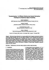
The data set is drawn from a cross section of firms in two specific manufacturing industries in Ecuador. The sample consists of 736 firms in the Food and Beverages industry, and 386 firms in the Petroleum, Chemical and Plastics industry, taken from the 2002 Manufacturing and Mining Survey (Encuesta de Manufactura y Miner´ıa) prepared by the Ecuadorian National Institute of Statistics and Census (Instituto Nacional de Estad´ıstica y Censos - INEC). For each firm we observe the net value of real fixed assets K, the number of employees L, and the value-added real output Y . K and Y are measured in thousands of dollars. Specifically, we describe the following relationships with a table of conditional moments and conditional densities: 1. Capital-labour ratio (K/L) and the output of the firm (Y ), 2. Firm size (L) and the output of the firm (Y ), 3. Labour productivity (Y /L) and the output of the firm (Y ). Table 1 computes some standard conditional moments for both industries at different quantiles of Y . The tables are informative as they show the central and dispersion characteristics of the data across different output levels. Alternatively, the conditional density plots summarizes the data by showing the entire conditional distribution. Figures 1 shows the results. These ‘stacked conditional density’ plots1 are bias-corrected and show scaled conditional densities at different levels of the conditioning variables. We implement kernel-based estimate (2.2) with local constant weights (2.3) using a gaussian kernel, and bandwidths chosen using the normal reference rules of Bashtannyk and Hyndman (2001). From the conditional densities the Food and Beverage industry has a capital-to-labour ratio that is disperse and skewed towards labour intensity for lower output levels. As output increases the distribution of capital-to-labour ratio increases and the distribution is less-dispersed. For the Petroleum, Chemical, and Plastics industry a similar story appears except that at lower output levels the distribution is somewhat bimodial and is skewed towards capital intensity. The results follow intuition that the Chemicals & Plastics industry is skewed towards capital-intensity than the Food & Beverage industry. In terms of firm size (in terms of employment) and output levels the Food Beverage and Petroleum, Chemical, and Plastics industry shows a positive relationship, larger output levels are associated with larger size of firm. However, the dispersion is higher with the Petroleum, Chemical, and Plastics industry. For labour productivity the pictures indicate a similar story: the dispersion is higher with the Petroleum, Chemical, and Plastics industry. This result confirms the findings of Tybout (2000) 1
They were created using the library hdrcde by Hyndman and Einbeck (2006) in the statistical environment R.
2
that found that the cross-sectional variation in firm productivity is high in LDCs. However, we are able to see that the dispersion is higher in the Petroleum, Chemical, and Plastics industry. Finally, all the plots show a clear pattern of conditional mean dependence. This is important for modeling purposes, as it can potentially justify many popular parametric functional forms for the relationship between output of the firm and its inputs. For example, the labour productivity and output conditional density illustrates a quadratic relationship. The conditional mean of labour productivity increases for low-to-medium ranges of output then slightly decreases at higher ranges of output. The other relationships, such as the capital-labour ratio for the Petroleum, Chemical, and Plastics, illustrates a clear linear relationship in the conditional mean.
4
Conclusion
In this note, we have proposed the usage of a visual device, known as nonparametric kernel density estimator, to explore relationships among economic variables, without the need of a structural model. Applying these tools allows us to summarize the results in concisely in a three-dimensional plots. The three-dimensional plots provide much more information than using tables as it provides information on the entire distribution instead of snapshot. Future extensions will include a methodology to summarize multivariate conditional estimators with ordered or discrete data (e.g. level of export/import intensity).
References Bashtannyk, David M., and Rob J. Hyndman, 2001, Bandwidth selection for kernel conditional density estimation, Computational Statistics & Data Analysis 36, 279–298. De Gooijer, Jan G., and Dawit Zerom, 2003, On conditional density estimation, Statistica Neerlandica 57(2), 159–176. Fan, Jianquing, Qiwei Yao, and Howell Tong, 1996, Estimation of conditional densities and sensitivity measures in nonlinear dynamical systems, Biometrika 83(1), 189–206. Hansen, Bruce E., 2004, Nonparametric conditional density estimation, Unpublished Manuscript. Hyndman, Rob, and Jochen Einbeck, 2006, hdrcde: Highest density regions and conditional density estimation. R package version 2.02. Hyndman, Rob J., David M. Bashtannyk, and Gary K. Grunwald, 1996, Estimating and visualizing conditional densities, Journal of Computational and Graphical Statistics 5(4), 315–336. Rosenblatt, M., 1969, Conditional probability density and regression estimators, in: P. R. Krishnaiah, ed., Multivariate Analysis II(Academic Press, New York) 25–31. Tybout, James R., 2000, Manufacturing firms in developing countries: How well do they do, and why?, Journal of Economic Literature 38(1), 11–44. 3
Table 1: Conditional Moments
Output 20% - 30% 45% - 55% 70% - 80%
Capital-Labour Ratio Food & Beverages Petroleum, Chemical & Plastics mean median s.d. mean median s.d. 5.366 12.013 21.956
2.792 6.879 12.010
Output
mean
Firm Size (Employment) median s.d. mean median
20% - 30% 45% - 55% 70% - 80%
2125.676 3785.135 8648.648
2000 3600 7745
Output
mean
median
20% - 30% 45% - 55% 70% - 80%
2.804 5.099 8.636
2.794 4.399 6.966
a
6.859 13.868 22.485
823.966 1961.316 4721.626
7.721 19.080 24.275
2253.846 4139.473 6469.230
6.114 11.019 18.011
1800 3850 5000
Labour Productivity s.d. mean median 0.894 2.527 5.552
4.384 6.853 13.071
4.534 6.011 11.717
6.023 23.145 22.354
s.d. 1155.956 2398.709 4754.399
s.d. 1.682 3.733 6.669
For each industry, the descriptive statistics were constructed as follows: We calculate the 20, 30, 45, 55, 70 and 80% empirical quantile of observed output. Then, firms are classified in three groups based on whether their output are between the 20% - 30%, 45% - 55%, and 70% - 80% empirical quantiles. The above descriptive statistics are calculated within each group.
4
Capital−Labour Ratio & Output Food & Beverages
Petroleum, Chemical & Plastics
14
14
12
12
10
8 4
2 ln(K/L)
6
4
2 ln(K/L)
6
0
−2
−4
ln(Y)
6
ln(Y)
10
8 0 −2
Employment & Output
14
14
12
12
10
8
12
12 10 ln(L)
11
10
6
8
9
ln(L)
6
ln(Y)
ln(Y)
10
8 8
7
6
Labour Productivity & Output
14
14
4
10
8 2 ln(Y/L)
0
−2
4
6
3
2 1 ln(Y/L)
0
Figure 1: Estimated Conditional Densities
5
8 −1
ln(Y)
6
ln(Y)
12 10
12