Nov 6, 2013 - parameter estimation also has been implemented to online estimate model ... Nachbarzimmern Steffen und Johannes für die vielen schönen Stunden, nicht nur während ...... Cambridge University Press, 2 edition, April 2006.
Control System Theoretic Approach to Model Based Navigation Vom Fachbereich Maschinenbau an der Technischen Universit¨at Darmstadt zur Erlangung der W¨ urde eines Doktor-Ingenieurs (Dr.-Ing.) genehmigte Dissertation
von
Dipl.-Ing. Alexander Sendobry
geboren am 1. Juli 1982 in Groß-Gerau
1. Gutachten 2. Gutachten
Prof. Dr.-Ing. Uwe Klingauf Prof. Dr.-Ing. habil. Gert Franz Trommer
Tag der Einreichung Tag der m¨ undlichen Pr¨ ufung
11. Juni 2013 6. November 2013
D17
Meinen Eltern
Abstract This thesis gives an overview and classification of current conventional and model based navigation algorithms found in the literature. Model based in that context means, that a mathematical/physical system model of the moving vehicle is integrated into the Kalman Filter, which normally performs the state estimation task. In contrast to conventional navigation algorithms, which rely solely on inertial measurements for the prediction of states, model based approaches have the great advantage, that a prediction is possible even when no measurements are available. The architecture of the new Full State Vehicle Dynamics (FSVD) algorithm is based on the principals of state estimation using a Luenberger observer or Kalman Filter, which in general runs parallel to the technical system, whose states need to be estimated. Current conventional and model based navigation algorithms are described and compared mathematically. In a next step a comprehensive evaluation of all algorithms took place. Therefore two different examples are given. On the one hand an autonomous flying vehicle which is evaluated in simulations and on the other hand a real navigation test vehicle, which is a van with numerous sensors on board. Low cost sensors which aid the model based navigation solution and high-end sensors which serve as reference system for validation. For both systems the mathematical system description is given and results are presented. In the ideal case, where reference model and filter implementation have the same parametrization, no differences between all model based algorithms can be found. But as soon as different parameters in reference and filter model occur, the FSVD algorithm shows a better performance than the other model based algorithms. Estimated quantities of the FSVD also have smoother characteristics compared to conventional and other model based approaches. For completeness, and to show the ease of state vector augmentation, the possibility of parameter estimation also has been implemented to online estimate model parameters.
I
Zusammenfassung Die Arbeit beschreibt aktuell genutzte konventionelle und modellbasierte Navigationsalgorithmen in einem systemtheoretischen Kontext. Dabei bedeutet modellbasiert, dass eine mathematische/ physikalische Beschreibung des sich bewegenden Objekts existiert, die innerhalb eines Kalmanfilters die Zustandssch¨atzung u ¨bernimmt. Im Gegensatz zu konventionellen Navigationsalgorithmen, die aufgrund von inertial gemessenen Gr¨oßen eine Zustandsberechnung durchf¨ uhren, kann ein modellbasierter Algorithmus auch eine L¨osung liefern, wenn gerade keine Messwerte vorliegen. Aufbauend auf den Grundgedanken des Luenberger Beobachters und Kalmanfilters wird eine Systemarchitektur vorgestellt, die komplett parallel zu dem eigentlichen technischen System l¨auft und durch beliebige Messungen gest¨ utzt werden kann - der Full State Vehicle Dynamics (FSVD) Algorithmus. Der Ausdruck leitet sich aus dem Umstand ab, dass der komplette Zustandsvektor des Systems berechnet wird, basierend auf Kenntnis der Systemdynamik. Zum besseren Verst¨andnis werden alle verglichenen Algorithmen in einheitlicher mathematischer Notation vorgestellt. Nach der mathematischen Beschreibung erfolgt eine umfassende Untersuchung der verschiedenen Algorithmen an zwei Beispielen. Zum einen wurde ein Simulationsmodell eines Quadrokopters aufgebaut, an dem die Vor- und Nachteile der Ans¨atze aufgezeigt werden. Zum anderen wurde der FSVD Algorithmus benutzt, um mit mathematischem Systemwissen und g¨ unstigen Sensoren die Bewegung eines realen Forschungsfahrzeugs zu sch¨atzen. Zus¨atzlich war dieses Fahrzeug mit einem pr¨azisen Referenzmesssystem ausgestattet, um eine Aussage u ute des FSVD treffen zu k¨onnen. ¨ber die G¨ Es konnte gezeigt werden, dass alle Algorithmen sehr ¨ahnliche Ergebnisse liefern, solange das reale System und das interne Modell identisch sind - die Mathematik hinter allen Ans¨atzen ist dieselbe. Sobald aber Parameterschwankungen auftreten sind die Sch¨atzergebnisse des FSVD denen der anderen Verfahren u ¨berlegen und deutlich glatter im Verlauf der Sch¨atzgr¨oßen. Eine Parametersch¨atzung ist mit dem FSVD ebenfalls einfacher m¨oglich, als mit den anderen vorgestellten Algorithmen.
II
Vorwort Die vorliegende Arbeit entstand w¨ahrend meiner f¨ unfj¨ahrigen T¨atigkeit als wissenschaftlicher Mitarbeiter am Institut f¨ ur Flugsysteme und Regelungstechnik (FSR) der TU Darmstadt unter Leitung von Herrn Prof. Dr.-Ing. Uwe Klingauf. Ihm, als meinem Doktorvater, geb¨ uhrt mein besonderer Dank sowohl f¨ ur die vielen Freiheiten, die er mir bei der Wahl und Bearbeitung des Themas lies, als auch f¨ ur das entgegengebrachte Vertrauen. Prof. Dr.-Ing. habil. Gert Franz Trommer gilt ebenfalls mein besonderer Dank f¨ ur die ¨ Ubernahme des Koreferats und das damit bekundete Interesse an meiner Arbeit. Bei allen Kollegen des Instituts m¨ochte ich mich f¨ ur die angenehme Atmosph¨are bedanken, die mir f¨ unf wirklich sch¨one Jahre bescherte. Insbesondere gilt mein Dank meinem langj¨ahrigen Zimmergenossen Martin und seinem Vorg¨anger Frank sowie den Jungs“ aus den ” Nachbarzimmern Steffen und Johannes f¨ ur die vielen sch¨onen Stunden, nicht nur w¨ahrend der Arbeitszeit. In euch habe ich richtig gute Freunde gefunden. Danken m¨ochte ich außerdem meinen studentischen Arbeitern, die durch ihre Arbeiten eine wertvolle Unterst¨ utzung f¨ ur mich waren. Des weiteren gilt mein Dank den beiden Dozenten, deren Vorlesung Grundlagen der Navigation ich betreuen durfte. Burkard und J¨ urgen, es hat mir immer sehr viel Freude bereitet, eure Vorlesung und vor allem auch die Pr¨ ufung zu betreuen. Ich konnte dabei sehr viel - nicht nur fachlich - lernen. Die Studienzeit mit meinen Kollegen Andreas, Carsten, Christian, Daniel, Fabian, Lisa, Michael, Paul, Thomas und Tobias hat uns zu dem gemacht hat, was wir sind. Ich freue mich immer wieder, dass sich unsere Wege gekreuzt haben. F¨ ur das Verst¨andnis und Vertrauen in mein Tun bedanke ich mich von ganzem Herzen bei meiner Frau Annette. Danke, dass es Dich gibt. Zuletzt m¨ochte ich nat¨ urlich meinen Eltern Beate und Eberhard und meinen Br¨ udern Sebastian und Florian danken. Eltern und Geschwister kann man sich nicht aussuchen, ich hatte ganz großes Gl¨ uck.
Darmstadt, im Juni 2013 Alexander Sendobry
III
Contents Abstract
I
Zusammenfassung
II
Symbols and Abbreviations Greek Symbols . . . . . . . Abbreviations . . . . . . . . Matrices . . . . . . . . . . . Roman Symbols . . . . . . . Subscripts and Superscripts Vectors . . . . . . . . . . . .
. . . . . .
. . . . . .
. . . . . .
. . . . . .
. . . . . .
. . . . . .
. . . . . .
. . . . . .
. . . . . .
. . . . . .
. . . . . .
. . . . . .
. . . . . .
. . . . . .
1 Motivation and Evolution of Navigation 1.1 Conventional Inertial Navigation Systems (INS) 1.2 Conventional Model-based Approaches . . . . . 1.2.1 External Vehicle Dynamics (ExVD) . . . 1.2.2 Embedded Vehicle Dynamics (EmVD) . 1.3 Model Based Navigation System (FSVD) . . . . 1.4 Structure of this work . . . . . . . . . . . . . .
. . . . . .
. . . . . .
. . . . . .
. . . . . .
. . . . . .
. . . . . .
. . . . . .
. . . . . .
2 Conventional and Model Based Navigation Algorithms 2.1 Full State Inertial Navigation System (FS-INS) . . . . 2.2 Error State Inertial Navigation System (ES-INS) . . . . 2.2.1 Implementation . . . . . . . . . . . . . . . . . . 2.3 External Vehicle Dynamics (ExVD) . . . . . . . . . . . 2.3.1 Implementation . . . . . . . . . . . . . . . . . . 2.4 Embedded Vehicle Dynamics (EmVD) . . . . . . . . . 2.4.1 Implementation . . . . . . . . . . . . . . . . . .
. . . . . .
. . . . . .
. . . . . . .
. . . . . .
. . . . . .
. . . . . . .
. . . . . .
. . . . . .
. . . . . . .
. . . . . .
. . . . . .
. . . . . . .
. . . . . .
. . . . . .
. . . . . . .
. . . . . .
. . . . . .
. . . . . . .
. . . . . .
. . . . . .
. . . . . . .
. . . . . .
. . . . . .
. . . . . . .
. . . . . .
. . . . . .
. . . . . . .
. . . . . .
. . . . . .
. . . . . . .
. . . . . .
. . . . . .
. . . . . . .
. . . . . .
. . . . . .
. . . . . . .
. . . . . .
VII VII VIII IX X XI XII
. . . . . .
1 4 5 5 6 7 10
. . . . . . .
11 11 12 13 14 16 18 19
3 New Model Based Navigation Algorithm with Observer Structure 23 3.1 Full State Vehicle Dynamics (FSVD) . . . . . . . . . . . . . . . . . . . . . . . 24 3.1.1 Implementation . . . . . . . . . . . . . . . . . . . . . . . . . . . . . . . 25 4 Modelling of two Example Systems 27 4.1 Rigid Body Motion . . . . . . . . . . . . . . . . . . . . . . . . . . . . . . . . . 28 4.1.1 Movement in a Local North pointing Reference System . . . . . . . . . 28
V
Contents 4.2
4.3 4.4
Quadrotor . . . . . . . . . . . . . . . . . . 4.2.1 Brushless DC Motor Controller . . 4.2.2 Brushless DC Motor . . . . . . . . 4.2.3 Propeller Thrust Generation . . . . 4.2.4 Forces and Moment Transformation 4.2.5 Cascaded Controller Structure . . . Navigation Test Vehicle . . . . . . . . . . Sensors . . . . . . . . . . . . . . . . . . . . 4.4.1 Deterministic Measurement Models 4.4.2 Stochastic Measurement Models . .
. . . . . . . . . .
. . . . . . . . . .
. . . . . . . . . .
. . . . . . . . . .
. . . . . . . . . .
5 Evaluation of Simulation and Measurement Results 5.1 Simulation Environment of the Quadrotor . . . . . 5.2 Qualitative Results and Characteristics . . . . . . . 5.3 Quantitative Results for the Quadrotor . . . . . . . 5.3.1 Systematic Errors . . . . . . . . . . . . . . . 5.3.2 Stochastic Errors . . . . . . . . . . . . . . . 5.3.3 Filter Convergence . . . . . . . . . . . . . . 5.3.4 Bias Estimation . . . . . . . . . . . . . . . . 5.3.5 Correlation Coefficient . . . . . . . . . . . . 5.3.6 Convergence with Parameter Variances . . . 5.3.7 Parameter Estimation Capability . . . . . . 5.4 Test Drive with the Navigation Test Vehicle . . . .
. . . . . . . . . .
. . . . . . . . . . .
. . . . . . . . . .
. . . . . . . . . . .
. . . . . . . . . .
. . . . . . . . . . .
. . . . . . . . . .
. . . . . . . . . . .
. . . . . . . . . .
. . . . . . . . . . .
. . . . . . . . . .
. . . . . . . . . . .
. . . . . . . . . .
. . . . . . . . . . .
. . . . . . . . . .
. . . . . . . . . . .
. . . . . . . . . .
. . . . . . . . . . .
. . . . . . . . . .
. . . . . . . . . . .
. . . . . . . . . .
. . . . . . . . . . .
. . . . . . . . . .
. . . . . . . . . . .
. . . . . . . . . .
. . . . . . . . . . .
. . . . . . . . . .
. . . . . . . . . . .
. . . . . . . . . .
29 32 34 35 37 37 38 40 40 46
. . . . . . . . . . .
51 51 54 55 56 57 67 72 77 81 86 89
6 Conclusion and Outlook 97 6.1 Outlook . . . . . . . . . . . . . . . . . . . . . . . . . . . . . . . . . . . . . . . 98 Bibliography Basics 1 Coordinate Systems . . . . . . . . . . . . . . . . . . . . . 1.1 Nomenclature of Variables . . . . . . . . . . . . . 1.2 Describing Rotation Sequences with Euler Angles 1.3 Describing Rotation Sequences with Quaternions 2 Kalman Filter . . . . . . . . . . . . . . . . . . . . . . . . 2.1 Basic Equations of the Kalman Filter (KF) . . . . 2.2 Extended Kalman Filter (EKF) . . . . . . . . . . 3 Strap Down Navigation . . . . . . . . . . . . . . . . . . . Lebenslauf
VI
99
. . . . . . . .
. . . . . . . .
. . . . . . . .
. . . . . . . .
. . . . . . . .
. . . . . . . .
. . . . . . . .
. . . . . . . .
. . . . . . . .
. . . . . . . .
. . . . . . . .
. . . . . . . .
105 105 106 106 108 110 112 112 113 117
Symbols and Abbreviations Greek symbols ExpressionExplanation
φ θ ψ
Roll angle of navigation system in navigation coordinates (n) Pitch angle of navigation system in navigation coordinates (n) Heading angle of navigation system in navigation coordinates (n)
δ µ σ τ ωe
Error of a specific value Estimate of the sensors mean value Variance of a sensor signal Time constant of the height controller Earth rotation rate
Φ
All three Euler Angles, i.e. [φ θ ψ]T
VII
Contents
Abbreviations ExpressionExplanation
ACF DCM DE DoF ECEF EKF EMF EmVD ExVD FDI FSR
Autocorrelation Function Direction Cosine Matrix Differential Equation Degree(s) of Freedom Earth-Centered Earth-Fixed, a certain coordinate system Extended Kalman Filter Electromotive force Embedded Vehicle Dynamics External Vehicle Dynamics Failure Detection and Isolation Institut f¨ ur Flugsysteme und Regelungstechnik (Institute of Flight Systems and Automatic Control ) FSVD Full State Vehicle Dynamics GNSS Global Navigation Satellite System GPS Global Positioning System ICAO International Civil Aviation Organization IMU Inertial Measurement Unit INS Inertial Navigation System ISA International Standard Atmosphere KF Kalman Filter LO Luenberger Observer LTI Linear Time Invariant MEMS Micro-Electro-Mechanical Systems NED North-East-Down, a certain coordinate system ODE Ordinary Differential Equation PI Proportional Integral state controller PID Proportional Integral Differential state controller PSD Power Spectrum Density RC Random Constant which is basically equal to the sensors bias RW Random Walk of the sensor SDA Strap-Down Algorithm UAV Unmanned Aerial Vehicle VD Vehicle Dynamics WGS84 World Geodetic System 1984, geodetic reference system for navigation
VIII
Contents
Matrices ExpressionExplanation
0 F G H I J K P Q R
Matrix with all zero components. Size depends on certain case System matrix (n × n) Systems input matrix (n × l) Systems output matrix (m × n) Identity matrix. Size depends on special case Matrix of inertia (3 × 3) Kalman filter gain matrix (n × m) Systems covariance matrix (n × n) Matrix of system error variances (n × n) Matrix of measurement noise variances (m × m)
MA SF
Matrix of misalignments of the sensor axes (3 × 3) Matrix of sensor scale factor errors (3 × 3)
Cnb Cbn
Transformation matrix from body coordinates (b) to navigation coordinates (n) Transformation matrix from navigation coordinates (n) to body coordinates (b)
IX
Contents
Roman Symbols ExpressionExplanation
B L h
Latitude Longitude Height
l m n
Dimension of systems input vector, size depends on specific case Dimension of measurement vector, size depends on specific case Dimension of state vector, size depends on specific case
p
Effective roll-rate between body and navigation system measured in body coordinates (b) Effective pitch-rate between body and navigation system measured in body coordinates (b) Effective heading-rate between body and navigation system measured in body coordinates (b)
q r vNn vEn n vD
Velocity in north direction Velocity in east direction Velocity in down direction
dt i, j, k
Sample time of the algorithm imaginary components for description of quaternions
Re ReM ReN
Earth normal radius according to WGS84 Earth radius of curvature in north-south direction Earth radius of curvature in east-west direction
X
Contents
Subscripts and Superscripts ExpressionExplanation
ˆ (.)
Estimate of a specific vector
(.)− (.)b (.)e (.)i (.)n (.)T
Predicted vector or matrix Specific vector is expressed in body (b) coordinates Specific vector is expressed in Earth (e) coordinates Specific vector is expressed in inertial (i) coordinates Specific vector is expressed in navigation (n) coordinates Transpose of a vector or matrix
(.)a (.)b (.)c (.)g (.)k
Measured values from accelerometer, or a certain coordinate system A certain coordinate system A certain coordinate system Measured values from gyroscope Specific vector or matrix at time step k
(.)ideal (.)real
Completely ideal produced sensor signals as reference signal Signals with realistic noise added to the ideal signals
(.)A (.)INS (.)SDA (.)VD
Quantities of the actuation system Quantity of the Inertial Navigation System Quantity of the Strap Down Algorithm Quantity of the Vehicle Dynamics
XI
Contents
Vectors ExpressionExplanation
abib anib abnb abin ancor qx qy qz pn vn u x y
Acceleration vector (3 × 1) measured between body coordinates (b) and inertial (i) expressed in body (b) Acceleration vector (3 × 1) measured between body coordinates (b) and inertial (i) expressed in navigation coordinates (n) Acceleration vector (3 × 1) measured between body coordinates (b) and navigation (n) expressed in body (b) Acceleration vector (3 × 1) measured between navigational coordinates (n) and inertial (i) expressed in body (b) Coriolis acceleration vector (3 × 1) due to ego motion expressed in navigation coordinates (n) Single pure quaternion for a rotation around the x-axis (4 × 1) Single pure quaternion for a rotation around the y-axis (4 × 1) Single pure quaternion for a rotation around the z-axis (4 × 1) Position vector (3 × 1) in navigation coordinates (n) Velocity vector (3 × 1) in navigation coordinates (n) System input vector (l × 1) System state vector (n × 1) System output vector (m × 1)
N
Vector of Gaussian distributed measurement noise (3 × 1)
ω bib
Vector (3×1) of rotational rates measured between body (b) and inertial coordinates (i) expressed in body coordinates (b) Vector (3×1) of rotational rates measured between body (b) and inertial coordinates (i) expressed in navigation coordinates (n) Vector (3 × 1) of rotational rates measured between body (b) and navigational coordinates (n) expressed in body coordinates (b), equals [p q r]T Vector (3 × 1) of rotational rates measured between navigation (n) and Earth (e) coordinates expressed in navigation coordinates (n). Transport rate Vector (3 × 1) of rotational rates measured between Earth (e) and inertial (i) coordinates expressed in navigation coordinates (n). Transformed Earth rotation rate Vector (3 × 1) of rotational rates measured between navigation (n) and inertial (i) coordinates expressed in navigation coordinates (n). Feedback rotation rate (Sum of transport and transformed Earth rotation rate)
ω nib ω bnb ω nen ω nie ω nin
XII
1 Motivation and Evolution of Navigation Beauty is the first test: there is no permanent place in this world for ugly mathematics. (Godfrey H. Hardy, 1877-1947)
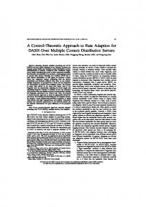
Navigation per definitionem includes the path planning and obeying of the chosen path while operating an arbitrary vehicle. The term ”navigation” deduces from the Latin words navis agere which means as much as operating a ship. The first who made use of so called navigation algorithms indeed were captains of ships when they planned and followed their routes over the sea. This was done using the method of dead reckoning, i.e. the distinction of velocity in magnitude and course. A route was planned by selecting some straight lines of constant course in an adequate map. The length of this lines describes the distance to travel before a new course has to be adjusted. This method builds the starting point of the evolution shown in Figure 1.1. The system knowledge has not to be very sound but also the level of plausibility or integrity is not the highest. This means by only measuring velocity and course of a vehicle one can not really rely on the calculated position when moving for a certain amount of time. In a next step velocity and course sensors have been replaced by sensors which measure accelerations and rotational rates between any two coordinate system. Here, two different methods have to be distinguished: Stabilized platforms are mechanical gimbaled platforms. The outer part of a stabilized platform is mounted fix to the vehicle while the inner part (the platform) can rotate freely around all three axis of a Cartesian coordinate system. Initially the inner part is aligned to the coordinate system where the navigation calculation takes place. Most often this is a local north pointing coordinate system. A rotating mass in the innermost frame holds this frame in it’s initial position due to gyroscopic counteracting torques, when trying to rotate the inner frame out of it’s position. Actuators and angular sensors on every hinge hold the inner platform always in it’s initial position. The measurable angles between the axes describe the vehicles orientation and accelerations can simply be measured on the inner platform. Simple integration gives velocity and later on position in the reference coordinate system. Strap Down Algorithms (SDA) use an Inertial Measurement Unit (IMU) to measure accelerations and angular rates between the vehicle fixed sensor coordinate system and the inertial
1
1 Motivation and Evolution of Navigation Plausibility/ Integrity Own Approach (complete breakup of model and reality)
INS with model constraints
Inertial Navigation Systems (INS) Dead Reckoning (Integration of velocity)
Algorithmic complexity
Figure 1.1: Evolution of navigation systems from the former dead reckoning algorithms to model based approaches in the last decade.
reference system. The SDA is the mathematical counterpart of a stabilized platform. The stabilization is realized by integration of the rates to an orientation matrix which transforms the body fixed accelerations to accelerations expressed in a certain coordinate system. In contrast to stabilized platforms these kind of assembly is very prone to sensor errors which result in a distinct drift over time. Without any aiding in terms of absolute sensors (such as position or heading) these Inertial Navigation Systems (INS) can provide a good solution only for a few minutes depending on the sensors accuracy. But due to the high frequency measurements of these inertial sensors, typically about 100 Hz, one has a quasi continuous solution for position, velocity and attitude of the vehicle. A comprehensive description of the incorporated mathematics is given for example in [Bri71, TW97, Wen07]. In these references additional formulae to cope with numerous integration errors in computer based systems are given. These additional knowledge includes error effects of coning, sculling and serial calculation of parallel processes to mention a few. Many publications can be found which describe improvements of the used algorithms, [Bor71, Pit03, Sav06, CMC07, CL10]. Most of the improvements concern on the attitude estimation accuracy. This thesis does not make use of these high sophisticated algorithms as the main goal is to show the principal architecture of navigation systems. Using more sophisticated algorithms (Integrated Navigation Systems, INS with additional aiding sensors) made it possible to get a higher integrity of navigational data for the sake of more system knowledge and more expensive equipment. Further improvements were made
2
starting in the late 1990s and going further onward when incorporating some kind of vehicle constraints or rather complete vehicle dynamics [BS04, DSNDW01, HBH08, JDW03, VSO06, VSOG10]. In this thesis a new interpretation of navigation, flight dynamics and reasons for a certain movement is proposed. It results in a higher integrity and plausibility of navigational data while not needing more knowledge of the systems dynamical behaviour than the former approaches. Figure 1.1 classifies this new algorithm in contrast to the other solutions with respect to complexity and integrity. In current and past research on navigational systems, vehicle kinematics have not been taken into account in all extend. Most often it was assumed that measured accelerations and rotational rates are the reason for an arbitrary object to move. But what really induces a rigid body to translate and rotate are externally acting forces and torques. These quantities may be produced by a propulsion system, wind drag or any other source acting on the body. As Newton said, a bodies translational movement (i.e. its acceleration a) is caused by the sum of all acting forces F divided by the mass m: a=
1 F m
Rotational movement is induced by moments acting on a rigid body: ω˙ = J−1 · M where J is the vehicles inertia. Therefore it cannot be assumed that measured accelerations and rotational rates are the reason for a body to move. They can be measured because of the movement. This work will pursuit this dogma and tries to give a comprehensive description of a rigid bodies movement in three dimensional space. Section 1.1 gives a short introduction to the mode of operation of almost all common integrated navigation systems (i.e. INS with some kind of aiding sensors). To overcome some inherent drawbacks of such systems, especially when using low-cost sensors, so called modelbased algorithms came up, see [VSOG10] and references therein. A short introduction to this type of algorithm is given in section 1.2. Although there has been some work on this type of navigation algorithms a complete and desirable partition between model knowledge (i.e. the algorithms used) and reality (i.e. the real moving vehicle) has not been realized in all extend. Based on the resultant drawbacks a new extension of the navigational algorithm arose which represents the main part of this thesis. Section 1.3 gives the main ideas behind this new kind of navigation system based on a complete disjunction between reality and model. Therefore the essential steps for such a complete disjunction are explained. This results in a very easy and clear description of any motion in space. The chosen approach makes it possible to use any desired sensor for aiding the navigation algorithm. Also an easy parametrization of the incorporated Kalman filter is possible. It should be feasible to use very simple types of Kalman filters or Luenberger observers to filter the measured variables and estimate the missing. The adaptation of the algorithms behaviour to any desired purpose is easily possible by changing only single parts of it. Actually only the modelling of actuators and sensors needs
3
1 Motivation and Evolution of Navigation to be changed as will be explained later on. The algorithmic architecture always remains the same except for different parametrization depending on the specific purpose.
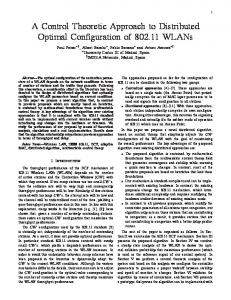
1.1 Conventional Inertial Navigation Systems (INS) Since the rise of miniaturized and powerful micro-controllers the former used mechanical platforms were replaced by so called Strap-Down algorithms which are a mathematical formulation of the gimbaled system. When looking at Figure 1.2 one can see the basic connections for an Integrated Navigation System (INS) with inertial and aiding sensors installed in an arbitrary vehicle. The vehicles motion is influenced by an input vector u, for example rudder deflections, thrust, flaps, etc. in an aircraft. The resulting motion can be measured through inertial sensors (accelerometers and gyroscopes) and also through aiding sensors, such as GPS, barometer or magnetometer to mention a few. The inertially measured data abib and ω bib are then fed into a Strap Down Algorithm (SDA) which transforms these variables into data useful for navigational purposes, i.e. position and velocity in an appropriate coordinate system and the vehicles attitude relative to a local north pointing tangential plane. In an aerospace context this is usually done using the Euler angels within the so called aerospace sequence [Kui02, p. 84ff.]. The SDAs output and the aiding data are fed into a Kalman filter to estimate the SDAs errors which are corrected in a further step. There are numerous descriptions of INS in the literature which are expanded by many different parts. These are for example coning and sculling corrections, different sample speeds inside the SDA amongst others. Good introduction but also comprehensive reference books are [Bri71, TW97, Wen07]. The description of all mentioned and assessed algorithms in this work is therefore rather short and concerns on the crucial parts of each algorithms while not being as comprehensive as the cited literature. But the basic mode of operation for every single algorithm should become obvious. Advantages While only using measurable inertial variables as input quantity, a conventional INS implementation can be used by just installing it in any vehicle without any adaptation. Depending on the modelled sensors aiding of the algorithm can be achieved easily. Drawbacks The whole algorithm can only work well when there are very good inertial sensors in use otherwise the integration of disturbed signals inside the SDA will lead to an undesired drift behaviour of the algorithm. The basic assumptions for Kalman filtering are also not met, when inaccurate sensors are used. Besides it is thought that all coordinate transformations inside the SDA are part of the reality. But essentially all transformations and calculations are only some kind of model of the reality. This circumstances motivate to put all calculations inside one single mathematical description of the real world which is explained in more detail later on. A more detailed description of such a navigation algorithm can be found in section 3. In this work it is referenced to as measurement model due to its special character of only transforming variables from one to another coordinate system. A high level block diagram
4
1.2 Conventional Model-based Approaches Reality u
Real Vehicles Movement
Inertial Sensors
Aiding Sensors
abib , ω bib SDA
δx
pe , v n
peSDA , v nSDA , q Kalman filter
ˆe, v ˆn, q ˆ p
Figure 1.2: Conventional Strap-Down (SDA) implementation of an Integrated Navigation System (INS) with aiding sensors for position and velocity updates. for this kind of Inertial Navigation System (INS) implementation is given in Figure 1.2.
1.2 Conventional Model-based Approaches Another type of solution to the basic navigation problem is formed by so called model based approaches. Here the separation into algorithms based on external (ExVD) or embedded vehicle dynamics (EmVD) is used, which was pointed out by [VSOG10] and references therein. All of these algorithms have been invented in the late 1990s and are still under development as recently published papers show. The next paragraphs give a short overview on the basic differences between ExVD and EmVD. Details are given in the respective sources cited.
1.2.1 External Vehicle Dynamics (ExVD) These algorithms were mentioned by different authors all around the world, i.e. [BS04, DSNDW01, HBH08, JDW03, KBI99, MSK03] and the development started in the late nineties of the last century. As can be seen in Figure 1.3 the SDA implemented in these model based solutions is used to provide position, velocity and attitude (like a normal sensor) of a vehicle, while aiding sensors are also used to provide some of these quantities. A parallel running vehicle dynamics block calculates also navigational data and therefore acts as another sensor for these quantities. Its structure has much similarity to a Luenberger observer but in detail it has some differences. With the help of a Kalman filter both the SDA and the vehicle dy-
5
1 Motivation and Evolution of Navigation Reality u
Real Vehicles Movement
Inertial Sensors
Aiding Sensors
abib , ω bib SDA
pe , v n
δx
peSDA , v nSDA , q Kalman filter ˆ bnb , v ˆ bnb , q ˆ ω
ˆe, v ˆn, q ˆ p
ˆ bnb , δˆ δω v bnb , δˆ q
Vehicle Dynamics
Figure 1.3: Model based navigation system with External Vehicle Dynamics (ExVD) and correction terms for the SDA and vehicle states. namics block are corrected by means of the residual between the aiding sensors quantities and the ones from the other sensors. Besides there use as additional sensors both the SDA and the vehicle dynamics block are not included in any further algorithm to improve the overall performance.
1.2.2 Embedded Vehicle Dynamics (EmVD) This kind of algorithm is a further development of the ExVD which was found by [VOS05, VSO06, VSOG10]. It has less system states compared to the ExVD for the sake of being more difficult to implement. Besides other drawbacks extensive transformations of system states need to be made. Figure 1.4 shows a block diagram of this algorithm. As for the ExVD algorithm a SDA is calculating the navigational data while aiding sensors provide additional quantities such as position and velocity measured by a GNSS. In contrast to the ExVD algorithm the vehicle dynamics are part of the Kalman filter’s internal model. Differences between the state estimates and the values from the aiding sensors are fed back into the SDA through a Kalman filter. Like already stated for the ExVD algorithm, vehicle dynamics and SDA serve as additional sensors and not as deterministic systems which they basically are.
6
1.3 Model Based Navigation System (FSVD) But the similarity between the EmVD approach and a Luenberger observer becomes more apparent than for the ExVD. Reality u
Real Vehicles Movement
Inertial Sensors
Aiding Sensors
abib , ω bib SDA
δx
pe , v n
peSDA , v nSDA , q Kalman filter & Vehicle Dynamics
ˆ bib , p ˆe, v ˆn, q ˆ ω
Figure 1.4: Model based navigation system with Embedded Vehicle Dynamics (EmVD) and correction terms for the SDA states.
Advantages Through the use of different kinds of sensors, i.e. vehicle dynamics and SDA, to provide the same quantities, some kind of analytic redundancy is achieved. The correction of both the vehicle dynamics as well as the SDA states provides a better navigation solution than only one of these system parts could provide. Especially drifting of the solution when no aiding sensors are apparent can be diminished. As proposed in the before cited sources, model based prediction of states can outperform conventional solution. Especially when low quality sensors are used, these approaches will lead to better results of the overall estimation performance. Drawbacks But there are also some major drawbacks of these solutions which become manifest in the incomplete breakup of reality and model. This will lead us to the afterwards mentioned new approach for hybrid navigation systems.
1.3 Model Based Navigation System (FSVD) Apart from all before mentioned approaches the new proposed algorithm will handle real measurements as measurements without any preprocessing or calculation. Predicted states
7
1 Motivation and Evolution of Navigation are handled as states. Measurements (Upper block in Figure 1.5) and model description (Bottom block in Figure 1.5) are completely divided and running in parallel as it is mandatory for observer based filtering structures. To the authors knowledge this is the first time that a complete breakup between reality and model has been realized for navigation algorithms. The so called observer structure has been realized in this new architecture to the full extend. While doing so, Kalman’s assumptions [Kal60] are kept in a most stringent way which is not always true for the other mentioned approaches. The vehicle model calculates all system states which are updated through arbitrary measurements, i.e. accelerometers, gyroscopes, GNSS, odometer, barometer or magnetometer to mention the primary ones. Besides its beauty and simplicity this algorithm also has the advantage of serving some kind of analytic redundancy. The output of the algorithm (i.e. all system states and some further variables) is always best fitted to the measured data up to its inherent model constraints. If a measured variable or a system state vary more than expected from a certain value a failure detection and isolation (FDI) could be run. Erroneous measurements or system states can be identified easily without any further extension of the algorithm. In coherence to other algorithm classification schemes the proposed one will be referred to as Reality u
Real Vehicles Movement
Inertial Sensors abib , ω bib
Aiding Sensors pe , v n
Kalman filter, Vehicle Dynamics, SDA & Sensor Models
ˆ bib , ω ˆ bib , a e ˆ ,v ˆn, q ˆ p
Figure 1.5: Approach for a new kind of model based navigation system (FSVD) with embedded vehicle dynamics, sensor models and strap down equations. an system which is working in a ”closed loop” mode (compare [BW10]) and predicting the full system state. Therefore the name Full State Vehicle Dynamics (FSVD) is introduced. As has been shown this full state or total state formulation bears some major advantages over the formerly introduced error state description (compare [WST00]). The following list illustrates the advantages of the new algorithm. In the next chapters the mathematical foundations and justifications for these advantages are given. 1. Precise prediction of all system states through • Modelling of all main influencing factors on systems dynamic behaviour
8
1.3 Model Based Navigation System (FSVD) • Accurate modelling of sensor behaviour • Coordinate transformations are made with predicted (and therefore smoother) variables • Measured values are not transformed but handled with all influencing disturbances 2. The core algorithm must not be changed depending on the application • Mathematical description of motion is always the same • Only actuator models need to be changed according to the specific purpose • Sensor models can be chosen and parametrized due to given methods Advantages To pre-record, before the implementation and validation of the new algorithm is explained, some major advantages are given here in advance. • Through the use of dedicated identification and estimation algorithms an easier parametrization of the complete algorithm is possible. • The stability of the overall estimation process can be guaranteed for convenient system excitations. • Knowing more about the complete system a better estimation of disturbances is possible. • When running in an unaided mode the proposed algorithm does not have the distinct drift behaviour of conventional solutions. • A very easy augmentation of the state vector is assured. This makes a further use for Failure Detection and Isolation (FDI) possible easily.
Drawbacks Beside the clear advantages of the proposed algorithm there are also some major drawbacks which will be shortly addressed in the following list: • More complexity of the algorithm in contrast to a conventional INS solution • Extensive identification and parametrization procedures have to take place • In contrast to the INS/GPS combination there is no plug and play possible when attaching the algorithm to a new technical system. • When using high-end sensors model based approaches do not have any great advantages.
9
1 Motivation and Evolution of Navigation
1.4 Structure of this work The next chapter concerns on the description of the investigated navigation algorithms. It starts with the state of the art SDA based algorithm in section 1.1 and continues with the description of other model based algorithms in section 2.3 and section 2.4. The mathematical foundations for the later assessment are laid as well as the principal mode of operation of the different algorithms. Chapter 3 introduces the main contribution of this work: the description of the Full State Vehicle Dynamics (FSVD) algorithm. The mathematical system modelling is repeated shortly and the setup of the navigation filter (Kalman filter) is described. All further investigations are based on any 6 degrees of freedom motion in space. In chapter 4 as well as in the appendix the principal mathematics are explained for any movement between different coordinate systems. The next sections of chapter 4 describe the modelling of the two assessed systems. On the one hand a quadrotor simulation model is described in section 4.2 and on the other hand the example of a navigation test vehicle (NavBus) is given in section 4.3. The NavBus has different high-end but also low-cost sensors on board an deals as test vehicle to compare different approaches with each other. In this thesis the high-end IMU serves as a reference whereas the low-cost sensors serve as measurement system for the new model based navigation algorithm. In a last step the used sensors are described from a deterministic as well as a stochastic point of view in section 4.4 Having set up a complete system description with encapsulated models of the vehicle, sensors and navigational calculations, simulations as well as measurement campaigns have been performed to analyse and validate the new approach. A description of the simulation environment and results can be found in chapter 5. In a next section a real measurement campaign with the NavBus has been performed and analysed. Results are given in the respective sections. In the last chapter a summary is given. Some limiting factors and an outlook for further improvement are also given in chapter 6. The appendix enlightens the different coordinate systems used in this work and how variables are identified uniquely. Also some signal processing fundamentals just as well as the theory behind Kalman filters will be clarified in this chapter.
10
2 Conventional and Model Based Navigation Algorithms The different navigation architectures assessed in this thesis are introduced in the following. Inertial Navigation Systems (INS) are described in full state formulation in section 2.1 and in error state formulation in section 2.2. These two approaches are commonly used in inertial navigation systems. While the full state formulation is most often used in combination with low cost sensors, the error state formulation is used with high end sensors. The last sections describe model based approaches which were invented in the late 1990s and early 2000s by different researchers. All model based algorithms have in common the error state formulation of an INS. The new proposed algorithm, which is described in chapter 3 relies on the full or total state space formulation like it is described for example in [WST00, WST01].
2.1 Full State Inertial Navigation System (FS-INS) ˆ k−1 x
z −1
ˆ− x k
ak , ω k
Prediction � � �� ak ˆ− ˆ x = f x , k−1 k SDA ωk
P− k
=
Fk Pk−1 FT k
+
Gk QGT k
P− k
Correction � �−1 T − T Kk = P− k Hk HPk Hk + R �� ˆk = x ˆ− ˆ− x k + Kk y − h x k Pk = (I − Kk Hk ) P− k
yk
Pk−1
ˆk x
Pk
z −1
Figure 2.1: Kalman filter architecture for the use of a full state SDA based algorithm. For comparison purposes a full state based SDA algorithm has also been implemented according to equations (2.1). It calculates position changes in a local levelled Cartesian coordinate system, whereas velocity is expressed in a body fixed coordinate system. The orientation is expressed using quaternions in Equation 2.1c. Because sensor errors such as
11
2 Conventional and Model Based Navigation Algorithms bias are always apparent these quantities can be estimated online using a so called random walk approach (i.e. b˙ = 0) in equations (2.1d) and (2.1e). p˙ n = Cnb v b v˙ b = a q˙ =
"
(2.1a) #
1 0 −ω T · q. 2 ω −Ω
b˙ a = 0 b˙ ω = 0
(2.1b) (2.1c) (2.1d) (2.1e)
Where a and ω are the effective quantities which result in the vehicles movement. These ideal values can only be measured with errors such as bias ba,ω and noise na,ω which leads to the measurable quantities abib = a + ba + Cbn g ne + na
(2.2)
ω bib = ω + bω + nω .
(2.3)
For the sake of simplicity additional effects such as g-force uncertainties and Earth rotational effects are neglected in abib and ω bib . After subtracting the biases and g-force from abib and ω bib the effective accelerations a and rotational rates ω are given through: a = abib − ba − Cbn g ne
ω=
ω bib
− bω .
(2.4) (2.5)
which are then fed into equations (2.1) to give an estimate of the state vector x iT h �T x = (pn )T , v b , (q)T , (ba )T , (bω )T
(2.6)
The here mentioned formula are only used inside the Strap-Down Algorithm (SDA), the External (ExVD) and Embedded Vehicle Dynamics (EmVD) approaches for the prediction of the vehicles movement which can be seen in figures 1.2, 1.3 and 1.4. Inside the corresponding Kalman filters an error state formulation of the Strap-Down algorithm is used which will be explained in the next section.
2.2 Error State Inertial Navigation System (ES-INS) The EmVD as well as the ExVD approach have in common the error state formulation of the Strap-Down Algorithm (SDA) which calculates the errors in position pn , velocity v b and attitude q of any arbitrary vehicle according to equations (2.1). These equations are used inside the prediction step of the model based algorithms to have an estimate of the actual state. The correction step corrects the misleading predicting estimate by the use of aiding measurements. Therefore an linearized error model of the differential equations needs to be set
12
2.2 Error State Inertial Navigation System (ES-INS) ˆ SDA,k−1 x
-
z −1
Pk−1
Error Prediction
ak , ω k
SDA Prediction
ˆ− δx k
ˆ− x SDA,k
=0
T T P− k = Fk Pk−1 Fk + Gk QGk
Measurement residual
z −1
ˆ− δx k P− k
Error Correction � �−1 T − T Kk = P− k Hk HPk Hk + R
ˆk δx
ˆ k = Kk δy k δx ˆk δy
ˆk = y − x ˆ− δy SDA,k
yk
Pk
Pk = (I − Kk Hk ) P− k
Figure 2.2: Kalman filter architecture for the use of an error state SDA based algorithm. up. Building the partial derivatives of (2.1) results in equations (2.7) under the assumption of zero mean white noise n which is additive to all system states. δ p˙
n
δ v˙ b δ q˙
� ∂ Cnb v b δq = + ∂q � ∂ Cbn g ne = −δba + δq ∂q 1 = − WT δbω 2 =0 Cnb δv b
δ b˙ a δ b˙ ω = 0
(2.7a) (2.7b) (2.7c) (2.7d) (2.7e)
where W is the Jacobian −q1 q0 q3 −q2 ∂ q˙ W =2· = −q2 −q3 q0 q1 ∂ω −q3 q2 −q1 q0 The state vector for the Kalman filter is given by the left hand sides of equations (2.7): h iT �T δx = (δpn )T , δv b , (δq)T , (δba )T , (δbω )T
(2.8)
2.2.1 Implementation ˆ is set For the implementation of an error state INS an EKF with the error state vector δ x up. The prediction step is given through: � � T ˆ− ˆ δx = f 0, [a , ω , x ] + GnxINS k k INS,k k T T P− k = FPk−1 F + Gk QGk
(2.9) (2.10)
13
2 Conventional and Model Based Navigation Algorithms where the matrix F is the Jacobian of f with respect to δx and G is the influence matrix ˆ INS,k is calculated using of the assumed white noise nINS acting on δx. The state vector x equations (2.1) with the current inertial quantities and the state vector from the last time step. The Kalman gain can be calculated through: − T T Kk = P− k Hk · Hk P k Hk + R
�−1
(2.11)
with the measurement Jacobian Hk . For the state update of δx and also the covariance update to following equations are used: ˆ k = Kk (y k − h (ˆ δx xk−1 )) Pk = (I −
(2.12)
Kk Hk ) P− k
(2.13)
ˆ k is updated through x ˆk = x ˆ k−1 + δ x ˆ k−1 and the error For the next step the state vector x ˆ k−1 = 0 afterwards. The above used matrices and vectors are given by the state is set to δ x following expressions. For the sake of simplicity and readability the index ()INS is omitted in all formula. For a later distinction these indices are crucial. n b n n ∂ (Cb v ) 0 0 np δˆ p ∂q 0 Cb b gn b δˆ ∂ C ( ) n e 0 0 nv v −I 0 ∂q ˆ = δˆ FINS = 0 0 (2.14) δx q , nxINS = nω 1 T 0 0 − W 2 ˆa nba δb 0 0 0 0 0 ˆω nbω δb 0 0 0 0 0 2 I 0 0 0 0 0 0 σp 0 0 0 σ2 0 0 0 0 0 0 0 I a GINS = 0 0 − 21 · WT 0 0 (2.15) QINS = 0 0 σ 2ω 0 0 2 0 0 0 0 0 σ ba 0 0 −I 0 0
0
0
0
σ 2bω
0 0
0
0
−I
Inside the matrix Q uncorrelated noise on every state is assumed. It is numerical zero for the position variance σ p . The noise variance of the inertial sensors is directly written into the terms σ a and σ ω . To have a smooth but reactive bias estimation possibility the values for σ ba and σ bω are set to roughly one tenth of the inertial sensor noise parameters. This enables the Kalman filter to both estimate the initial offset but also follow a slowly drifting mean value of the signal.
2.3 External Vehicle Dynamics (ExVD) The aiding of a SDA navigation solution with a vehicle dynamics model can be achieved in many different ways. Different researchers have proposed solutions to optimally fuse data from various sensors and models, [BS04, DSNDW01, HBH08, JDW03, VSO06, VSOG10]. Here the External Vehicle Dynamics (ExVD) formulation by Vasconcelos et al, [VSO06, VSOG10], is described. This architecture was proposed first by Koifman an Bar-Itzhack in 1999, [KBI99],
14
2.3 External Vehicle Dynamics (ExVD) ˆ SDA,k−1 x
-
z −1
Pk−1
z −1
ˆ− δx k SDA Prediction
ak , ω k uk
VD Prediction
ˆ− x SDA,k
Error Prediction � � − �� ˆ SDA,k x ˆ− δx − k = f ExVD 0, ˆ VD,k x P− k
ˆ− x VD,k
=
Fk Pk−1 FT k
+
P− k
Gk QGT k
Pk Error Correction � �−1 − T T Kk = Pk Hk HP− k Hk + R � � − �� ˆ ˆ k = δx ˆ− δx k + Kk δy − h δxk
ˆ SDA,k δx
Pk = (I − Kk Hk ) P− k
Measurement residual
ˆ VD,k δx
ˆk δy
yk
ˆ VD,k−1 x
z −1
-
Figure 2.3: Kalman filter architecture for the use of the ExVD based algorithm. while Vasconcelos has made the attempt to describe all model based algorithms in a consistent way. As can be seen in Figure 1.3 the vehicle dynamics (VD) model serves as one more sensor for the quantities which can also be calculated through a SDA. Input into the VD algorithm are the control inputs to the vehicle. They are produced either by an operator or controller. The outputs of the SDA and VD algorithms are the inputs of the Error Prediction algorithm as well as the Measurement Residual calculation, where also real measurements are taken into account. The Error Correction block fuses the measurement residuals and predicted errors ˆ VD and δ x ˆ SDA which are fed with an Extended Kalman filter and outputs correction terms δ x ˆ SDA back to correct the prediction of the respective states. After each time step the error δ x is set to zero. Inside the SDA Prediction block the SDA states are predicted with equations (2.1). The dynamical behaviour of the motors as well as of the flight dynamics are modelled according to chapter 4 and result in the following differential equations, which are calculated inside the VD Prediction block: Cw b b F bM + Cbn g ne − ω bnb × v bnb − v v m nb nb m � b T 1 0 − ω nb fq = ·q 2 b ω nb −Ω � � fω = J−1 M bM − Cm · ω bnb ω bnb − ω bnb × Jω bnb fv = −
fxA = f (xA , u)
(2.16a) (2.16b) (2.16c) (2.16d)
The specific forces F bM and torques M bM are produced through the actuators installed in the arbitrary vehicle. In contrast to the vehicle dynamics models mentioned by i.e. [BS04,
15
2 Conventional and Model Based Navigation Algorithms DSNDW01, HBH08, KBI99, VSO06, VSOG10] the vehicle dynamics model block is expanded by the differential equations which describes the motor speed dynamics in Equation 2.16d. Former model based approaches usually rely on acting forces and moments as input quantities which are provided by an arbitrary propulsion system. Here, the propulsion system is included into the vehicle dynamics model without loss of generality. The derivation of all derivatives and matrices is omitted here but [VSOG10] and references therein provide the basics for all following equations and matrix structures. With the partial derivatives of equations (2.16) the error state formulation of the vehicle dynamics model is:
δ ω˙ VD = δ v˙ VD = δ q˙ VD = δ x˙ A,VD =
∂fω δω VD ∂ω xVD ∂fv δω VD ∂ω xVD ∂fq δω VD ∂ω xVD ∂fxA δω VD ∂ω xVD
∂fω + δv VD ∂v xVD ∂fv ∂fv + δv VD + δq ∂v xVD ∂q xVD VD ∂fq + δq ∂q xVD VD ∂fxA + δv VD ∂v xVD
∂fω + δxA,VD ∂xA xVD ∂fv + δxA,VD ∂xA
(2.17a) (2.17b)
xVD
∂fxA + δxA,VD ∂xA xVD
(2.17c) (2.17d)
The index ()VD shows that for the calculation of these quantities only states from the vehicle dynamics model are used. The calculation of SDA and VD states is completely independent of each other and therefore almost every state is calculated twice. The ExVD block serves as additional sensor for the Kalman filter.
2.3.1 Implementation The implementation of the Kalman filter consists of two steps. First an augmented state vector xC is created. It includes both the inertial estimates xINS and the vehicle dynamics estimates xVD . "
# " # ˆ INS δx nxINS ˆC = , nxC = , δx ˆ VD δx nxVD " # QINS 0 QC = , 0 QVD
"
# FINS 0 FC = 0 FVD " # GINS 0 GC = 0 GVD
(2.18) (2.19)
Due to the parallel processing of INS and VD estimates the system dynamics can be expressed as block diagonal matrices which are given through FC , QC and GC . The Kalman filter still has the same mode of operation as described for the error state INS in the section before.
16
2.3 External Vehicle Dynamics (ExVD) The new sub matrices and vectors for the vehicle dynamics are given through:
ˆ VD δx
ˆ VD δω δˆ v VD = δˆ q VD ˆ A,VD δx
,
nxVD
nωVD nv VD = nqVD nxA,VD
,
FVD
=
∂fω ∂ω
∂fω ∂v
0
∂fω ∂xA
∂fv ∂ω
∂fv ∂v
∂fv ∂q
∂fv ∂xA
∂fq ∂ω
0
∂fq ∂q
0
∂fxA ∂ω
∂fxA ∂v
0
∂fxA ∂xA
(2.20)
The transformation-matrix and process noise covariance matrix are given through. These are simple diagonal block matrices as for the INS covariances. A correlation between different states is achieved through the system matrix F.
GVD
=
I 0 0 0
0 0 I 0 1 0 − 2 WT 0 0
0 0 0 I
,
QVD
=
0 0 0 σ 2ωVD 2 0 0 0 σ vVD 2 0 0 0 σ qVD 2 0 0 0 σ xA,VD
(2.21)
These equations directly show the high computational load which is necessary to solve for all variables. Not only the full INS state vector needs to be estimated but also the complete VD vector which consists of at least 10 states, when no additional actuator states are included. A total of 26 states therefore needs to be calculated each prediction step. Measurements for the correction of both the INS and VD states are obtained straight forward by a simple subtraction of corresponding states which is given through the matrix HVD . This matrix is build up as the Jacobian of δz VD with respect to the augmented state vector xC .
δz ω = ω − ω VD − bω
(2.22a)
δz v = v SDA − v VD
(2.22b)
δz xA = xA − xA,VD
(2.22d)
δz q = q SDA − q VD
(2.22c)
17
2 Conventional and Model Based Navigation Algorithms With the expressions
δz VD =
RVD =
HVD (xINS ) =
nω + nzω nzv , n = z VD nzq nzxA σ 2ω + σ 2zω 0 0 0 0 0 σ 2zω 0 0 0 σ 2zq 0 0 0 0 σ 2zxA
δz ω δz v δz q δz xA
0 0 0 0
0 I 0 0
0 0 I 0
0 −I −I 0 0 0 0 0 0 −I 0 0 0 0 0 0 −I 0 0 0 0 0 0 −I
(2.23)
(2.24)
(2.25)
which are used inside the Kalman filters update step. The block diagonal structure of all involved matrices is still apparent. Correlation between states, and therefore better estimation possibility and observability are only achieved through FVD . This motivated [VSO06, VSOG10] to change the architecture of the model based algorithm which they call Embedded vehicle dynamics. They wanted to gain the same estimation performance by using only parts of the parallel running vehicle dynamics and INS estimates. A short formulation of the result is given in the next section whereas a comprehensive derivation of all formula can be found in the before mentioned papers.
2.4 Embedded Vehicle Dynamics (EmVD) The goal of Vasconcelos et at. [VSO06] was to achieve the same performance as the ExVD approach without predicting the whole state vector twice, once in the SDA and once in the VD block. Vasconcelos therefore designed the algorithm structure which is shown in Figure 2.4. The SDA estimates serve as an input to the Measurement Residual and the Error-State Prediction block. The reformulation of the vehicle dynamics using the SDA estimates results in the following system of differential equations. They are based on the partial derivatives of equations (2.16): ∂fv ∂fv ∂fv b δbω − δv − δq (2.26a) v˙ VD = fv + ∂ω xINS ∂v xINS ∂q xINS ∂fω ∂fω ω˙ VD = fω + δbω − δv b (2.26b) ∂ω xINS ∂v xINS ∂fxA ∂fxA x˙ A,VD = fxA + δbω − δv b (2.26c) ∂ω xINS ∂v xINS The terms fv , fω and fxA are solved using the input voltages to the motors and the SDA state estimates. The calculation is done completely inside the Error-State Prediction block, which
18
2.4 Embedded Vehicle Dynamics (EmVD) ˆ SDA,k−1 x
z −1
Pk−1
ak , ω k
ˆ− x SDA,k
SDA Prediction
uk
Error-/State Prediction − � � ˆ SDA,k x ˆ− δx k = f EmVD 0, x ˆ VD,k−1 − ˆ VD,k x uk T T P− k = Fk Pk−1 Fk + Gk QGk
Measurement residual
z −1
Pk ˆ− δx k P− k ˆk ω
Error-/State Correction � �−1 T − T Kk = P− k Hk HPk Hk + Rk � � − �� ˆ ˆ k = δx ˆ− δx k + Kk δy − h δxk
ˆ SDA,k δx
Pk = (I − Kk Hk ) P− k
ˆ VD,k x
ˆk δy
yk
ˆ VD,k−1 x
z −1
Figure 2.4: Kalman filter architecture for the use of the EmVD based algorithm. induced Vasconcelos to call in Embedded Vehicle Dynamics. With some more reformulation it is also possible to exclude the calculation of v˙ VD in the prediction step of the algorithm which is shown in [VSOG10]. But the included reformulation of all involved equations is extensive and very prone to errors if the prediction of additional states such as motor speed is needed. Inside this thesis the simpler but slower (in terms of calculation time) version is used. As can be seen in Equation 2.26 the prediction of the vehicles attitude is excluded inside the VD algorithm. Only the equations which relate forces and torques to changes in translational and rotational velocity are calculated. Additional the prediction of the motor speed is included, because the input forces and moments are not known directly as assumed by [VSOG10] and references therein. The measurement equations are: � � � � � � ∂fv ∂fv ∂fv ˆ a = ga = V − y · bω + Ω − · δv + Ω − · VWδq + ba (2.27a) ∂ω ∂v ∂v ˆ ω = gω = ω VD − bω y
ˆ xA = gxA = xA y
(2.27b)
(2.27c)
Herein V and Ω are given as the skew symmetric matrices: 0 −w v 0 −r q � � V = v bnb × = w Ω = ω bnb × = r 0 −u 0 −p −v u 0 −q p 0
2.4.1 Implementation Inside the embedded Kalman filter the state vector is also augmented and matrices are adapted accordingly. In contrast to the ExVD approach the matrices are no longer block diagonal ones
19
2 Conventional and Model Based Navigation Algorithms which introduces correlation between all steps without the high computational burden of an ExVD architecture. All partial derivatives are the same as in the the ExVD approach but they are estimated for the INS state vector and not for the VD state vector, which can be ˆ C is given in Equation 2.28 as well seen in Equation 2.26. The complete error state vector δ x as the noise terms nxC and the input vector uC . The structure of the state and covariance matrices can be seen in Equation 2.29. " # " # " # ˆ INS δx nxINS fw (x, u) ˆC = δx , nxC = , uC = (2.28) ˆ VD δx nxVD fv (x, u) " # " # " # FINS 0 QINS 0 GINS 0 FC = , QC = , GC = (2.29) FVD 0 0 QVD GVD I Like for the ExVD approach the submatrices FVD , GVD and H consist of the partial derivatives of the vehicle dynamics which are solved for the INS state estimate. ˆ VD δx
ω ˆ VD = ˆ VD v ˆ A,VD x
,
nxVD
nωVD = nvVD nxA,VD
,
FVD
0 − ∂fω ∂v ∂f = 0 − ∂vv ∂f 0 − ∂vxA
0
∂fω ∂ω
v − ∂f 0 ∂q
∂fv ∂ω
0
0
0
∂fxA ∂ω
(2.30) Due to the reformulation of the ExVD approach the calculations of the measurement residual matrix H becomes more complex than for the ExVD solution and also the measurement covariance matrix needs to be calculated every time step using the actual system states, which can be seen in Equation 2.33. Nevertheless the computational load can be decreased quite well, which has been shown in [VSOG10] and is also mentioned in section 5.2. GVD
0 0 − ∂fω ∂ω ∂f = 0 0 − ∂ωv ∂fxA 0 0 − ∂ω
0 H= 0 0
0 0 0 0 , 0 0
0
∂ga ∂v
∂ga ∂q
I
∂ga ∂ω
0
0
0
0
where σ ∗ is given through σ 2∗
20
=
σ 2a
+
0 ∂ga , 0 ∂xA 0 I
0 −I I
0
QVD
�
σ 2ω 0 0 VD = σ 2vVD 0 0 0 0 σ 2xA,VD
σ 2ω + σ 2zω 0 0 R= 0 σ 2∗ 0 0 0 σ 2xA
� � �T ∂fω ∂fω 2 − V σω −V + σ 2zv ∂ω ∂ω
(2.31)
(2.32)
(2.33)
2.4 Embedded Vehicle Dynamics (EmVD) In contrast to the ExVD architecture the correlation between states is achieved through the block diagonal matrix R which has been a pure diagonal matrix for the ExVD. The calculation of FVD therefore is a bit simplified due to neglecting the VD estimates for the prediction of the full state vector. As for the measurements correlation is introduced to a rather full matrix GC .
21
3 New Model Based Navigation Algorithm with Observer Structure This chapter enlightens the motivation for creating a new kind of model based navigation algorithms. In contrast to all before mentioned approaches the newly introduced Full State Vehicle Dynamics (FSVD) algorithm runs completely parallel to the reality which gives motivation to call it also observer structure of a model based navigation algorithm. Figure 3.1 shows the basic architecture which has been developed in order to have a completely parallel running model which is only fed by the input vector u. The output of the nonlinear actuators Reality Operator or Controller
u
Actuators
xA
Vehicle Dynamics
Specific Sensor
K
a, ω
vb n p q
Inertial Navigation
Inertial Sensors
Aiding Sensors
Specific Sensor Model
Model of Actuators
ˆA x
Inertial Sensor Models
Vehicle Dynamics Model
ˆ, ω ˆ a
Aiding Sensor Models
Strap Down Algorithm
b ˆ v n ˆ p ˆ q
Filter model
Figure 3.1: Observer based filter architecture which is used in combination with the FSVD based algorithm. can be the actuators state vector or any derived quantity. In contrast to the figure, which
23
3 New Model Based Navigation Algorithm with Observer Structure has been simplified, there are also the forces and torques available as output of the actuator block. These quantities serve as input to the flight mechanics block. The flight mechanics block transforms forces and torques into accelerations and rotational rates which can be measured by inertial sensors. In a last step the Strap-Down Algorithm transforms coordinate systems and integrates to inertial variables to get the complete state vector of the vehicle. The biggest advantage of observer based structures is that is is possible to calculate the complete state vector given only the input quantities. A failure detection of inertial sensors but also common aiding sensors is made possible also very easy. The distinction between inertial and aiding sensors is made here in conjunction with common literature to not be confused. But basically all sensors are considered as sensors and have their influence only in the update step of the Kalman filter. Prediction of the state vector is based solely on the input voltages to the motor which, in reality, are fed to the real motor and the mathematical model through the same interface. Kalmans assumption of a deterministic input which is only affected by white noise is therefore fulfilled.
3.1 Full State Vehicle Dynamics (FSVD) ˆ k−1 x
z −1
ˆ− x k Prediction uk
ˆ− x xk−1 , uk ) k = f FSVD (ˆ P− k
=
Fk Pk−1 FT k
+
Gk QGT k
P− k
Correction � �−1 T − T Kk = P− k Hk HPk Hk + R �� ˆ− ˆk = x ˆ− x k k + Kk y − h x Pk = (I − Kk Hk ) P− k
yk
Pk−1
ˆk x
Pk
z −1
Figure 3.2: Kalman filter architecture which is used in combination with the FSVD based algorithm. An overview of the new proposed full state model based navigation algorithm is given in Figure 3.2. As can be seen the basic architecture is the same as for the INS. The only but crucial difference is the handling of input and measurement data. Here only the voltages to the motors uk are given as input to the system while accelerations and rotational rates are handled as measurements y k . Inside the Prediction block the full state prediction according to equations (3.1) is done. The Correction block afterwards calculates the measurement residual as given in equations (3.3). This observer based approach can run completely parallel to reality
24
3.1 Full State Vehicle Dynamics (FSVD) without needing any measurements. The prediction is based solely on the input voltages. fp = Cnb v bnb
(3.1a)
F bM Cw b b + Cbn g ne − ω bnb × v bnb − v nb v nb m m � T 0 − ω bnb 1 fq = · q. 2 −Ω ω bnb
fv = −
(3.1b)
(3.1c)
fba = 0 fbω = 0
fω = J
−1
(3.1d) (3.1e)
� b � M M − Cm · ω bnb ω bnb − ω bnb × Jω bnb
(3.1f)
fxA = f (xA , u)
(3.1g)
The differential equations for the full state vector are then given through �T � x˙ = fpT , fvT , fqT , fbTa , fbTω , fωT , fxTA
(3.2)
The input vector u fed into equation (3.1g) is provided either by the operator or by a controller. To be comparable to the other introduced algorithms the measurement vector only consists of acceleration, rotational rate and the states of the actuation system. ˆ a = ga = fv − Cbn g ne + ba y
ˆ ω = gω = y
ω bnb
(3.3a)
+ bω
(3.3b)
ˆ xA = gxA = xA y
(3.3c)
3.1.1 Implementation For the implementation several vectors and matrices have to be set up. The state noise vector nx and covariance matrix are given by: ˆn p np σ2 0 0 0 0 0 p n 0 σ2 0 v b 0 0 0 ˆ v v qˆ n 0 0 σ2 0 0 0 q Φ 2 ˆ ˆ = x 0 ba , nx = nba , Q = 0 0 0 σ ba 0 b nb 0 0 0 ˆ 0 σ 2bω 0 ω ω ω nω 0 0 0 0 0 σ 2ω ˆ ˆA x
nxA
0
0
0
0
0
0
ˆ, state vector x
0
0 0 0 0 0 2 σ xA
(3.4)
ˆ because the covariance of a quaternion σ 2q The dimension of Q is smaller than that of x depends very much on the quaternion itself. To circumvent this the Euler angle variance σ 2Φ
25
3 New Model Based Navigation Algorithm with Observer Structure is used which is not dependent on the actual orientation. To increase the dimension of the resulting Q the original Q is multiplied from the left and right side by G and GT according q to Equation 18. With the term ∂f this increase is achieved for the Euler or quaternion ∂ω covariance. F=
0
∂fp ∂v
∂fp ∂q
0 0
0
0
0
∂fv ∂v
∂fv ∂q
0 0
∂fv ∂ω
∂fv ∂xA
0
0
∂fq ∂q
0 0
∂fq ∂ω
0
0
0
0
0 0
0
0
0
0
0
0 0
0
0
0
0
0
0 0
∂fω ∂ω
∂fω ∂xA
0
0
0
0 0
∂fxA ∂ω
∂fxA ∂xA
G=
I 0
0
0 I
0
0 0
∂fq ∂ω
0 0
0
0 0
0
0 0
0
0 0
0
0 0 0 0 0 0 0 0 0 0 0 0 I 0 0 0 0 I 0 0 0 0 I 0 0 0 0 I
(3.5)
For all other states being uncorrelated this transformation must not be made and therefore the remaining diagonal elements of Q are set to one. In contrast to the other model based approaches we now have a deterministic input which has an additional white noise which fully meets Kalmans assumptions. The variance of the white noise ΣA is added to the Covariance matrix P according to equation (3.6). T T T P− k = Fk Pk−1 F + Gk QQk + Bk ΣA Bk
(3.6)
where ΣA is a diagonal matrix with the noise variance of the input quantity: B=
�
0 0 0 0 0
0 H= 0 0
26
� ∂fω T ∂u
�
∂ga ∂xA
∂ga ∂v
0 I 0
∂ga ∂ω
0
0 0 I
I
0
0 0 0
0
∂fxA ∂u
0 I
�T
�T
2 σu1 0 0 σ2 u2 ΣA = . .. . . . 0 0
···
0 ··· 0 . .. .. . 2 · · · σum
2 0 σa 0 R= 0 0 σ 2ω 0 0 σ 2xA
(3.7)
(3.8)
4 Modelling of two Example Systems System modelling of any real physical controlled system coarsely can be divided into four different parts as can be seen in Figure 4.1. Basically a pilot or operator can influence a
w
e
Controller
u
Actuators
F /M
Rigid Body Motion
x
Sensors
y
Figure 4.1: Basic architecture of a control configured vehicle. A rigid body can be influenced via actuators and the resulting motion can be captured with sensors. technical system via a control demand w. A controller then calculates the input quantities for the actuators from the difference between demand and actual system state y. The systems behaviour can be measured with sensors and is fed back the controller. The following sections of this chapter will describe each single block in detail. While controller and actuators are specific for the used concrete test-bed the sensor description is independent of this. The Description of a rigid bodies movement in space is also independent of the assessed technical system. This motion can be described in many different ways. First one has to choose appropriate coordinate systems in which all calculations are expressed. The most commonly used systems are given in Figure 1. Besides there are many different ways to express the mathematics behind the rigid bodies movement. In this thesis a quaternion based attitude representation is chosen. Section 4.1 describes the quaternion based approach in a local north pointing system which is sufficient for small short range UAV. Translational movements are described using the well known laws of Newton. A rigid bodies movement is always the result of external acting forces and torques. With the systems mass and inertia these external excitation results in linear accelerations and rotations around the bodies principal axes. These resulting variables may be measured by inertial sensors such as accelerometers and gyroscopes. A quadrotor helicopter was chosen to be the analysed system. Also the institute of Flight Systems and Dynamic Control (FSR) has done quite much research on this kind of aircraft which makes it easy to get real flight data for further analysis of the different implemented navigation systems. In section 4.2 the mathematical description of the test platform is given. Depending on the aspects to be modelled there has been made the division into deterministic and stochastic system modelling. While the navigational part of the complete algorithm can be described very accurate by mathematical expression some influences of the actuators
27
4 Modelling of two Example Systems can be modelled easier by using a stochastic approach. The stochastic analysis is based on investigations of the Power Spectrum Density (PSD) which gives some deeper insight into disturbances caused by vibrations for example. The next part of this chapter concerns about Sensor modelling. It consists of the data transformation algorithms to get measurable variables from modelled ones in the first part. Furthermore subsection 4.4.2 deals with the stochastic description of sensors and explains how the parametrization of the resulting models is made. The controller used for trajectory and attitude control is described in the last part of this chapter. From a high-level point of view the principal structure and mode of operation is explained. Details are described in the following.
4.1 Rigid Body Motion Sometimes the kinematics of an arbitrary vehicle allow for manoeuvres that need the full range of angles. In this case the Euler angle based approach will lead to an unwanted behaviour when the pitch angle reaches ±90◦ . For this case heading angle ψ and roll angle φ fall into place and can not be distinguished any more. With rotation sequences described by quaternions (compare 1.3) this drawback can be eliminated. The following section describes a quaternion based rigid body motion for short distance movements of an UAV on a local level north pointing system. With some upgrading this can also be used for long distance travelling above a rotating Earth which is already described in section 3. Due to the inherent instability of the height channel an overall system instability arise which need to be treated separately. This is not part of this work - basically a controller with the barometric height as set point is used to control the SDA to not drift away with time [Aus91, WS80].
4.1.1 Movement in a Local North pointing Reference System Except for long range flights it is sufficient to calculate the vehicles movement in a local Cartesian coordinate system. This coordinate system has it’s origin at [0 0 0]T which initially coincides with the actual position on Earth, i.e. latitude, longitude and height. From the start point position is measured in meters in all three axis. Here the navigation coordinate system is used for this purpose. The calculations of motion therefore simplify to the expression given in Eqs. (4.1). p˙ n = Cnb v bnb Cw b b F bM + Cbn g ne − ω bnb × v bnb − v v m nb nb "m # �T 1 0 − ω bnb q˙ = · q. 2 ω bnb −Ω � � ω˙ bnb = J−1 M bM + M bbias − Cm · ω bnb ω bnb − ω bnb × Jω bnb v˙ bnb = −
28
(4.1a) (4.1b) (4.1c) (4.1d)
4.2 Quadrotor The Cnb Matrix is given by Equation 3 and transforms states from b-coordinates to ncoordinates. It is calculated from the actual quaternion in Equation 4.1c. A block diagram of the whole algorithm is given in Figure 4.2. The input u from pilot or operator produces the driving forces and moments which act on the vehicle. Additional bias moments are introduced to cope with different positions of centre of gravity and geometric centre of the vehicle. The sum of all driving forces and moments act on the vehicle and force it to move in a certain direction with a certain attitude. Aerodynamic forces and torques are also introduced for the comprehensive modelling of the overall system. Additional forces due to wind have not been taken into account, but the state vector could easily be augmented by that states. Using eqs. (4.1b) and (4.1c) it is possible to calculate velocity and attitude of the vehicle. A following simple integration and coordinate transformation results in a position of the vehicle. The attitude which is calculated using quaternions may be transformed to Euler angles for a better understanding. Therefore one may use Equation 11. u
� � b F˙ M = f F bM , u
� � v˙ bnb = f v bnb , ω bnb , F b
v bnb
vn
Cnb
Translation
R
0
˙ b M M
M bbias
�
� = f M bM , u
Driving forces and torques
F bd = f v bnb
R
pn
�
M bd = f ω bnb
�
Aerodynamic forces and torques � � ω˙ bnb = f ω bnb , v bnb , M b
ω bnb
q˙ = f q, ω bnb
�
q
Rotation Vehicle dynamics
Navigational calculations
Figure 4.2: Quaternion based description of motion for a local level north pointing coordinate system
4.2 Quadrotor A freebody sketch of the quadrotor helicopter is shown in Figure 4.3 with the naming conventions used in this thesis. The helicopter consists of four brushless DC-motors which produce the driving forces and torques. In conjunction with aerodynamic naming conventions the body coordinate system has the following orientation: • the x-axis points to the front (motor 1) • the y-axis points to the right (motor 2)
29
4 Modelling of two Example Systems F1
F4 M1
M4
xb F3
F2
yb
M2
M3 zb
mg Heading axis
xn ψ
yn
zn
Figure 4.3: The systems model consists of a quadrotor helicopter with coordinate system convention as shown in this figure. Torques around the body x- and y-axis are produced by the different forces of the motors. • the z-axis points down to form a right handed coordinate system. Drag forces and torques are also incorporated although not explicitly shown in the sketch. A block diagram illustrating all acting forces and torques is shown in Figure 4.4. In the following every single block of the quadrotor propulsion system as shown in Figure 4.5 is examined and the mathematical descriptions are given. With the substitutions Cm,xy 0 0 Cw,xy 0 0 Cm = 0 Cw = 0 Cm,xy 0 Cw,xy 0 0 Jx 0 J = 0 Jx 0
0
0
0
0 Jz
Cw,z
0
0
0 −r q Ω= r 0 −p −q p 0
Cm,z
Eqs. (4.1) become the system description of a quadrotor helicopter in a local level Cartesian coordinate system. The calculation of F bM and M bM is given in subsection 4.2.3 and subsection 4.2.4. Influences of wind drag are modelled through the matrices Cw for the drag forces and Cm for the drag torques which are basically diagonal matrices due to no cross coupling effects. Additional states M bbias are introduced for being able to estimate model disturbances induced by wind or comparable sources with the help of a Kalman filter. For example a mass distribution which is not symmetric around the geometrical centre of the quadrotor will force the motors to revolve at different speeds to hold the vehicle at horizontal attitude. Caused by the different revolution speeds torques around each axis will occur. Assuming a symmetrical model this would lead to an unwanted system behaviour, i.e. wobbling. Also biases, i.e. zero
30
4.2 Quadrotor
Fd
-
Fg
F bM
u
Drag force
Gravity
q
F
-
pn
Propulsion System
6 degrees of freedom M bM
v bnb ω bnb
M
Md
v1
Drag moment
Free air stream velocity
Figure 4.4: Block diagram of the quadrotor’s overall description. v 1,i ωM
I ui
Motor controller
Brushless DC motor
Mm
Propeller
Fi Me,i
F /M Transform
F bM M bM
Figure 4.5: Block diagram of the quadrotor’s propulsion system. point offsets of the inertial sensors are included in the state vector. Low-cost sensors always output a value different from zero even if standing still. To account for this the bias states abias and ω bias are introduced.
The complete state vector is then given by � �T x = pn v bnb q ba bω ω bnb ω M M bbias
(4.2)
31
4 Modelling of two Example Systems and the input vector u is defined through u = [U1 U2 U3 U4 ]T .
(4.3)
The output vector for navigational purposes reads y nav = [pe v n Φ]T
(4.4)
and for sensor data fusion it depends on the availability of the respective measurements. The full measurement vector reads � �T y fusion = pe v n abib ω bib ω M B nmagnetic
(4.5)
and is used to get the inertially measured accelerations and rotational rates just as well as the position and velocities from the GPS receiver. Also motors revolution speed can be measured just as well as the Earth magnetic field. The magnetic field strength B nmagnetic is calculated by using the World Magnetic Model from [NOA09]. It calculates the total as well as the element wise magnetic field strength for any given place on Earth in navigational coordinates. For the small spread of the quadrotors area of movement this field strength can be assumed as constant.
4.2.1 Brushless DC Motor Controller The motor controller as shown in Figure 4.6 consists of a micro controller (µC) with a MOSFET unit which transforms the input DC voltage Uin from the battery into three phased voltages Li with an phase angle of 120 degrees. In reality the brushless DC motor is fed by the three voltages Li . The correct phase of the three voltages is estimated by the micro controller through measuring the three phase voltages Ui and the middle voltage of all three phases Uout . If a sign change in one voltage occurs due the the motors back electromotive force (EMF), the next phase is switched to high potential. This happens as long as the motor is rotating. Correctly spoken we have a synchronous motor with the corresponding controller. Because of the very strong coupling between the feeding voltages Li of the motor and the induced back EMF which influences the controller the motor is described as a simple DC motor which is fed by the voltage Uout from Figure 4.6. With this model of controller and motor it can be shown that the motor identification is completely independent from the actual load. The energy loss inside the controller was identified during test stand measurements. For identification the input voltage Uin and current I as well as the equivalent output voltage Uout are measured. Results are given in Figure 4.7. Within the normal flight envelope of the quadrotor the motor consumes a current between 4 A and 6 A where the identification is very accurate. Because of the very simple design of this controller there is great energy loss inside the MOSFET unit which can be described through: PWM � α� · β+ (4.6) Pout = Pin · 255 I 32
4.2 Quadrotor
commanded motor speed
µC
Uout
U3
U2
U1 PWM
+
I
R
R
L2
R
R
L3
R
R
Uin
V
V
LiPo,4s
MOSFET unit
L1
R
CR
CR
Uout
C
-
Figure 4.6: Simplified schematic of the motor controller used for the control of the brushless DC motors. 0.8
255 Uout · P W M Uin
0.75 0.7 0.65 0.6 0.55 0.5
0
1
2
3
4 I in A
5
6
7
Figure 4.7: Identified quotient of output and input voltage to the motor controller. Crosses mark real measurements and the identified dependency is shown by the solid line. which can be transformed into Uout = Uin ·
PWM � α� · β+ 255 I
(4.7)
33
4 Modelling of two Example Systems as the overall current I is the same and thus can be eliminated. With increasing current (i.e. consumed power by the motors) the efficiency decreases and more heat is produced in the MOSFET unit of the controller.
4.2.2 Brushless DC Motor The propulsion system of our quadrotor UAV consists of four brushless DC motors. The dynamic behaviour of a brushless DC motor has been derived from [Ise99] with some simplifications. Assuming a very low inductance of the motor coils, the current rise time can be neglected. The motor dynamic behaviour therefore simplifies to a P T1 element and is described by eqs. (4.8) - (4.12). In steady state the induced anchor voltage UA depends on the rotation speed ω M and the anchor current IA : UA = RA IA + Ψω M
(4.8)
The electromagnetic torque Me for each motor is given by Me = ΨIA
(4.9)
With the current I and voltage Uout from Equation 4.7, equation 4.8 becomes a second description of the voltage across the motor given the current and the actual turn rate. Combining equations (4.6) and (4.8) results in α� PWM � · β+ = RA I + Ψω M (4.10) Uin · 255 I rearranging terms and multiplying by I yields 0 = I2 +
Ψω M − βUin∗ αUin∗ ·I − RA RA
where the only possible solution is given by I=
βUin∗
− Ψω M + 2RA
s�
βUin∗ − Ψω M 2RA
�2
+
αUin∗ RA
(4.11)
with PWM Uin 255 . With the mechanical torque Mm and the motor inertia JM the change in rotation speed can be calculated through: � � 1 1 Ψ ω˙ M = · (Me − Mm ) = · · (UA − Ψω M ) − kT · T − km · ω M (4.12) JM JM RA Uin∗ =
The nonlinear term Mm describes the torque resulting from bearing friction as well as load friction (i.e. drag) of the airscrew. The main influence factor is the thrust Fi of a single airscrew [Lei06] which is a broad simplification of a former approach [Sen11] without loss of accuracy.
34
4.2 Quadrotor
4.2.3 Propeller Thrust Generation Apart from very detailed models for the resulting thrust of an airscrew (see [HHWT07] and references therein), a simple nonlinear quadratic expression is used for the thrust calculation. It is based on the former approach and similar to the one given by [GSGA09]. With the dynamic expression of the motors rotational speed ω M from equation (4.12) it is straightforward to calculate the thrust force F for a single motor-airscrew combination: 4 CT (J) ω 2M F = ρπRR
(4.13)
where RR is the radius of the airscrew and ρ is the air density. The thrust coefficient CT (J) of the airscrew is dependent on the quotient J of v1 and ω M : J=
πv1 RR ω M
(4.14)
The thrust coefficient can be approximated by a stepwise second order polynomial for each of the motor-airscrew combinations: CT = γ0 + γ1 J − γ2 |J| J
(4.15)
In Figure 4.8 this polynomial approximation of CT in terms of the performance factor J is shown. Especially for moderate ascending or descending manoeuvres (−0.4 < J < 0.4) this approximation gives very good results for the expected thrust while being very simple. The polynomial coefficients have been identified in wind tunnel tests. Putting equation (4.14) into (4.15) and substitution in (4.13) yields the second order polynomial thrust model for normal flight conditions: F = CT,0 ω 2M + CT,1 v1 ω M − CT,2 |v1 | v1
(4.16)
with adjusted parameters CT,i . Identified values can be found in Table 4.1. For a quadrotor helicopter v1 in general is different for each of the rotors. It can be calculated through geometric inspection of the vehicle shown in Figure 4.3 as follows:
with the unit vectors
� � � (v1 )i = − [0 0 1] · v b + ω b × ei · lM
1 e1 = 0 , 0
0 e2 = 1 , 0
1 e3 = − 0 , 0
(4.17)
0 e4 = − 1 0
for the four different motors. Here lM is the distance between the geometric centres of motor and quadrotor. The quadrotors translational as well as rotational speed are given by v b and ω b . A negative v1 (meaning a falling quadrotor) results in a positive prefix of CT,2 which artificially increases thrust.
35
4 Modelling of two Example Systems 0.04 0.035 0.03 thrust coefficient CT
0.025 0.02 0.015 0.01 0.005 0 −0.005 −0.01 −0.8
−0.6
−0.4
−0.2 0 0.2 performance factor J
0.4
0.6
0.8
Figure 4.8: Thrust coefficient CT of an airscrew as a function of its performance factor J. Crosses mark wind tunnel measurements [M¨11], while the line represents the approximation. Table 4.1: Identified parameters for the quadrotor and its propulsion system
36
RA JM Ψ
Motor 2.2708 · 10−1 5.2553 · 10−5 6.7140 · 10−3
kT
Torque 3.1130 · 10−2
Cm,xy Cm,z
7.4156 · 10−2 5.0643 · 10−2
m lM g Jx Jy Jz CT,0 CT,1 CT,2 Cw,xy Cw,z
System 1.4770 0.2750 9.8065 1.152 · 10−2 1.152 · 10−2 2.180 · 10−2 Force 1.5278 · 10−5 −2.5224 · 10−4 1.3077 · 10−2 8.0 · 10−2 8.0 · 10−2
4.2 Quadrotor
4.2.4 Forces and Moment Transformation The complete force and torque vector for the quadrotor helicopter can be calculated by solving the geometric dependencies shown in Figure 4.3. With the motors force and torque directions shown in this figure the following expression for the overall wrench of the quad-rotor can be found: (F4 − F2 ) · lM 0 Mb = (4.18) Fb = (F1 − F3 ) · lM 0 −M1 + M2 − M3 + M4 −Σ4i=1 Fi The four single forces Fi are calculated by solving equation (4.16) for the 4 different motors using equation (4.17) and the respective motor speed ω M . The resultant moments Mi are obtained through Mi = Me,,i from equation (4.9).
4.2.5 Cascaded Controller Structure w y w y w y
height controller
Fz
Mx velocity controller
yaw controller
My
Mz
Force/Thrust transformation
Ti Thrust/Voltage transformation
Ui
vi
Figure 4.9: High level block diagram of the controller structure of the quadrotor helicopter used in simulation and on the real system. The controller for the quadrotor consists of several cascaded PID controllers as can be seen in figures 4.9 and 4.10. The height, velocity and heading angle of the quadrotor are controlled independently. Each of this first mentioned sub-controllers calculates one single force Fz or torque Mx , My or Mz which are fed into a Force/Thrust transformation block as can be seen in Figure 4.9. This block than calculates the four individual motor voltages Ui for the propulsion system. It therefore makes use of an inverse model of equations (4.12) and (4.16) to calculate the desired motor voltages given the actual free air stream velocity.
37
4 Modelling of two Example Systems v x,m v x,d
-
vx
φm
ax,d MΨ g
v y,d
vy
-
-
roll controller
Mx
-
pitch controller
My
φd
controller
ay,d
controller
v y,m
θd
θm
Figure 4.10: Block diagram of the velocity controller structure of the quadrotor helicopter used in simulation and on the real system.
The velocity controller itself (Figure 4.10) is also an cascaded controller which in a first step calculates desired accelerations from velocity and in a next step transforms these to angles which are controlled by subsequent roll and pitch controllers.
4.3 Navigation Test Vehicle The second example to show the performance of the new developed FSVD algorithm comprises the model of a navigation test vehicle (NavBus) which is equipped with numerous low-cost and high-end sensors. In contrast to the original idea of the FSVD, where the input vector u is known, the control commands of the NavBus can not be measured nor calculated. But the NavBus is a vehicle with rather slow dynamics which bears the advantage, that the input vector must not be known but can be modelled as a random walk process. This filter architecture, without input quantities, is comparable to the new approaches mentioned by [WW03] and very similar to the mathematical monitor approach by [KTB98, KTLB99]. Wendel et al. describe a similar approach in [WST01]. The advantages mentioned in the cited literature directly apply to the FSVD architecture. A block diagram of the high level mode of operation is shown in Figure 4.11. Inside the blue block, consisting of a Kalman filter, vehicle dynamics, SDA and sensor models a random walk approach is chosen to estimate the inertial quantities. How this is done, can be seen in Figure 4.12. Two integrators with an open input (on the left side of the diagram) estimate the actual acceleration and rotational rate, which serve as input to the navigational calculations. The calculations shown in Figure 4.12 are the prediction step of the Kalman filter. Sensor models for inertial and aiding sensors, as described in the sequel calculate measurable ˆ is then used ˆ bib , ω ˆ bib , v ˆ n, p ˆ e and Φ quantities afterwards. The Kalman filters state output a for navigation. The formulae are basically similar to Equation 4.1 except for a different
38
4.3 Navigation Test Vehicle Reality u
Real Vehicles Movement
Inertial Sensors
Aiding Sensors pe , v n
abib , ω bib
ˆ bib , ω ˆ bib , a e ˆ ,v ˆn, q ˆ p
Kalman filter, Vehicle Dynamics, SDA & Sensor Models
Figure 4.11: Adapted Full State Vehicle Dynamics filtering architecture with simplified embedded dynamics, sensor models and strap down equations.
ˆa q
ˆω q
R
abib
R
ω bib
g ne
anin
Cnb
anib
R
vn
Cen
R
˙ = f (ω, Φ) Φ
p˙ e
R
pe
Φ
Figure 4.12: Block diagram of the FSVD state prediction for the use with the NavBus test vehicle
calculation of the change in velocity: p˙ e = Cen v n n
v˙ = a˙ bnb
Cnb abnb
(4.19a) +
g ne
=0 1 cos φ tan θ sin φ tan θ ˙ = 0 cos φ − sin φ · ω bnb Φ sin φ cos φ 0 cos θ cos θ b ω˙ nb = 0
(4.19b) (4.19c)
(4.19d)
(4.19e)
39
4 Modelling of two Example Systems The complete state vector, comprising also the bias estimates, is then given through: xNavBus
h iT e n b b = p v anb Φ ω nb ba bω
(4.20)
In contrast to the quadrotor example where the GPS receiver provides position and velocity directly, the NavBus is equipped with a GPS receiver which can provide both raw data measurements but also position and velocity estimates. For the assessment of the filter performance the position and velocity estimates have been used in this work but raw data measurement models have also been built. A detailed description of the calculation can be found in [Pre12] who implemented the measurement model for GPS raw data processing for the NavBus validation platform.
4.4 Sensors Sensor models are a combination of two different approaches. On the one hand deterministic models can be derived which describe the calculation of measurable variables from the systems state vector. For each of the used and simulated sensors the respective equations are given in subsection 4.4.1. Stochastic measurement influences are described in subsection 4.4.2. Here random influences such as bias and measurement noise are shortly enlightened.
4.4.1 Deterministic Measurement Models Every sensor used aboard the quadrotor has to be modelled up to a certain accuracy for an adequate sensor data fusion. Like for the quadrotor itself the sensors behaviour is described through mathematical expressions. Most of the non-ideal influences a sensor is facing are taken into account as will be explained in the following. For inertial sensors these influences include Earth rotation, own rotation above the Earth, Coriolis effects and the impact of the gravity vector. Measurement equations for GNSS Receiver, magnetometer and barometric height sensor are also given in the next paragraphs.
Inertial Sensors For doing a sensor data fusion the inertially measured accelerations abib and rotational rates ω bnb have to be corrected for Coriolis forces and Earth rotational rates to result in abnb and ω bnb which are part of the dynamic model description. To not mess up reality and model it is ˆ bib and ω ˆ bib from the predicted better to calculate the estimates of the measurable variables a ˆ bnb = v˙ bnb and ω ˆ bnb . Therefore all coupling effects between the system states system states a are used to form the state vector which results in a more consistent overall state estimation.
40
4.4 Sensors
ˆ bib = a ˆ bnb + Cbn a ˆ nin a � � ˆ bnb + Cbn g ne + (2ω ˆ nie + ω ˆ nen ) × Cnb v ˆ bnb =a
(4.21a)
ˆ bib = ω ˆ bnb + Cbn ω ˆ nin ω
ˆ bnb + Cbn (ω ˆ nie + ω ˆ nen ) =ω
(4.21b)
Block diagrams of these equations are shown in Figure 4.13 and Figure 4.14 respectively. Detailed information on any shown block is given in the next paragraphs. As one can see in these figures the translational part of the navigational calculations from Figure 4.2 with some extensions provides the data needed to calculate all inertial disturbances. Navigational calculations
R
abnb
v bnb
abin
Cnb
vn
N/E transformation
Cbn
ancor
ω nen
p˙ e
B L h
R
ω nie
abib
g ne Figure 4.13: Block diagram of the measurement equations for calculating abib from abnb . Measurements of the inertial sensors are disturbed by gravity and Coriolis accelerations.
Navigational calculations
R
abnb
ω bnb
ω bib
v bnb
Cnb Cbn
vn
N/E transformation
ω nen
p˙ e
R
B L h
ω nie
Figure 4.14: Block diagram of the measurement equations for calculating ω bib from ω bnb . Earth rate and transport rate disturb the effective rotational rates to result in the inertially measurable rate ω bib .
41
4 Modelling of two Example Systems Gravity vector g ne The gravity vector is dependent on the position (especially latitude and height) and therefore has to be calculated new every single time step of the algorithm as long as the vehicle is moving. Together with the Coriolis acceleration ancor it is used to correct abnb for resulting in the inertially measured acceleration abib . As described in the World Geodetic System from 1984 (WGS84) the latitude dependent g-force geo (B) at mean sea level is calculated according to Equation 4.22. 1 + g1 · sin2 B p geo (B) = g0 · , 1 − g2 · sin2 B
(4.22)
In a second step geo (B) is combined to a latitude and height dependent g-force g ne (B, h) geo (B) 2h
g ne (B, h) = 1+
(4.23)
Re · 1 − ee · sin2 B
�2
with constants according to WGS84 which are mentioned in Table 4.2. Table 4.2: World Geodetic System 84 (WGS84) constants and derived parameters Expression
Value
Unit
g0
9.7803267714
m s2
g1
0.00193185138639
g2
0.00669437999013
ee
0.00335281066475
Re
6.378137 · 106
ωe
7.2921151467 · 10−5
Remark
g2 = −ee (ee − 2) m 1 s
Transport rate ω nen The transport rate artificially rotates the platform due to its ego-motion for always being a tangential plane to the Earth. Without this the platform would be upside down after half an Earth circumnavigation. The transport rate is calculated according to Equation 4.24. L˙ cos B ω nen = −B˙ (4.24) −L˙ sin B Earth’s rate ω nie The Earth’s rate also artificially rotates the platform but now it is due to the Earth own rotation. Like the correction with the transport rate the platform would be upside down if the Earth would have rotated half a day. The calculation of the latitude
42
4.4 Sensors dependent Earth’s rate in navigational coordinates is:
ω nie =
ωe cos B 0
−ωe sin B
(4.25)
with the Earth’s rate ωe from Table 4.2. Coriolis acceleration ancor Depending on the ego motion of the platform above the rotating Earth there appear Coriolis accelerations which are measured by the inertial sensors. Therefore the measurement model must account for this pseudo accelerations. They can be calculated according to Equation 4.26. ancor = (2 · ω nie + ω nen ) × v n � � ˙ 2ωe + L cos B vn N n = × vE −B˙ � � n ˙ − 2ωe + L sin B vD � � 0 2ωe + L˙ sin B −B˙ vn N � � � � = − 2ωe + L˙ sin B 0 − 2ωe + L˙ cos B · vEn � � n ˙ ˙ vD B 2ωe + L cos B 0
(4.26)
N/E Transformation This block transforms velocities in the navigational NED coordinates ˙ Therefore the velocity v n in m/s has to be trans˙ L˙ and h. to geodetic coordinates, i.e. B, formed to 1/s via the Earth radius like it is shown in Equation 4.27. n v N B˙ ReM +h n vE ˙= L (ReN +h) cos B n h˙ −vD
(4.27)
The Earth radius of curvature in north-south direction ReM and in east-west direction ReN can be calculated according to equations (4.28) and (4.29). ReM = Re q
with g2 from Table 4.2.
1 − g2 1 − g2 sin2 B 1
ReN = Re p 1 − g2 sin2 B
�3
(4.28) (4.29)
43
4 Modelling of two Example Systems Simplifications For the special purpose concerning the guidance and navigation of a lowcost quadrotor helicopter some simplification of the above mentioned calculations can be made. While being a more slowly moving vehicle the influences of transport rate and Coriolis accelerations can be neglected as shown below. The other two influences of gravity and Earth rate are more or less constant and therefore need to be taken into account. At least the influence of the gravity vector is a very strong one. The Earth rotational rate could have been omitted, or added to the bias of the rotational rate sensors when using low cost sensors. • Coriolis acceleration • Earth gravity
≈0
� � abib = abnb + Cbn g ne + Cbn (2ω nie + ω nen ) × Cnb v bnb
ω bib = ω bnb + Cbn ω nie +
Cbn ω nen
≈0
• Earth rate • Transport rate
The resultant block diagrams simplify to the ones shown in Figure 4.15 and 4.16. Navigational calculations
R
abnb
v bnb
abin
Cnb
vn
N/E transformation
p˙ e
g ne
Cbn
R
B L h
abib
Figure 4.15: Block diagram of the simplified measurement equations for calculating abib from abnb . Only gravity effects are included in the simplified sensor model.
Navigational calculations
R
abnb
ω bin
ω bnb
v bnb
Cnb Cbn
vn
N/E transformation
p˙ e
R
B L h
ω nie
ω bib
Figure 4.16: Block diagram of the simplified measurement equations for calculating ω bib from ω bnb . For the transport rate being very small it was neglected in the simplified model.
44
4.4 Sensors GNSS Position and velocity measured via GNSS could be transformed into a local Cartesian coordinate system via the following equations. LatGNSS pe = LonGNSS (4.30a) HeightGNSS v bnb = Cbn v nGNSS
(4.30b)
This sensor model is held very simple but it serves well for aiding of the different filter approaches. Latitude, longitude and height can be transformed into a position pn in a local Cartesian coordinate system in NED notation via: pn = Cne · (pe − pe0 ) with the transformation matrix Cne and the starting position pe0 : Re 0 0 � Cne = 0 Re · cos pe0,Lat 0 0 0 −1
(4.31)
(4.32)
Here the Earth radius is given by Re = 6378137 m and the assumption of an ideal spherical Earth was made. This is sufficient for the here assessed manoeuvres with a very small spatial extend. Normally Different radii of curvature need to be taken into account, when transforming positions from geodetic to navigation coordinates. This can be seen in Equation 20 and the known literature on Strap-Down systems and navigation by [Bri71, TW97, Wen07]. Magnetic Field Sensor A magnetic field sensor is used for aiding the azimuth angle of the navigation solution. Therefore a mathematical model of this sensor has to be built. Assuming a small field of operation the local Earth magnetic field in navigation coordinates can be set constant, i.e. B nfix = Cne f (pe = pe0 ). The reading of the magnetic sensor is the magnetic field in body-coordinates, i.e. B bsensor . Therefore the measurement equation calculating the expected magnetic field value in body coordinates reads: B b = Cbn B nfix = Cbn Cne B n (pe = pe0 )
(4.33)
Additionally a normalization of the measured magnetic field B bsensor as well as of the predicted field strength B b takes place: B B norm = √ T (4.34) B ·B The measurement matrix used for Kalman filtering becomes: � � b ∂q ∂ψ 3×(n−10) 3×6 ∂B norm Cmag = 0 · · 0 (4.35) ∂q ∂ψ ∂q 45
4 Modelling of two Example Systems With the substitutions 0 ∂q 1 T ∂ψ = W · 0 and ∂ψ 2 ∂q 1 −q1 q0 ∂ q˙ W =2· = −q2 −q3 ∂ω bnb −q3 q2
= 2 [0 0 1] W
(4.36)
q3 −q2 q0 q1 −q1 q0
(4.37)
the linearized measurement matrix according to Equation 4.38 is derived. It only affects the covariance correction due to wrong heading. q3 2 −q2 q3 q1 q3 −q0 q3 b q2 2 −q1 q2 q0 q2 3×6 ∂B norm −q2 q3 3×(n−10) Cmag = 0 · (4.38) 0 ∂q q1 q3 −q1 q2 q1 2 −q0 q1 −q0 q3 q0 q2 −q0 q1 q0 2 The derivation of W can be found in [Die06, p. 16, eq. 151] where Diebel describes changes in quaternions q˙ due to rotational rates ω. Building the border crossing for t → 0 and some trivial rearrangement yields the relations given in Equation 4.36 if only changes in quaternions due to heading changes are required. Barometric Sensor According to the International Standard Atmosphere (ISA) from the International Civil Aviation Organization (ICAO) the height dependent barometric pressure is defined as (ICAO Document 7488/2): �5.261 � 0.0065h (4.39) p(h) = p0 · 1 − T0 with p0 = 1013.25hP a and T0 = 288.15K.
4.4.2 Stochastic Measurement Models Besides the deterministic formula to derive measurable data from system states the comprehensive sensor modelling also comprises stochastic influences. Each of the above described sensors has its own characteristic behaviour in terms of noise and drift. The next subsection enlighten those effects for the different sensors in use. Inertial Sensors With all the above mentioned extensions it is possible to calculate inertial sensor data from accelerations and rotations between the b- and n- coordinate system, i.e. abnb and ω bnb . In a last step a mathematical model of the real sensors stochastic behaviour is needed. Sensors, especially low-cost ones, are not providing the same value for a longer period of time although no external excitation is apparent. This is mainly due to noise superimposing the desired
46
4.4 Sensors signal but also due to a random walk behaviour of the sensors. Reasons for that can be temperature drift, Brownian motion and also structural effects of the measurement system. Inertial sensors especially suffer from a distinct drift behaviour and white noise. But this can be managed rather well. A simplified mathematical model of the sensors erroneous behaviour is depicted in Equation 4.40. As one can see the measured signal consists of the ideal signal part and disturbances described by a normally distributed random variable with mean µ and variance σ. The mean value is drifting with time which is formulated by the second part the equations block were RW means a variance describing the random walk behaviour of the mean value. ameas = aideal + N (µa , σ a ) + ba,0
(4.40a)
ω meas = ω ideal + N (µω , σ ω ) + bω,0
(4.40b)
1 µ˙ a,ω = − µa,ω + N (0, RWa,ω ) τ
(4.40c)
with
Parameters for σ and RW for every single sensor can be estimated by analysis of the Power Spectrum Density (PSD). [Hei10] 10−1
|G(f )|
10−2
10−3 10−3
10−2
10−1 f in Hz
100
101
Figure 4.17: Stochastic sensor modelling by analysis of the sensors Power Spectrum Density (PSD). The sensors behaviour while standing still can be described through an Proportional-Integral element. Parameters of the red curve are estimated via a curve fitting algorithm.
47
4 Modelling of two Example Systems GNSS Due to their internal filters GNSS receivers always have no additive white noise on its output values (i.e. position and velocity). This specific behaviour can be modelled by using white noise which passes a low pass filter with a sufficiently high time constant, [Ran94]. Rankin says, that the pseudo measurements of a GPS receiver are corrupted by Gauß-Markov noise. With the assumption that a GPS receiver mathematically exact calculates a position from pseudo-ranges and a velocity from delta-ranges the approach of Rankin is used to describe the resulting errors in position and velocity. Basically this behaviour is the same as for the inertial sensors and is given here for completeness. pemeas = peideal + N µpe , σ pe
�
v nmeas = v nideal + N (µvn , σ vn )
(4.41a) (4.41b)
with 1 µ˙ pe ,vn = − µpe ,vn τ
(4.41c)
Because the measurements of position and velocity are independent of each other there must not be introduced any coupling between those values. Although, mathematically spoken, their is a very strong coupling between this quantities as the position is simply the integral of the velocity with an additional coordinate transformation. The stochastic characteristics for position and velocity are assumed as independent. Inside this thesis a simply white noise is assumed as stochastic error of the position measurement. This is feasible as the model based approach has the focus in this work and more detailed sensor models did not give better conclusions in terms of the possibilities one has when using model based navigation approaches. But the later proposed model based algorithm is very easy to extend to new and more elaborated sensor models. Magnetic Field Sensor The magnetic field sensor measures the Earth magnetic field in body coordinates aboard the quadrotor. Disturbances due to electrical components affect this field but can be calibrated. The remaining errors are purely stochastic with an assumed Gaussian white noise and no drifting over time. Initial biases have also been calibrated and did not change like they would do for inertial sensors. The stochastic error model of an magnetic field sensor therefore simplifies to: B bmeas = B bnorm + N (0, σB ) (4.42) Barometric Sensor Almost similar to the magnetic field sensor is the stochastic behaviour of the barometric pressure sensor according to Equation 4.43. Additionally the Gaussian white noise has a mean value µp which is dependent on the actual weather conditions and must be calibrated
48
4.4 Sensors to local conditions each time the real quadrotor is started. This is simply done by measuring the pressure and calculating the resulting height. The real height is given from long time GPS measurements of the starting point. Differences between the actually measured height from pressure and the real height are calibrated by an offset value µp for the barometric sensor. pmeas = p(h) + N (µp , σp )
(4.43)
49
5 Evaluation of Simulation and Measurement Results For the analysis of the chosen fusion approaches a simulation environment as well as a prototype were built up. This chapter first gives a description of the simulation environment for the different assessed fusion approaches. Section 5.2 gives some qualitative results for the different approaches. After this high level assessment and description quantitative results are given in 5.3 for different parametrizations and flight conditions. The simulation environment gives good insights into the different filter approaches as a known reference state can be obtained every time step which can be compared with the filter estimates. In a real measurement campaign this is very difficult to achieve and an ideal reference is not known. Through the use of high end measurement equipment a quasi reference state can be calculated. Section 5.4 gives a description of the results obtained from the real measurement campaign. It was performed using a navigation test vehicle equipped with a navigation grade INS (Honeywell H764), Barometer, Odometer, different GPS receivers and the low cost sensors which serve as input to the model based navigation algorithm.
5.1 Simulation Environment of the Quadrotor The simulation environment consists of the complete kinematic description as given in chapter 4. It comprises the command generation block, a controller part, blocks for the calculation of sensor data and the free air stream velocity and also a modular block, where every fusion structure can be plugged in. A mathematical description of the used brushless DC motors (Figure 4.5) is included too. The principal architecture for the different fusion approaches can be found in figures 5.1, 5.2 and 5.3. A demanded trajectory is the input to the complete quadrotor system comprising controller, quadrotor, sensor models and different navigation filters. Depending on which navigation architecture is simulated the input and measurement vectors to the Kalman filter vary. • A SDA based system uses inertial variables abib and ω bib as input. Measurable output variables are position and magnetic field sensor. • The ExVD algorithm uses both the input voltages of the motors for prediction of vehicle dynamics but also abib and ω bib for SDA prediction. As for the SDA, only position and magnetic field sensor are provided as system output.
51
5 Evaluation of Simulation and Measurement Results
Demand
w
e -
Controller
u
Quadrotor
x
Sensors
v1 Free air stream velocity SDA & Kalman filter
ˆ x
a, ω y
Figure 5.1: Simulation architecture for the SDA navigation filter with controller and sensor models. The upper part shows the simulated reality while in the lower part the calculation of the state vector based on measurements takes place.
Demand
w
e -
Controller
u
Quadrotor
x
Sensors
v1 Free air stream velocity ˆ x
u
ExVD & Kalman filter
a, ω y
Figure 5.2: Simulation architecture for the EmVD and ExVD navigation filter with controller and sensor models. As for the SDA the lower part comprises the calculation of states based on measurements and also input quantities which are fed to the ExVD. • The new proposed architecture relies only on the input voltages while all other measurable variables are provides as measurements y. Although not mentioned in chapters 2 and 3 the measurement of position and magnetic field has been implemented for all kind of algorithms. The implementation is the same for every architecture and therefore not mentioned explicitly. It can be found in common literature on aiding of inertial navigation systems with absolute measuring sensors. The EmVD algorithm has been omitted completely in the results. But as [VSOG10] shows the results of the ExVD and EmVD are very similar. For convenience some qualitative results are shown in 5.2. Furthermore the EmVD has some major difficulties when expanding the systems state vector to predict either more states or parameters. Because the here shown architecture comprises also rotational rates of the motors in its state vector the EmVD has not been addressed in detail. But the results from Vasconcelos et. al. let hypothesize that
52
5.1 Simulation Environment of the Quadrotor
Demand
w
e -
Controller
u
Quadrotor
x
Sensors
v1 Free air stream velocity ˆ x
u
FSVD & Kalman filter
y
Figure 5.3: Simulation architecture for the FSVD navigation filter with controller and sensor models. Because inertial variables are also defined as measurements y these quantities are not separately fed to the FSVD algorithm as it must be done for EmVD and ExVD.
its results are still very similar when using also motor speeds as system states. While the Kalman filter and its internal system model are different for all three approaches the quadrotor, controller and sensor blocks are identical for all systems. Descriptions can be found in chapter 4 Also the demanded trajectory is the same. For completeness and a first tuning of the filter parameters a full state feedback is also possible. This state feedback has been omitted in all figures. The quadrotor is parametrized through wind tunnel tests for the propulsion system as well as real flight tests for parameters like drag coefficients. Mass and geometrical parameters have been measured directly. The resulting quadrotor model is a good estimate of the real quadrotor developed at the Institute of Flight Systems and Automatic Control (FSR). Inside the block ”Free air stream velocity” the velocity approaching every single rotor is calculated. It depends on v bnb and ω bnb as can be seen from Equation 4.17. While the Quadrotor block is sampled at a high rate to provide a quasi continuous solution of the system states, controller and filter are sampled at 100 Hz. In real flight experiments the quadrotor’s controller and filter are also sampled at 100 Hz. Inside the filter block an Extended Kalman filter (EKF) is incorporated to provide a full state estimation of the system states given any available measurement and input quantity. Functional diagrams of the different involved filter-architectures can be found in Figure 2.1 and Figure 2.2 for the SDA, in Figure 2.3 for the ExVD and in Figure 3.2 for the new FSVD architecture. The difference between the architectures of SDA and ExVD based systems is obvious, while the FSVD looks almost the same as the SDA design. The only difference is the input vector, which comprises the inertial quantities for the SDA and the motor voltages for the FSVD. The high complexity of the ExVD algorithm is also apparent.
53
5 Evaluation of Simulation and Measurement Results
5.2 Qualitative Results and Characteristics This section describes some major results of the different approaches in brevity. Table 5.1 gives the main results found during assessment of the different filtering architectures. As a reference serves the conventional GPS/INS implementation where an INS is aided with a GPS sensor for position measurements and an magnetometer to aid the heading angle of the vehicle. First the different approaches are compared in terms of number of states and relative calculation time, where the fastest algorithms is set to a relative time of 1. This has been the GPS/INS implementation, as it has the smallest state vector. With a calculation time increase of almost 27% follows the new FSVD approach, which has to solve 7 more differential equations. Basically it has only three more states but with the inclusion of the four revolution speeds of the motors (written in parentheses) the number of states is 23. This is the only architecture which does not treat the SDA and VD equations as parallel running sensor like algorithms. All system knowledge is included in the observer like structure of this architecture. Table 5.1: Comparison of the different model based approaches with a standard GPS/INS implementation. Aiding technique GPS/INS
EmVD
ExVD
FSVD
16
19 (+4)
26 (+4)
19 (+4)
1.000
1.538
1.800
1.267
quadratic
linear
linear
linear
Included SDA equations
yes
yes
yes
–
Included VD equations
–
–
–
fp (x, u)
–
(fv (x, u))
fv (x, u)
fv (x, u)
–
–
fq (x, u)
fq (x, u)
–
fω (x, u)
fω (x, u)
fω (x, u)
–
–
–
fba (x, u)
–
–
–
fbω (x, u)
Additional VD equations
–
fωM (x, u)
Pseudo-Measurements
–
gv (x, u)
gv (x, u)
–
–
gω (x, u)
gω (x, u)
–
–
–
gq (x, u)
–
EKF state space dimension (with motor speed prediction) Relative computation time Position drift without aiding
fωM (x, u) fωM (x, u)
Another 21% slower is the EmVD approach although it has the same number of states, if it is implemented the way it is claimed in [VSOG10]. This is mainly due to the more
54
5.3 Quantitative Results for the Quadrotor complex formulation of the update step and the inclusion of pseudo-measurements of velocity and rotational rate which are measured at 100 Hz. The implementation in this thesis also includes the VD equations for the velocity prediction fv (x, u) which therefore increases the number of states to 27. Although the number of states for the EmVD and FSVD approach is the same, the FSVD must not make any pseudo-measurements which results in a faster calculation time. Even slower is the ExVD, which is only half as fast as the GPS/INS solution. Here 30 states must be predicted and pseudo-measurements of velocity, rotational rate and attitude are made at 100 Hz. Although the FSVD approach has the most VD equations included it has not more states than the smallest possible VD approach by [VSOG10]. This is because of not needing an SDA prediction step like all the other model based approaches, which makes pseudo-measurements necessary. Every vehicle state is only predicted once with the FSVD architecture which implicitly gives the best consistence and integrity. The Kalman filter must not differ between SDA and VD kinematics when correcting an arbitrary state. Also it has the lowest computational burden for prediction and correction of states. There are no cumbersome transformations and artificial correlation terms needed to give optimal and consistent estimates.
5.3 Quantitative Results for the Quadrotor Figure 5.4 shows the sample trajectory which was used when doing the Monte-Carlo simulations for all algorithms. The Monte-Carlo simulations have a length of 100 s each, and have been run 200 times, with different initial values for the random noise generators. The random noise generators affect: • Noise na and the initial bias ba of the accelerometers • Noise nω and the initial bias bω of the gyroscopes • Drift rate of the inertial sensors • Noise np of the position sensors (GPS for horizontal position and barometric altitude sensor) • Noise nB of the magnetic field sensor for heading estimation As can be seen in the diagram the trajectory starts on the ground at (0 m, 0 m, 0 m) and begins to climb up to 50 m with oscillating changes in the heading angle Ψ after 30 s. Also the quadrotor begins to do a slalom manoeuvre before reaching the final height. This trajectory has been chosen to have a impression of how the different controllers are working and on the other hand to have a good excitation of the whole system. Besides these factors the FSVD algorithm has also been assessed in terms of parameter estimation capability. Based on parameter variances between simulated reality and system description inside the FSVD the algorithm was extended to estimate crucial parameters of
55
5 Evaluation of Simulation and Measurement Results
120 100
40
80 Ψ in
◦
−pz in m
60
20
60 40
0
20
30
150
20
100
10 py in m
0
50 0
px in m
0 0
20
40 60 time in s
80
100
Figure 5.4: Sample trajectory for the assessment of the different filter approaches. the propulsion system. These are especially the thrust coefficient CT0 and the torque factor kt which relate motor speed to produced thrust and torque. Drag coefficients could also be estimated as those parameters are observable when a certain excitation of the system is apparent. In simulations where the assessment of parameter variances is of interest, the thrust coefficient and torque factor have been changed randomly for every run in a range of ±5%. Resulting diagrams can be found in the subsequent sections. For evaluation of the different algorithms the following criteria have been studied: 1. Are there systematic errors in the implementation? 2. How large are the stochastic/numerical errors of the implementation? 3. How fast do the solutions converge, when sensor biases are apparent? 4. How precise is the bias estimation of the inertial sensors? 5. What are the state errors of the converged systems when realistic noise is present? 6. Will the solutions converge when parameter errors inside the system models occur?
5.3.1 Systematic Errors An assessment of the algorithms in terms of systematic errors was made to ensure the correct mode of operation for all architectures. This has been achieved by analysis of the sum of signed errors of filter and model outputs. To ensure that only algorithmic errors are encountered the input and sensor noise were set to zero. If the systematic error stays beneath a certain value, no systematic errors are apparent. MC δx = Σni=1 xmodel − xfilter ≤ δxth
56
(5.1)
5.3 Quantitative Results for the Quadrotor The threshold value δxth is of course different for all states and includes non correctable errors such as numerical problems and discrepancies due to the discrete calculation inside the filter. The simulated reality is running at 500 Hz to provide a quasi continuous state vector, while the filter only runs at 100 Hz as it would also run in the real scenario. Such errors stay within a few millimetres for the position and a few millimetres per second for velocities. The other states also have only small disturbances which motivates to claim that are no systematic errors inside all algorithms.
5.3.2 Stochastic Errors Stochastic errors in this context are due to measurement noise which is always apparent when working with real flight data. For this purpose the quadrotor states are corrupted by sensor noise before fed to the filter algorithm. The filters output is than compared to the noise free output of the system. This gives an idea of how big the errors are when working with real measured data. The standard deviation for the different sensors is given in Table 5.2. Table 5.2: Standard deviations of the sensor models used for the simulation of a realistic measurements. Sensor Accelerometer Gyroscope Horizontal position Vertical position Motor revolution speed Normalized magnetic field sensor
σ
Unit
5.8 · 10−2 1.4 · 10−2 3.0 0.49 1.0 1.29 · 10−2
m/s2 1/s m m 1/s 1
Table 5.3: Biases and drift of the sensor models used for the simulation of a realistic measurements. Inertial sensors are modelled as Gauss-Markov processes with correlation time τ and RW noise RW . Sensor
Value
Unit
Accelerometer
Initial bias σ (ba,0 ) RW noise σ (RWa ) Correlation time τa
0.5 1.0 · 10−4 100
m/s2 m/s2 s
Gyroscope
Initial bias σ (bω,0 ) RW noise σ (RWω ) Correlation time τω
2.0 · 10−2 1.0 · 10−4 100
1/s 1/s s
57
5 Evaluation of Simulation and Measurement Results 1.8 INS/GPS Em/ExVD FSVD
1.6 1.4
||δp|| in m
1.2 1
0.8 0.6 0.4 0.2 0
0
10
20
30
40
50 time in s
60
70
80
90
100
Figure 5.5: Spherical position estimation error with identical reference and internal filter models. Estimation Error of Position Figure 5.5 shows the spherical position estimation error when simulated reality and internal filter model have the same parametrization. The spherical estimation error is given by q ||δp|| = δp2x + δp2y + δp2z (5.2)
for every single time step. It can be held below 0.5 meters for the model based algorithms and has a mean value of rather 1.4 meters for the GPS/INS implementation. The filters covariance estimates states an error of nearly 1.0 meter for the model based approaches. The filter therefore gives a rather pessimistic estimate of its own accuracy.
During the first 25 seconds the GPS/INS algorithm is provided with pseudo measurements (p = [0 m, 0 m, 0 m]T ) for the position to be able to estimate initial sensor biases. Estimation of biases during flight with very noisy data is a sensitive problem of all GPS/INS solutions which is not addressed it detail in this thesis. The model based approaches do not get those measurements and therefore need to estimate sensor biases due to noise measurements when
58
5.3 Quantitative Results for the Quadrotor standing still. This is not as good as with zero measurements but as soon as the helicopter begins to fly the estimation accuracy becomes better than that of the GPS/INS solution. It 10 INS/GPS Em/ExVD FSVD
9 8 7
||δp|| in m
6 5 4 3 2 1 0
0
10
20
30
40
50 time in s
60
70
80
90
100
Figure 5.6: Spherical position estimation error with different parametrizations of reference and internal filter model. Parameters are not estimated. can be seen that both the model based approaches have a much smoother estimation ability than the GPS/INS implementation. Because of using the same mathematical information of the technical system there is not really a difference between Em/ExVD and FSVD algorithm. When model and reality have identical parameters the model based estimation accuracy is much better compared to the GPS/INS algorithm. With a different parametrization of model and reality the GPS/INS still has the same accuracy as it is independent of model parameters but all model based approaches now have a position accuracy which is even worser than the GPS sensors accuracy. Figure 5.6 shows this case. The model based approaches cannot work well with different parameters in reality and model, if these are crucial parameters like the thrust coefficient. Interestingly the mean error value of Em/ExVD and FSVD is almost the same but the FSVD estimation is much smoother.
59
5 Evaluation of Simulation and Measurement Results
10 INS/GPS Em/ExVD FSVD
9 8 7
||δp|| in m
6 5 4 3 2 1 0
0
10
20
30
40
50 time in s
60
70
80
90
100
Figure 5.7: Spherical position estimation error with different parametrizations of reference and internal filter model. Parameters are estimated inside when using the FSVD algorithm, the Em/ExVD approach does not estimate the differences by default. The FSVD approach is very easy extensible to parameter estimation which has been done in a third simulation assessment. As can be seen in Figure 5.7 the position error becomes smaller than that of GPS/INS solution. It is of the same size as when using identical models for simulated reality and filter model because the changed parameters, thrust coefficient and torque constant, are observable system states. The Em/ExVD algorithms are not equipped with this feature as it is very cumbersome to make a state vector augmentation for those two algorithms.
60
5.3 Quantitative Results for the Quadrotor Estimation Error of Velocity 0.9 INS/GPS Em/ExVD FSVD
0.8 0.7
||δv|| in m/s
0.6 0.5 0.4 0.3 0.2 0.1 0
0
10
20
30
40
50 time in s
60
70
80
90
100
Figure 5.8: Spherical velocity estimation error with identical reference and internal filter models. Another assessment deals with the errors in velocity estimation which is shown in Figure 5.8. Here simulated reality and filter model have the same parametrization. Like for the position error the spherical velocity error is almost identical for the model based approaches and stays below 0.1 m/s. Velocity has not been measured, but it in the case of the Em/ExVD approaches it has been used as a pseudo measurement for aiding of the vehicle dynamics. This is not necessary for the FSVD approach without any loss in accuracy. Only the peaking is a bit more distinct than for the other model based approaches. q ||δv|| = δvx2 + δvy2 + δvz2 (5.3)
The estimation accuracy of the GPS/INS implementation has an mean error of 0.6m/s which is almost 6 times higher than for the ideal model based solutions.
61
5 Evaluation of Simulation and Measurement Results 3.5 INS/GPS Em/ExVD FSVD
3
||δv|| in m/s
2.5
2
1.5
1
0.5
0
0
10
20
30
40
50 time in s
60
70
80
90
100
Figure 5.9: Spherical velocity estimation error with different parametrizations of reference and internal filter model. Parameters are not estimated.
Comparable to the position error is the starting phase of the quadrotor helicopter during the first 25 seconds. Here the GPS/INS solution gives the best estimation results due to the pseudo measurements of position which has been set to zero without noise. As soon as the helicopter starts the accuracy decreases while the model based approaches gain performance until their steady state accuracy is reached. Noticeable is the relatively high peaking in the estimation accuracy for all model based approaches which is directly associated with the underlying trajectory. Here the FSVD approach has even more peaking than the other model based algorithms. When parameter variances are apparent the INS/GPS solutions gives the best results, which is directly coherent to the position estimation performance. But in contrast to the position solution the FSVD approach gives much better results than the Em/ExVD approaches which can be seen in Figure 5.9. Here no parameter estimation has been performed for FSVD solution. Except for the high peaking phenomena the FSVD approach has almost the same accuracy as the INS/GPS solution. The other model based approaches have a very high
62
5.3 Quantitative Results for the Quadrotor 3.5 INS/GPS Em/ExVD FSVD
3
||δv|| in m/s
2.5
2
1.5
1
0.5
0
0
10
20
30
40
50 time in s
60
70
80
90
100
Figure 5.10: Spherical velocity estimation error with different parametrizations of reference and internal filter model. Parameters are estimated inside when using the FSVD algorithm, the Em/ExVD approach does not estimate the differences by default. peaking and an error of round about 2 m/s which is always apparent. Like for the position assessment a performance analysis of the algorithms took place when the FSVD approach was implemented with parameter estimation for thrust and torque coefficients. As can be seen in Figure 5.10 the Em/ExVD and INS/GPS approaches stay the same as before but the FSVD is now able to estimate the wrong parameters and therefore can achieve a similar performance as in the ideal case. Because of the observability of those two parameters the overall performance is not decreased if a parameter estimation takes place.
63
5 Evaluation of Simulation and Measurement Results Estimation Error of Quaternions ·10−2
6
INS/GPS Em/ExVD FSVD
5.5 5 4.5 4
||δq||
3.5 3
2.5 2 1.5 1 0.5 0
0
10
20
30
40
50 time in s
60
70
80
90
100
Figure 5.11: RMS of the quaternion estimation error with identical reference and internal filter models. The last crucial state for any aircraft is its attitude with respect to the reference frame. The reference frame is a local Cartesian coordinate system and the attitude is expressed in quaternions. Like for the position and velocity assessment the length of the estimation error was calculated: q ||δq|| =
δq02 + δq12 + δq22 + δq32
(5.4)
This may be a bit unintuitive as the error length of a quaternion is not really concrete. But as the disturbances are usually very small compared to vector length of a quaternion it is seizable to compare the error length of a quaternion. Like it has been for the position and velocity error the two model based approaches perform best when simulated reality and filter model are identical. The INS/GPS solution has the worst performance when figure 5.11 is analyzed. Besides the very high peaking at the rather beginning the INS/GPS solution error is at least two times greater than for the model based approaches.
64
5.3 Quantitative Results for the Quadrotor 0.1 INS/GPS Em/ExVD FSVD
0.09 0.08 0.07
||δq||
0.06 0.05 0.04 0.03 0.02 0.01 0
0
10
20
30
40
50 time in s
60
70
80
90
100
Figure 5.12: RMS of the quaternion estimation error with different parametrizations of reference and internal filter model. Parameters are not estimated. Comparable to the velocity error is the error behaviour when there are differences between reality and filter model. The Em/ExVD approach provides the worst solution while the INS/GPS results are the same as in the ideal case. That not amazing as the INS/GPS approach does not need any vehicle dynamics or parameters. The solution of the FSVD approach lies somewhere in between the INS/GPS solution and the results from the other model based approaches. This is depicted in 5.12. Because of the state and parameter observability the results in the case of parameter estimation are as good as for the ideal solution which is depicted in 5.13. The Em/ExVD is the same as before and the INS/GPS solution of course do not change at all, as there is no parameter dependency for this kind of algorithm.
65
5 Evaluation of Simulation and Measurement Results
0.1 INS/GPS Em/ExVD FSVD
0.09 0.08 0.07
||δq||
0.06 0.05 0.04 0.03 0.02 0.01 0
0
10
20
30
40
50 time in s
60
70
80
90
100
Figure 5.13: RMS of the quaternion estimation error with different parametrizations of reference and internal filter model. Parameters are estimated inside when using the FSVD algorithm, the Em/ExVD approach does not estimate the differences by default.
66
5.3 Quantitative Results for the Quadrotor
|δbax | in m/s2
5.3.3 Filter Convergence 0.2
INS/GPS Em/ExVD FSVD
0.15 0.1
0.05
|δbay | in m/s2
0
0
10
20
30
40
50
60
70
80
90
100
10
20
30
40
50
60
70
80
90
100
10
20
30
40
50
60
70
80
90
100
10
20
30
40
50
60
70
80
90
100
10
20
30
40
50
60
70
80
90
100
10
20
30
40
50 time in s
60
70
80
90
100
0.2 0.15 0.1 0.05 0
·10−2
|δbaz | in m/s
2
0
4 2 0
0
|δbωx | in rad/s
3
·10−2
2 1
|δbωy | in rad/s
0
0
3
·10−2
2 1 0
0
|δbωz | in rad/s
3
·10−2
2 1 0
0
Figure 5.14: Bias estimation error for every axis of the accelerometers and gyroscopes with identical parametrizations of reference and internal filter model. The dashed lines are the Kalman filters internal estimates of the standard deviation. The filters estimation convergence is analyzed for the crucial system states. These are the inertial sensor biases, position, velocity and attitude, which need to be bias free and consis-
67
5 Evaluation of Simulation and Measurement Results tent for a good controller performance. All approaches can estimate the system states bias free with a relatively short filter convergence time, which is defined as the time, the filter needs until a steady state solution for the covariance estimation is reached. The model based approaches can reach this state only a few seconds after start up while the INS/GPS approach takes especially very long for the bias estimation of the accelerometers. The upper part of figure 5.14 illustrates this. The bias estimation error is described by the solid lines. The dashed lines are the positive and negative square root of the filters covariance estimates for the respective state. As one can see, the model based approaches can estimate the error within the first few seconds after start-up for every axis. The INS/GPS approach takes a up to a minute to estimate the accelerometer biases in the body fixed x and y-direction. Only the z-axis is estimated within the first 5 seconds which is only slightly slower than the model based algorithms. The covariance estimation is rather pessimistic for all approaches, but especially the INS/GPS algorithm gives very high variance estimates for the x and y-axis. For all axis the FSVD approach gives the most consistent estimation, which means that the real estimation error and the online estimated variance have the smallest difference. The bias estimation of the gyroscope is performed by all approaches quite well. Only the INS/GPS algorithm is slightly inferior to the model based algorithms. Especially the yaw rate bias is not estimated as good as for the model based algorithms. For the x and y-axis there is no great difference between all algorithms in terms of the real estimation error. In contrast, the online estimated variances differ by a factor of at least two between the FSVD, which is the best, and the INS/GPS algorithm. The results of the EmVD/ExVD algorithm lie somewhere in between the two other algorithms. In contrast to the INS/GPS approach the FSVD and Em/ExVD solution give very smooth estimates of all sensor biases. The position error has already been described before. Here some additional information is given which concerns the covariance estimation of the position error. The solid lines once again describe the position for each filter architecture. Blue lines are the INS/GPS estimation, red describes the Em/ExVD approach and the FSVD solution is shown in green. As one can see the horizontal position accuracy is roughly one meter for the INS/GPS algorithm and approximately 30 cm for the model based approaches without much difference in between both algorithms. Here the FSVD approach gives the smoothest estimates. Due to the strong dependency of the INS/GPS solution on the GPS receivers noise floor there is is quite noisy estimation for the horizontal position. The model based approaches have the advantage of some kind of low passing of the filter results without introducing any phase delay. The low passing effect is based on the vehicle dynamics model, which only has a limited Eigen-frequency. As can be seen in Figure 5.15 the estimated standard deviation for the horizontal position increases to almost 2 m after start up und falls down to approximately 1 m as soon as the helicopter begins to fly, which is at 25 s. The estimated deviation for the height increases homogeneous to approximately 20 cm and stays at this level for the whole flight. For the INS/GPS solution the deviation increases at the very beginning due to a not completely estimated z-axis accelerometer bias but than falls down to 40cm where it stays for the rest of
68
5.3 Quantitative Results for the Quadrotor 3 |δPx | in m
INS/GPS Em/ExVD FSVD
2 1 0
0
10
20
30
40
50
60
70
80
90
100
0
10
20
30
40
50
60
70
80
90
100
0
10
20
30
40
50 time in s
60
70
80
90
100
|δPy | in m
3 2 1 0
|δPz | in m
0.4 0.2 0
Figure 5.15: Estimation error of the position in navigation coordinates with identical parametrizations of reference and internal filter model. The dashed lines are the Kalman filters internal estimates of the standard deviation.
the estimation task. Like for the bias covariance estimation, the FSVD performs best in terms of being the algorithm which gives the most consistent solution for real estimation error and online estimated variance. It is always slightly better than the Em/ExVD approach and roughly twice as good as the INS/GPS algorithm. Although the estimation performance for the error free (i.e. simulated reality and filter model are identical) case is shown it gives an idea that the FSVD at least will provide the estimation quality the other model based approaches will have. Due the same mathematical system knowledge this is not really astonishing, but with a much simpler implementation of the FSVD these results gain in terms of performance per complexity. The velocity estimation in Figure 5.16 is very similar to the position estimation but here the EmVD/ExVD approach gives slightly better results for the online estimated covariance of each state. Because there is no velocity measurement and the INS/GPS solution does not make any pseudo measurements nor has it any system knowledge included, the covariance estimation is not as consistent as for the position. Compared to the very similar estimation performance of the model based approaches a factor of 4 lies between the respective covariance estimates. Comparable to the position error assessment the very noise estimation of the
69
5 Evaluation of Simulation and Measurement Results
|δvx | in m/s
2
INS/GPS Em/ExVD FSVD
1.5 1
0.5 0
0
10
20
30
40
50
60
70
80
90
100
0
10
20
30
40
50
60
70
80
90
100
0
10
20
30
40
50 time in s
60
70
80
90
100
|δvy | in m/s
2 1.5 1
0.5 0
|δvz | in m/s
0.3 0.2 0.1 0
Figure 5.16: Estimation error for every axis of the body fixed velocity with identical parametrizations of reference and internal filter model. The dashed lines are the Kalman filters internal estimates of the standard deviation. error is apparent. This once more is due to the non existent smoothing by means of a system model. The strong coupling of velocity and position estimates inside the Kalman filter as a result causes this noise velocity estimation. The attitude like all other states is estimated without systematic offsets or errors which can be seen in Figure 5.17. The top diagram shows the scalar part of the quaternion which is used for attitude representation. The three lower diagrams show the vector part of the quaternion. For the small disturbances the helicopter is facing the single parts of the quaternions vector element can serve as characteristics for the Euler angle attitude representation. As can be seen for the elements q1 and q2 which represent the roll and pitch axis there are very similar results for the model based approaches whereas the INS/GPS implementation differs quite a bit from the others. As the SDA has no direct coupling between velocity and attitude as the model based approaches have, this is not remarkable. The velocity/attitude coupling of a quadrotor is only implemented in the model based approaches and empowers those algorithms to give consistent and much better results for these deeply coupled system states. The Heading angle in the lowest part of Figure 5.17 also shows this behaviour. The only thing a INS/GPS solution can rely on, when estimating the heading angle is a noise magnetometer
70
5.3 Quantitative Results for the Quadrotor ·10−2
|δq0 |
1.5 1
INS/GPS Em/ExVD FSVD
0.5 0
0
6
·10−2
10
20
30
40
50
60
70
80
90
100
10
20
30
40
50
60
70
80
90
100
10
20
30
40
50
60
70
80
90
100
10
20
30
40
50 time in s
60
70
80
90
100
|δq1 |
4 2 0
0
6
·10−2
|δq2 |
4 2 0
0
6
·10−2
|δq3 |
4 2 0
0
Figure 5.17: Estimation error for every element of the quaternions with identical parametrizations of reference and internal filter model. The dashed lines are the Kalman filters internal estimates of the standard deviation. measurement. The model based approaches have the advantage, that also system knowledge is incorporated to estimate the heading angle. Motors produce torque which lets the quadrotor rotate around it’s body z-axis. Due to the measurement of each single motor speed the torque can be estimated and there the overall torque is known which improves the heading angle estimation accuracy. The scalar part q0 of the quaternion in the upper diagram is estimated with similar accuracy by the model based approaches. Inly the INS/GPS algorithm has a higher deviation which is trajectory dependent and always has a maximum, when the heading angle is changing.
71
5 Evaluation of Simulation and Measurement Results
5.3.4 Bias Estimation Bias estimation is an important task when dealing with low-cost but also high-end inertial navigation systems. Especially with low-cost sensors the overall navigation performance will decrease quickly, when sensor biases are apparent. Therefore the conventional INS/GPS implementation consists of 6 additional states to estimate biases of the accelerometers and gyroscopes. Similar to the assessment of the errors in subsection 5.3.2 three different configurations are shown. One where simulated reality and filter model are identical. Another case, where different parametrizations have been implemented and the third one also has different parametrizations but the FSVD is able to estimate those parameter disturbances. Bias Estimation Error of Accelerometers 0.24
INS/GPS Em/ExVD FSVD
0.22 0.2 0.18
||δba || in m/s2
0.16 0.14 0.12 0.1
0.08 0.06 0.04 0.02 0
0
10
20
30
40
50 time in s
60
70
80
90
100
Figure 5.18: Spherical bias estimation error for the accelerometers with identical reference and internal filter models. If the reference model and the filter model have identical parameters the bias estimation of the accelerometers is solved well by all navigation systems. Especially the model based ones have a very quick solution for the real sensors biases which can be seen in Figure 5.18. The spherical deviation is in the range of a few millimetres independent from the actual used model based algorithm. The INS/GPS algorithms can estimate the biases of all three axes up to an spherical accuracy of approximately 4 cm. As can be seen also, the developing of the bias estimation of the INS/GPS solution is very noisy compared to the model based approaches. The smoothing due to system knowledge cannot be performed with this kind of algorithm. When there is a different parametrization of reference and filter model the estimation ac-
72
5.3 Quantitative Results for the Quadrotor
0.24
INS/GPS Em/ExVD FSVD
0.22 0.2 0.18
||δba || in m/s2
0.16 0.14 0.12 0.1
0.08 0.06 0.04 0.02 0
0
10
20
30
40
50 time in s
60
70
80
90
100
Figure 5.19: Spherical bias estimation error for the accelerometers with different parametrizations of reference and internal filter model. Parameters are not estimated. 0.24
INS/GPS Em/ExVD FSVD
0.22 0.2 0.18
||δba || in m/s2
0.16 0.14 0.12 0.1
0.08 0.06 0.04 0.02 0
0
10
20
30
40
50 time in s
60
70
80
90
100
Figure 5.20: Spherical bias estimation error for the accelerometers with different parametrizations of reference and internal filter model. Parameters are estimated inside when using the FSVD algorithm, the Em/ExVD approach does not estimate the differences by default.
73
5 Evaluation of Simulation and Measurement Results curacy of the model based algorithms is different between each other and not as good as the performance of the INS/GPS implementation. Figure 5.19 illustrated this case. During the first 30 seconds all three approaches provide rather similar results for the bias error but as soon as the helicopter starts flying the EmVD/ExVD approach cannot provide a good estimate of the sensor bias any more. The FSVD approach still is able to provide at least an estimate which is as good as the INS/GPS solution. Due to the easy augmentation of the FSVDs state vector another assessment has been made where the Kalman filter is able to estimate the parameter disturbances of the filter model. As can be seen in Figure 5.20 the FSVD estimate of the accelerometer bias provides almost the same results as in the ideal case shown in figure 5.18. The INS/GPS solution is independent of parameter disturbances which only affect the vehicle dynamics of the model based approaches. Because the EmVD/ExVD approach is not adaptable easily to changed state vector sizes a parameter estimation has not been done with this algorithm. The results therefore are similar to the ones given in Figure 5.19. Bias Estimation Error of Gyroscopes The bias estimation of the gyroscopes is discussed in this section. Figure 5.21 illustrates the bias estimation error for identical parametrizations. In comparison to the accelerometer bias estimation the differences between the INS/GPS and model based approaches are smaller. For identical reference and filter models the overall INS/GPS spherical bias error is only twice as high as for the model based algorithms. Interestingly the FSVD does not has the same performance as the other model based approach. But in contrast to the Em/ExVD approach the solution of the FSVD is a bit smoother during the flight. This is based on the complete coupling of all states which therefore process some kind of low passing during the estimation task. The Em/ExVD architecture does not have this deep coupling but uses the SDA and VD solutions as artificial sensor data which are fused in a second step. The noise SDA bias estimation therefore has direct influence on the overall bias estimation. Figure 5.22 illustrates the bias estimation capability when reference model and filter model have different parameters. Similar to the accelerometer bias estimation the FSVD has a better performance than the Em/ExVD approach but is not as good as the conventional INS/GPS solution. The trajectory dependency is still visible in the developing of the Em/ExVD estimate. Allways when the heading angle changes rapidly the bias estimation has a peak in case of the Em/ExVD. The FSVD is more robust and does not show this distinct behaviour. But as can be seen in Figure 5.22 the performance of the FSVD is not as good as the INS/GPS performance where no model knowledge is implemented. To cope with the problem of model uncertainties the state vector was augmented by the two erroneous parameters CT0 and kt which can be estimated accurately. As can be seen in Figure 5.23 the bias estimation capability is as good as in Figure 5.21 where identical models for the reference and the filter have been used. It even has a smoother course than the estima-
74
5.3 Quantitative Results for the Quadrotor ·10−2
3
INS/GPS Em/ExVD FSVD
2.8 2.6 2.4 2.2 2 ||δbω || in rad/s
1.8 1.6 1.4 1.2 1 0.8 0.6 0.4 0.2 0
0
10
20
30
40
50 time in s
60
70
80
90
100
Figure 5.21: Spherical bias estimation error for the gyroscopes with identical reference and internal filter models. ·10−2
3
INS/GPS Em/ExVD FSVD
2.8 2.6 2.4 2.2 2 ||δbω || in rad/s
1.8 1.6 1.4 1.2 1 0.8 0.6 0.4 0.2 0
0
10
20
30
40
50 time in s
60
70
80
90
100
Figure 5.22: Spherical bias estimation error for the gyroscopes with different parametrizations of reference and internal filter model. Parameters are not estimated.
75
5 Evaluation of Simulation and Measurement Results ·10−2
3
INS/GPS Em/ExVD FSVD
2.8 2.6 2.4 2.2 2 ||δbω || in rad/s
1.8 1.6 1.4 1.2 1 0.8 0.6 0.4 0.2 0
0
10
20
30
40
50 time in s
60
70
80
90
100
Figure 5.23: Spherical bias estimation error for the gyroscopes with different parametrizations of reference and internal filter model. Parameters are estimated inside when using the FSVD algorithm, the Em/ExVD approach does not estimate the differences by default. tion with identical models. Due to the augmentation of the state vector the filters gets more possibilities to ”find” correlations between different states. The filter therefore makes use of the underlying optimal least squares identification of parameters and states which seems to provide better results and is numerically more stable. The parameters to be estimated are included in many equations which describe the vehicle dynamics. The Jacobian of the differential equations is therefore not as sparse as when the parameters are not estimated which improves matrix condition and as a result also improves numerical stability.
76
5.3 Quantitative Results for the Quadrotor
5.3.5 Correlation Coefficient A measure for the observability of states is obtained from the filters internal covariance estimation. For a better illustration the covariance matrix P is converted into the correlation coefficient r(i, j) through: P(i, j) r(i, j) = (5.5) σi σj where the standard deviations σi,j are given through p p σi = P (i, i) and σj = P (j, j)
(5.6)
The higher the values outside the diagonal are the higher is the correlation of the respective states. A high correlation results in a better estimation possibility and accuracy. As it is not of interest, if the correlation coefficient from Equation 5.5 is positive or negative in all plots the absolute value of r(i, j) is shown. The correlation of the navigational state vector [pn v b q ba bω ]T is shown for the different assessed algorithms in figures 5.24-5.27. The lower left 3 × 3 block matrix is the position correlation, states 4 − 6 describe the velocity, the quaternion is given by the elements 7 − 10 and the elements 11 − 16 represent the biases of accelerometer and gyroscope. As can be seen in all diagrams the coupling between position and velocity is quite high, which is illustrated by the reddish color. The bluer the color the smaller is the coupling between states. Because velocity and position are expressed in two different coordinate systems, there is also a correlation between the quaternions and position and velocity. The correlation between these variables is more or less the same for all kinds of algorithm. Therefore the lower left part for the states 1-10 is lighter than the correlation in between the biases (states 11-16). Because the inertial sensors are independent from each other, there should not be any correlation in between different sensors which can be seen in the upper right part of the diagrams. In case of the INS/GPS algorithm a noticeably low correlation can be found between the 10th element and all other states except for the yaw rate and the corresponding gyroscope bias. The ExVD algorithm also shown this behaviour but not in that magnitude, while the FSVD approach has a distinct correlation between almost all system states. As a measure for the complete correlation between the states the mean value of the complete correlation matrix r was calculated. Values can be found in Figure 5.28 where the correlation of the full state vector for the Table 5.4: Comparison of the overall correlation coefficient for the different model based approaches with a standard GPS/INS implementation. GPS/INS
EmVD
ExVD
FSVD
0.2172
0.2368
0.1471
0.1916
FSVD algorithm is shown. The lower left 16 states are the same as before in Figure 5.27, states 17-19 represent to estimated body rotational rate and the turn rate of the motors is given by states 20-23. Because of the independence of the four motors there is almost now
77
5 Evaluation of Simulation and Measurement Results
SDA 1
16 14
0.8
12 0.6
10 8
0.4 6 4
0.2
2 2
4
6
8
10
12
14
16
Figure 5.24: Correlation coefficient matrix of the navigational states and biases when using the INS/GPS algorithm.
EmVD 1
16 14
0.8
12 0.6
10 8
0.4
6 4
0.2
2 2
4
6
8
10
12
14
16
Figure 5.25: Correlation coefficient matrix of the navigational states and biases when using the EmVD algorithm.
78
5.3 Quantitative Results for the Quadrotor
ExVD 1
16 14
0.8
12 0.6
10 8
0.4 6 4
0.2
2 2
4
6
8
10
12
14
16
Figure 5.26: Correlation coefficient matrix of the navigational states and biases when using the ExVD algorithm.
FSVD 1
16 14
0.8
12 0.6
10 8
0.4 6 4
0.2
2 2
4
6
8
10
12
14
16
Figure 5.27: Correlation coefficient matrix of the navigational states and biases when using the FSVD algorithm.
79
5 Evaluation of Simulation and Measurement Results correlation between these states, but quite a high correlation can be seen between the yaw rate (state 19) and all four motor speeds. This is due to the creation of yaw torque through the electrical moment of all motors. Also a high dependency can be found between the motors 1 and 3 and the pitch rate, and also between motors 2 and 4 and the roll rate. A smaller correlation is found between all four motors and the body z-acceleration. FSVD 1 22
0.9
20 0.8 18 0.7
16 14
0.6
12
0.5
10
0.4
8
0.3
6 0.2 4 0.1
2 2
4
6
8
10
12
14
16
18
20
22
Figure 5.28: Correlation coefficient matrix of the full state vector when using the FSVD algorithm. Every diagram shows nine snapshots of the covariance matrix P for different time steps, which are given above each single picture. A reddish colour describes a high correlation and a small correlation is illustrated with a blue colour. At the beginning of the estimation task the coupling is not the highest but it increases as time increases. Another measure which can be seen in the figures is the condition of the covariance matrix.
80
5.3 Quantitative Results for the Quadrotor
5.3.6 Convergence with Parameter Variances This section concerns on the assessment of the filter convergence and estimation accuracy when parameter disturbances are apparent. For all INS states, i.e. position, velocity, attitude and the sensor biases this analysis has been done and is shown in the sequel. Like for the before mentioned test cases only thrust coefficient CT0 and torque coefficient kt have been randomly changed with ±5% standard deviation around the nominal value. Monte Carlo Simulation for different parameter sets and also different initialization of all sensor noise blocks have been made. One simulation has a length of 100 s where the reference model is sampled at 500 Hz. The filter and controller are running at 100 Hz whereas the sensors have individual sample times, which are 4 Hz for the GPS, 20 Hz for the magnetometer and 100 Hz for the barometer and the inertial sensors. In sum 200 Simulations have been made to have confident results of the filters behaviour when parameter disturbances are assumed. In Figure 5.29 the bias estimation for the accelerometers and gyroscopes is shown. The conventional INS/GPS solution gives consistent results for all biases, which means that the estimated covariance is always bigger than the actual bias deviation. The values of up to 5 cm/s2 may be big, but hey are estimated consistent and rather smooth. The Em/ExVD approach in contrast gives non consistent and drifting estimates of the accelerometer biases. Although parameter variances are applied, the filters initialization of the covariance matrices P, Q and R has not been changed for this special purpose, which may result in the very small values for the estimated covariances of the model based approaches. A better performance shows the FSVD algorithm while not being as good as the conventional navigation algorithm. The estimation is still not consistent but the value is estimated rather smooth with a similar performance as the INS/GPS approach. Only the z-axis bias is not estimated as good as with the conventional approach. The estimation of gyroscope biases is better than the accelerometer bias estimation as can be seen in Figure 5.29. But in contrast to the accelerometer bias estimation the model based algorithms show a rather similar performance for the x and y-axis. Only the gyroscope bias of the yaw axis is different for both model based algorithms. For all three axis the conventional INS/GPS solution gives the smoothest and accurate results. What can be seen also is, that here the estimation is consistent for all algorithms except for the yaw axis bias which is estimated by the Em/ExVD approach. Because the changed parameters mainly affect the propulsion system, i.e. torque around the yaw axis and force along body z-axis biases for these two quantities are most difficult to estimate. The other four biases have more correlation with other states which makes their estimation easier. Because of the rather bad bias estimation for the model based algorithms the velocity estimation is also not as good as it could be in the ideal case. Especially the vertical velocity is estimated with big error which can be seen in Figure 5.30. To be comparable to figure 5.16 the axis scaling is similar. With an adequate scaling of the z-axis one would not be able to see the characteristics of the covariance estimation. As the figure shows, the velocity estimation of x and y-axis is very similar for the INS/GPS and FSVD approach. Only the Em/ExVD approach has an unsatisfying accuracy for these two axis. Due to the big errors in the z-axis accelerometer bias estimation the velocity estimation is also very bad for the model based al-
81
|δbax | in m/s2
5 Evaluation of Simulation and Measurement Results
0.2
INS/GPS Em/ExVD FSVD
0.15 0.1
0.05
|δbay | in m/s2
0
0
10
20
30
40
50
60
70
80
90
100
0
10
20
30
40
50
60
70
80
90
100
10
20
30
40
50
60
70
80
90
100
10
20
30
40
50
60
70
80
90
100
10
20
30
40
50
60
70
80
90
100
10
20
30
40
50 time in s
60
70
80
90
100
0.2 0.15 0.1 0.05 0
|δbaz | in m/s2
0.1 0.08 0.06 0.04 0.02 0
0
|δbωx | in rad/s
3
·10−2
2 1
|δbωy | in rad/s
0
0
3
·10−2
2 1 0
0
|δbωz | in rad/s
3
·10−2
2 1 0
0
Figure 5.29: Bias estimation error for every axis of the accelerometers and gyroscopes with different parametrizations of reference and internal filter model. Parameters are not estimated. The dashed lines are the Kalman filters internal estimates of the standard deviation.
82
5.3 Quantitative Results for the Quadrotor 3 |δvx | in m/s
INS/GPS Em/ExVD FSVD
2 1 0
0
10
20
30
40
50
60
70
80
90
100
0
10
20
30
40
50
60
70
80
90
100
0
10
20
30
40
50 time in s
60
70
80
90
100
|δvy | in m/s
3 2 1 0
|δvz | in m/s
0.3 0.2 0.1 0
Figure 5.30: Estimation error for every axis of the body fixed velocity with different parametrizations of reference and internal filter model. Parameters are not estimated. The dashed lines are the Kalman filters internal estimates of the standard deviation. gorithms. The covariance estimation is therefore inconsistent for the model based approaches. Directly resulting from the velocity estimation is the performance of the algorithms for the position estimation. Figure Figure 5.31 shows the results for the Monte-Carlo simulations for this case. Like for the velocity the INS/GPS solution gives the best and consistent results whereas the model based approaches have a bad performance especially for the height. The x and y-axis are not affected that much when parameter variances of the propulsion system occur. The estimation is not really good, but is is not drifting with time. An estimation of the unknown propulsion parameters therefore would improve estimation consistency and accuracy a lot. The strong correlation between acceleration and resulting velocity and position can also be stated for the correlation between gyroscope bias and resulting quaternion estimation. Diagrams for this case are shown in Figure 5.32. Because the bias estimation of the x and y-axis works quite good the quaternion elements q1 and q2 can also be estimated accurate and rather consistent as can be seen in the middle part of Figure 5.32. The estimation accuracy of the quaternion element q3 directly results from the error in the yaw gyroscope bias estimation.
83
5 Evaluation of Simulation and Measurement Results
|δPx | in m
10 INS/GPS Em/ExVD FSVD
8 6 4 2 0
0
10
20
30
40
50
60
70
80
90
100
0
10
20
30
40
50
60
70
80
90
100
0
10
20
30
40
50 time in s
60
70
80
90
100
|δPy | in m
6 4 2 0
|δPz | in m
0.4 0.2 0
Figure 5.31: Estimation error of the position in navigation coordinates with different parametrizations of reference and internal filter model. Parameters are not estimated. The dashed lines are the Kalman filters internal estimates of the standard deviation. It therefore can not be estimated very accurate with the model based algorithms. The scalar part q0 also is not estimated good with the Em/ExVD and FSVD approach. Consistency can not be stated for all model based algorithms.
84
5.3 Quantitative Results for the Quadrotor
·10−2
6
|δq0 |
4
INS/GPS Em/ExVD FSVD
2 0
0
10
20
30
40
50
60
70
80
90
100
10
20
30
40
50
60
70
80
90
100
0
10
20
30
40
50
60
70
80
90
100
0
10
20
30
40
50 time in s
60
70
80
90
100
6
·10−2
|δq1 |
4 2 0
0
6
·10−2
|δq2 |
4 2 0
0.1 0.08 |δq3 |
0.06 0.04 0.02 0
Figure 5.32: Estimation error for every element of the quaternions with different parametrizations of reference and internal filter model. Parameters are not estimated. The dashed lines are the Kalman filters internal estimates of the standard deviation.
85
5 Evaluation of Simulation and Measurement Results
5.3.7 Parameter Estimation Capability The easy augmentation of the FSVDs state vector motivated the next plots where the same plots as in the section before are shown, but now, the unknown parameters CT,0 and kt are estimated by the FSVD algorithm. The INS/GPS is the same as before and the Em/ExVD approach has also not been changed as the state vector augmentation is not as easy as for the FSVD. Figure 5.33 shows the estimation error for the wrong initialized propulsion parameters kt and ·10−3
|δkt | in m
1.5 1
0.5 0
0
1
·10−6
10
20
30
40
50
60
70
80
90
100
10
20
30
40
50 time in s
60
70
80
90
100
|δCT,0 | in N/s2
0.8 0.6 0.4 0.2 0
0
Figure 5.33: Estimation error of the propulsion parameters kt and CT,0 . Propulsion Parameters are only estimated by FSVD algorithm. The dashed lines are the Kalman filters internal estimates of the standard deviation. CT,0 . As one can see, the parameters are estimated very quickly with very small remaining deviations to the true values. For the torque coefficient the accuracy is better than 0.03 % while the thrust coefficient CT,0 can be estimated up to an accuracy better than 0.1 %. Figure 5.34 shows the estimation results for the accelerometer and gyroscope biases. The developing of the the Em/ExVD and INS/GPS values is the same as in Figure 5.29 but now the filter performance of the FSVD is increased a lot. It’s performance is similar to the one in the ideal case, where filter model and reference model have the same parameters, which can be seen in Figure 5.14. Due to the observability of the propulsion system parameters this is not amazing and shows the easy but functional extendibility of the state vector. The gyroscope bias estimation capability with included propulsion parameter estimation is also shown in Figure 5.34. As can be seen the gyroscope biases can be estimated by the FSVD similar to an identical parametrization of filter and reference model which is given
86
|δbax | in m/s2
5.3 Quantitative Results for the Quadrotor 0.2
INS/GPS Em/ExVD FSVD
0.15 0.1
0.05
|δbay | in m/s2
0
0
10
20
30
40
50
60
70
80
90
100
0
10
20
30
40
50
60
70
80
90
100
10
20
30
40
50
60
70
80
90
100
10
20
30
40
50
60
70
80
90
100
10
20
30
40
50
60
70
80
90
100
10
20
30
40
50 time in s
60
70
80
90
100
0.2 0.15 0.1 0.05 0
|δbaz | in m/s2
0.1 0.08 0.06 0.04 0.02 0
0
|δbωx | in rad/s
3
·10−2
2 1
|δbωy | in rad/s
0
0
3
·10−2
2 1 0
0
|δbωz | in rad/s
3
·10−2
2 1 0
0
Figure 5.34: Bias estimation error for every axis of the accelerometers and gyroscopes with different parametrizations of reference and internal filter model. Propulsion Parameters are only estimated by FSVD algorithm. The dashed lines are the Kalman filters internal estimates of the standard deviation.
87
5 Evaluation of Simulation and Measurement Results in Figure 5.14. The characteristics of the INS/GPS and Em/ExVD results stay the same as described in subsection 5.3.6. The bias estimation performance of the FSVD with online parameter estimation is better than the INS/GPS solution. Consistency can be seen for both of the algorithms. Only the Em/ExVD algorithm does not provide consistent results. A direct consequence of the good bias estimation with additional parameter estimation capa3 |δvx | in m/s
INS/GPS Em/ExVD FSVD
2 1 0
0
10
20
30
40
50
60
70
80
90
100
0
10
20
30
40
50
60
70
80
90
100
0
10
20
30
40
50 time in s
60
70
80
90
100
|δvy | in m/s
3 2 1 0
|δvz | in m/s
0.3 0.2 0.1 0
Figure 5.35: Estimation error for every axis of the body fixed velocity with different parametrizations of reference and internal filter model. Propulsion Parameters are only estimated by FSVD algorithm. The dashed lines are the Kalman filters internal estimates of the standard deviation. bility is the consistent solution for velocity, position and attitude of the quadrotor helicopter as can be seen in figures 5.35, 5.36 and 5.37. The results for the FSVD are very similar to the results where reference model and filter model have the same parametrization. Although more parameters and states have to be estimated the overall performance of the FSVD is impressive and gives smoother results for all states than the INS/GPS approach. Due to the inclusion of the parameters CT,0 and kt in the state vector the covariance matrix P changes its occupancy which mainly results in bigger variances for the estimated height. This can be seen when figures 5.15 and 5.36 are compared. The strong coupling of the propulsion parameters to almost all system states (see figure 5.28) results in a higher estimated variance for the height, as the factor CT,0 mainly affects the force in body z-direction and therefore
88
5.4 Test Drive with the Navigation Test Vehicle
|δPx | in m
10 INS/GPS Em/ExVD FSVD
8 6 4 2 0
0
10
20
30
40
50
60
70
80
90
100
0
10
20
30
40
50
60
70
80
90
100
0
10
20
30
40
50 time in s
60
70
80
90
100
|δPy | in m
6 4 2 0
|δPz | in m
0.4 0.2 0
Figure 5.36: Estimation error of the position in navigation coordinates with different parametrizations of reference and internal filter model. Propulsion Parameters are only estimated by FSVD algorithm. The dashed lines are the Kalman filters internal estimates of the standard deviation. in the resulting velocity and height. Although the resulting position error of the Em/ExVD approach is not drifting away the estimation performance is worse and by far not consistent. The estimation of the quaternion elements is performed best by the FSVD approach with online parameter estimation which can be seen in Figure 5.37. As for all the other states the overall performance of the FSVD is better than that of the conventional INS/GPS algorithm.
5.4 Test Drive with the Navigation Test Vehicle This section describes the results which have been obtained through a measurement campaign with a navigation test vehicle (NavBus). In contrast to the simulation results only the results obtained by the FSVD algorithm are shown. Although a ground moving vehicle like the NavBus can not perform manoeuvres with a steady velocity in the body fixed y- or z-axis a full 6 degrees of freedom solution is calculated. Additional motion constraints could have been implemented to give a smoother state estimation but the goal was to show, that the FSVD algorithm is able to calculate a precise solution without clamping of certain states.
89
5 Evaluation of Simulation and Measurement Results ·10−2
6
|δq0 |
4
INS/GPS Em/ExVD FSVD
2 0
0
10
20
30
40
50
60
70
80
90
100
10
20
30
40
50
60
70
80
90
100
0
10
20
30
40
50
60
70
80
90
100
0
10
20
30
40
50 time in s
60
70
80
90
100
6
·10−2
|δq1 |
4 2 0
0
6
·10−2
|δq2 |
4 2 0
0.1 0.08 |δq3 |
0.06 0.04 0.02 0
Figure 5.37: Estimation error for every element of the quaternions with different parametrizations of reference and internal filter model. Propulsion Parameters are only estimated by FSVD algorithm. The dashed lines are the Kalman filters internal estimates of the standard deviation. The NavBus is equipped with a navigation grade reference INS (Honeywell H764) and additional sensors which serve as aiding for both the H764 and also the model based navigation system. The principal architecture of this equipment can be found in [NSK11, Pre12] where the NavBus is also used. In Detail the following sensors have been used: • Odometers with 112 pulses per revolution on the left and right rear wheel, basic vehicle equipment • Barometer (σ = 0.5 m) from unknown producer
90
5.4 Test Drive with the Navigation Test Vehicle • ublox TIM-LF GPS receiver[ubl13] (Raw measurements and direct position and velocity output). This receiver was introduced in 2003 which sometimes results in rather high position deviations near buildings as can be seen in Figure 5.39. Newer receivers could have performed better near buildings. • Low-Cost IMU (Sparkfun 9 Degrees of Freedom - Sensor Stick, [spa13], consisting of three accelerometers, gyroscopes and magnetometers)
Table 5.5: Standard deviations of the used low cost sensors mounted on board the NavBus. Values have been estimates during stand still of the NavBus for more than one hour. Sensor
σ
Unit
Accelerometer Initial Accelerometer bias Gyroscope Initial Gyroscope bias
1.0 · 10−2 1.0 0.5 · 10−3 2.0 · 10−2
m/s2 m/s2 1/s 1/s
Horizontal position (GPS) Vertical position (Barometer) Velocity (Odometer)
5.0 0.49 0.1
m m m/s
All sensors are mounted at different points inside the NavBus and therefore a calibration took place, before the measurement campaign has been performed. The calibration included the calculation of position and angular offsets between sensors which was performed only once. In a second step the calculation and initialization of the inertial sensor biases and scale factors shortly before the trajectory started, has been performed. With these calibrated sensors all results have been obtained. In a further assessment of the inertial sensors the random walk and initial bias have been estimated. The measurement took more than one hour to get estimates for the random walk behaviour. The sensors showed a very small drift over time, which as a result lead to a simplified filter, where the random walk coefficients have not been estimated, only sensor biases are part of the state vector. With very small values of the corresponding entries in the systems covariance matrix Q it is possible to estimate the slowly drifting biases of the inertial sensors. The stochastic characteristics and accuracy of the used low cost sensors can be found in Table 5.5. In [Pre12, page 65] a picture of the driven trajectory can be seen. It is the same as shown in Figure 5.38 with an overlay of a google-earth [goo13] picture. The trajectory starts at the University campus TU Lichtwiese behind some buildings (Position (0 m, 0 m) in the figure) and goes directly south for the first meters, after some directional changes of 90◦ each the campus is left at position (−250 m, −300 m) in south west direction. After a drive through some forest and urban environment the NavBus came back to the campus from the north
91
5 Evaluation of Simulation and Measurement Results
500
North position in m
250
GPS signal FSVD Estimation Reference Building
0
−250
−500
−750 −1,000 −1,500
−1,250
−1,000
−750
East position in m
−500
−250
0
30
Height in m
20
10
0 −10
100
200
300
400
500
600
700
800
900
1,000
1,100
time in s
Figure 5.38: Overview of the driven trajectory starting near some buildings with a height of up to 30 meters. GPS out-takes and occlusion can be seen sometimes.
at position (−300 m, 0 m) and ends up between some rather high buildings near the starting position. In Figure 5.38 differences between the FSVD estimation and the reference signal cannot be seen very good. But what is shown gives a good example of the drift free navigation solution
92
5.4 Test Drive with the Navigation Test Vehicle obtained from the FSVD algorithm even if GPS outages near buildings are apparent. This can be seen more precisely in Figure 5.39 where only the trajectory near buildings is shown. The horizontal position solution gives very smooth results although the position measurement is quite noisy and sometimes even fails. To cope with that, the measurement covariance entry is set to a rather high value of (5 m)2 even though the measured position accuracy is much better under clear sky conditions. The height signal of the FSVD approach is almost as smooth as that of the reference system, whereas the barometric measurements show a very noisy behaviour in the lower part of Figure 5.38. The Kalman filter for the FSVD is parametrized in a fashion that changes in
GPS signal FSVD Estimation Reference Building
North position in m
0
−100
−200 −300
−200
−100 East position in m
0
Figure 5.39: Detailed view of the start and end phase of the driven trajectory to show the influence of GPS occlusion due to buildings. velocity and position can only be the result of changed accelerations. For rotational calculations the same applies. Therefore the only non zero entries in the system noise covariance matrix Q are that concerning the states abnb , ω bnb , ba and bω which are parametrized such that changes in body y- and z-direction are less probable than in x-direction: h i (5.7) QNavBus = diag Qp Qv Qa QΦ Qω Qba Qbω 93
5 Evaluation of Simulation and Measurement Results with the numerical values given in Table 5.6. The covariances for the biases have very small Table 5.6: Values for the Covariance matrices P and Q for use inside the FSVD Kalman filter in application to the NavBus. State
P
Q
pn vn abnb
diag [1.0 1.0 0.2] · 10+1 diag [0.0 0.0 0.0] diag [1.0 1.0 1.0] · 10−5
diag [1.0 1.0 1.0] · 10−15 diag [1.0 1.0 1.0] · 10−15 diag [6.0 1.0 1.0]
Φ ω bnb
diag [2.0 2.0 2.0] · 10−3 diag [1.0 1.0 1.0] · 10−5
diag [1.0 1.0 1.0] · 10−15 diag [0.2 0.2 0.4]
ba bω
diag [1.0 1.0 1.0] · 10−8 diag [2.0 2.0 2.0] · 10−6
diag [3.0 3.0 6.0] · 10−10 diag [4.0 4.0 4.0] · 10−10
unit (m)2 (m/s)2 �2 m/s2
(rad)2 (rad/s)2 �2 m/s2 (rad/s)2
parameters (≈ 5 · 10−10 ) for each axis due to their slow drifting behaviour. All results have been obtained using these parametrization. The small values for the P matrix are necessary as the initial states are not exactly known. Only the velocity initial covariance can be set to zero, because the vehicle is standing still before the start. The entries for the measurement noise covariance matrix R can directly be taken from Table 5.5. The error between the estimated velocity and the reference values can be seen in Figure 5.40. The estimation process is very dependent on the current orientation of the vehicle, because measured acceleration are body fixed whereas the calculated velocity is given in navigational coordinates. This can be seen on the decreasing and increasing covariance estimate which is given by the dashed lines in the diagram. The velocity covariances are directly extrapolated to position covariances inside the navigation filter, which is the same for every Kalman filter based approach. This results in an estimated position covariance which is also trajectory dependent and has maximum values of roughly (3 m)2 for the horizontal position and (0.2 m)2 for the vertical position. The errors between reference position and FSVD estimated position are of the same size. The use of the FSVD algorithm in real application is therefore possible. The attitude of the vehicle is also estimated very good, which can be seen in Figure 5.41. Although there is rather low excitation of the roll and pitch angle, the model based algorithm shows a good estimation performance. The mean value of the FSVD estimation as well as of the reference signal is the same, only the noise of the FSVD signal is higher than that of the reference. The pitch angle θ can be estimated much better than the roll angle, because of the model inherent coupling between pitch angle and body x- velocity. Even with now specific heading angle aiding, the heading angle ψ is not drifting during the whole trajectory. Aiding of the heading angle is only made possible through the coupling of body fixed measured velocity of the odometers and the resulting velocity and position in navigation coordinates. Drifting of the heading angle can be prevented as long as the vehicle is driving.
94
5.4 Test Drive with the Navigation Test Vehicle
0.6
∆vNn in m/s
0.3
0 −0.3 −0.6
100
300
500
700
900
1,100
100
300
500
700
900
1,100
100
300
500
700
900
1,100
0.6
∆vEn in m/s
0.3
0 −0.3 −0.6 0.6
n ∆vD in m/s
0.3
0 −0.3 −0.6
time in s
Figure 5.40: Velocity error and estimated standard deviation of the Kalman filter.
95
5 Evaluation of Simulation and Measurement Results
6
φ in
◦
3
0 −3 −6
100
300
500
700
6
900
1,100
FSVD Estimation Reference
θ in
◦
3
0 −3 −6
100
300
500
700
900
1,100
100
300
500
700
900
1,100
200
ψ in
◦
100 0 −100 −200 −300
time in s
Figure 5.41: Estimated attitude of the navigation test vehicle. The solid line represents the filters estimate while the dashed line is measured by the reference system.
96
6 Conclusion and Outlook This thesis laid the foundation to a new interpretation of model based navigation algorithms. No publications have been found, where the observer like structure, purely based on control system theory, is described to the full extend. May this lack be founded on the technical derivation of the SDA, based on the development from gimbaled platforms to computer solutions for the same problem. The here given control theoretic derivation is purely based on mathematical/physical system identification and the incorporation of a Kalman filter to estimate unknown states but also parameters. In this thesis a new architecture for model based navigation algorithms is proposed. Based on the basic principles of the Luenberger Observer, [Lue71, Lue79], and the Kalman filter, [Kal60], it is claimed that measurements and inputs need to be treated differently than all former approaches of model based navigation as well as normal strap-down navigation. This thesis gives a comprehensive explanation why measured accelerations and rotational rates should not be used as input into a deterministic navigation algorithm which therefore would lack in accuracy and consistency. Only the deployment of high-end sensors does not need to use the new proposed architecture. Due to the rather noiseless behaviour of high-end sensors the measured values can directly fed into the deterministic Strap Down Algorithm (SDA). Besides these basic architectural differences the new algorithm can be extended very easily by new sensor or actuator models while the other approaches need cumbersome manipulation of the systems state vector as well as of the covariance propagation equations inside the Kalman filter. The principal parts of the algorithm were conducted and the foundation for a new type of interpretation was laid. Differences to other model based algorithms are shown for convenience as well as the basis for all modern navigation algorithm - The Strap Down Algorithm (SDA) based Inertial Navigation System (INS). An Extended Kalman filter (EKF) is used to fuse the predicted state equations with measurements from different sensors, such as inertial sensors, barometric height sensor or GPS. Under the assumption of MEMS based low cost sensors some simplifications were made to reduce algorithmic complexity. Especially Earth rate, transport rate and Coriolis forces can be neglected when using such sensors. The proposed model based navigation algorithm completely breaks up the links between reality and model knowledge to result in a system structure that is desirable when implementing a Kalman filter for data fusion: A mathematical model of the reality running parallel to it and being updated through measurements as shown in Figure 1.5. This not only obeys
97
6 Conclusion and Outlook all prerequisites of the Luenberger observer or Kalman filter but also results in a higher integrity of the overall system while not needing more system knowledge than other model based approaches. The system design of the Full State Vehicle Dynamics (FSVD) approach allows for a straight forward implementation of all mathematical system knowledge in one set of differential equation which are included in the prediction step of a Kalman filter. All measurements only have an influence in the Kalman filters correction step, which is at least desired by Kalman. Qualitative differences of the assessed approaches are given in Table 5.1 while a comprehensive quantitative assessment is given in the sequel. Comprehensive results with simulated and measured data show a promising performance compared to the other model based and conventional algorithms. Especially drifting of velocity and position due to sensor biases can be prevented effectively using the proposed algorithm. Additionally, the links between velocity and attitude of a quadrotor by means of the system model stabilizes the complete estimation process. The augmentation of the system model makes it possible to estimate the biases for every inertial sensor. Beside the shown results the algorithm is also able to estimate the quadrotor’s mass through the system model as well as other parameters. Inertial sensor noise floor can be decreased by a great amount due to model knowledge and parametrization of the filter while not introducing a phase margin.
6.1 Outlook A shortcoming of this thesis is the simplified description of especially GNSS errors which are assumed as white noise in the measurement model. But as the goal of this thesis is to lay the foundation for a new kind of system understanding this may be satisfying. More complex error models especially for deeply or tightly coupled system are described by [Ran94] and [SD10] which can provide a position accuracy of a few centimetres based only on GPS pseudo-range measurements. An inclusion of the measurement models and theory found by Soloviev seems to be very beneficial to model based navigation as good position measurements are essential to provide good estimates for all states. Further steps could include the online identification of certain system parameters such as inertia or drag coefficients which have not been identified very accurately at the moment. A Model based Failure Detection and Isolation (FDI) can also be included very easily for the complete system model being already included in the filtering algorithm.
98
Bibliography [Aus91] J.S. Ausman. Baro-Inertial Loop for the USAF Standard RLG INU Navigation. Journal of the Institute of Navigation, 38(2):205–220, 1991. [Bor71] J.E. Bortz. A New Mathematical Formulation for Strapdown Inertial Navigation. Aerospace and Electronic Systems, IEEE Transactions on, AES-7(1):61 –66, January 1971. [Bri71] K. Britting. Inertial Navigation System Analysis. Artech House Inc. (2010), 1971. [BS50] H.W. Bode and C.E. Shannon. A Simplified Derivation of linear Least Squares Smoothing and Prediction Theory. In Proceedings of the I.R.E., pages 417– 425, 1950. [BS04] Mitch Bryson and Salah Sukkarieh. Vehicle Model Aided Inertial Navigation for a UAV using Low-cost Sensors. In Nick Barnes and David Austin, editors, Proceedings of the 2004 Australasian Conference on Robotics & Automation, Canberra, Australia, December 2004. Australian Robotics & Automation Association Inc. [BW10] J¨ urgen Beyer and Burkard Wigger. Grundlagen der Navigation II. TU Darmstadt, Institut f¨ ur Flugsysteme und Regelungstechnik, 2010. [CL10] L.P. Candy and J. Lasenby. On Finite Rotations and the Noncommutativity Rate Vector. Aerospace and Electronic Systems, IEEE Transactions on, 46(2):938 –943, 2010. [CMC07] John L. Crassidis, F. Landis Markley, and Yang Cheng. Survey of Nonlinear Attitude Estimation Methods. Journal of Guidance, Control and Dynamics, 30(1):12–28, January-February 2007. [Die06] James Diebel. Representing Attitude: Euler Angles, Unit Quaternions, and Rotation Vectors, 2006. [DSNDW01] G. Dissanayake, S. Sukkarieh, E. Nebot, and H. Durrant-Whyte. The aiding of a low-cost strapdown inertial measurement unit using vehicle model constraints for land vehicle applications. Robotics and Automation, IEEE Transactions on, 17(5):731 –747, October 2001.
99
Bibliography [GKN+ 74] Arthur Gelb, Joseph F. Kasper, Raymond A. Nash, Charles F. Price, and Arthur A. Sutherland. Applied Optimal Estimation. the M.I.T. Press, Cambridge, Massachusetts, 1974. [goo13] http://www.google.com/earth/index.html. Internet reference, May 2013. [GSGA09] R. Goel, S.M. Shah, N.K. Gupta, and N. Ananthkrishnan. Modeling, Simulation and Flight Testing of an Autonomous Quadrotor. In IISc Centenary International Conference and Exhibition on Aerospace Engineering, ICEAE, pages 18–22, Bangalore, India, 2009. [HBH08] O. Hegrenaes, E. Berglund, and O. Hallingstad. Model-aided inertial navigation for underwater vehicles. In Robotics and Automation, 2008. ICRA 2008. IEEE International Conference on, pages 1069 –1076, May 2008. [Hei10] Stefan Heindel. System models adaption for a simplified parameterization of Kalman filters (in German). Diploma Thesis, Technische Universit¨at Darmstadt, Institute of Flight Systems and Automatic Control, 2010. [HHWT07] Gabriel M. Hoffmann, Haomiao Huang, Steven L. Wasl, and Er Claire J. Tomlin. Quadrotor helicopter flight dynamics and control: Theory and experiment. In In Proc. of the AIAA Guidance, Navigation, and Control Conference, 2007. [Ise99] Rolf Isermann. Mechatronische Systeme: Grundlagen (German Edition). Springer, 1. auflage 1999, 1. korrigierter nachdruck - studienausgabe edition, December 1999. [JDW03] S.J. Julier and H.F. Durrant-Whyte. On the role of process models in autonomous land vehicle navigation systems. Robotics and Automation, IEEE Transactions on, 19(1):1 – 14, February 2003. [JU96] Simon J. Julier and Jeffrey K. Uhlmann. A New Extension of the Kalman Filter to Nonlinear Systems. Technical report, The Robotics Research Group, Department of Engineering Science, The University of Oxford, 1996. [Kal60] R. E. Kalman. A New Approach to Linear Filtering and Prediction Problems. Transactions of the ASME - Journal of Basic Engineering, 82((Series D)):35– 45, 1960. [KBI99] M. Koifman and I. Y. Bar-Itzhack. Inertial Navigation System Aided by Aircraft Dynamics. Control Systems Technology, IEEE Transactions on, 7(4):487–493, July 1999. [KTB98] Thomas K¨ohler, Franz Tumbr¨agel, and J¨ urgen Beyer. Reliable Autonomous Precise Integrated Navigation RAPIN for Present and Future Air-Vehicles.
100
Bibliography In AGARD Conference Proceedings CP-594, System Design Considerations for Unmanned Tactical Aircraft (UTA), 1998. [KTLB99] Thomas K¨ohler, Franz Tumbr¨agel, W. Lohmiller, and J¨ urgen Beyer. Reliable Autonomous Precise Integrated Navigation RAPIN for Present and Future Air-Vehicles. In RTO Meeting Proceedings 43, 6th Saint Petersburg International Conference on Integrated Navigation Systems, 1999. [Kui02] Jack B. Kuipers. Quaternions and Rotation Sequences: A Primer with Applications to Orbits, Aerospace, and Virtual Reality. Princeton University Press, 2002. [Lei06] Gordon Leishman. Principles of Helicopter Aerodynamics (Cambridge Aerospace Series). Cambridge University Press, 2 edition, April 2006. [Lue71] David G. Luenberger. An introduction to Observers. Automatic Control, IEEE Transactions on, 16(6):596 – 602, dec 1971. [Lue79] David G. Luenberger. Introduction to Dynamic Systems - Theory, Models, and Applications. John Wiley & Sons, New York, 1979. [M¨11] Niclas M¨ uller. Identifikation und Parametrierung des Antriebsmodells eines Quadrokopters. Bachelorthesis, TU Darmstadt, Institut f¨ ur Flugsysteme und Regelungstechnik, 2011. [May79] Peter. S. Maybeck. Stochastic Models, Estimation and Control, volume 1 of Mathematics in science and engineering. Academic Press, 1979. [MSK03] Xin Ma, S. Sukkarieh, and Jong-Hyuk Kim. Vehicle model aided inertial navigation. In Intelligent Transportation Systems, 2003. Proceedings, volume 2, pages 1004–1009. IEEE, 2003. [NOA09] National Oceanic and Atmospheric Administration NOAA. The world magnetic model, 12 2009. [NSK11] Martin Nowara, Alexander Sendobry, and Uwe Klingauf. Konzept zur Fahrbahnoberfl¨achenerfassung und Positionierung. In DGON, editor, DGON - Symposium, Positionierung und Navigation f¨ ur intelligente Verkehrssysteme 2011, K¨olnstrasse 70 d-53111 Bonn, 2011. DGON. [Pit03] Mark E. Pittelkau. Rotation Vector in Attitude Estimation. Journal of Guidance, Control and Dynamics, 26(6):855–860, November-December 2003. [Pre12] Christian Preusche. Implementierung und Analyse eines Messmodells zur GNSS-Rohdatenverarbeitung bei modellgest¨ utzten Navigationssystemen. Master’s thesis, TU Darmstadt, Institut f¨ ur Flugsysteme und Regelungstechnik, 2012.
101
Bibliography [Ran94] James Rankin. An error model for sensor simulation GPS and differential GPS. In Position Location and Navigation Symposium, 1994., IEEE, pages 260 –266, apr 1994. [Sav06] Paul G. Savage. A Unified Mathematical Framework for Strapdown Algorithm Design. Journal of Guidance, Control, and Dynamics, 29(2):237–249, March-April 2006. [SD10] A. Soloviev and T.J. Dickman. Deeply integrated GPS for indoor navigation. In Indoor Positioning and Indoor Navigation (IPIN), 2010 International Conference on, pages 1 –9, 2010. [Sen11] Alexander Sendobry. A Model Based Navigation Architecture for Small Unmanned Aerial Vehicles. In Proceedings of the European Navigation Conference 2011. Royal Institute of Navigation (RIN), Royal Institute of Navigation (RIN), nov. 2011. [spa13] https://www.sparkfun.com/products/10724. Internet Reference, May 2013. [TW97] D. Titterton and H Weston. Strapdown Inertial Navigation Technology. Institution of Engineering and Technology, 2nd revised edition (30. juni 2005) edition, 1997. [ubl13] http://www.u-blox.de/de/about-us/history.html. Internet Reference, May 2013. [vdMDdFW00] Rudolph van der Merwe, Arnaud Doucet, Nando de Freitas, and Eric Wan. The Unscented Particle Filter. Technical report, Cambridge University Engineering Department, 2000. [VOS05] J.F. Vasconcelos, P. Oliveira, and C. Silvestre. Inertial Navigation System Aided by GPS and Selective Frequency Contents of Vector Measurements. In Proceedings of the AIAA Guidance, Navigation, and Control Conference (GNC2005), San Francisco, USA, August 2005. American Institute for Aeronautics and Astronautics. [VSO06] J.F. Vasconcelos, C. Silvestre, and P. Oliveira. Embedded Vehicle Dynamics and LASER Aiding Techniques for Inertial Navigation Systems. In Proceedings of the AIAA Guidance, Navigation, and Control Conference (GNC2006), Keystone, CO, USA, August 2006. American Institute for Aeronautics and Astronautics. [VSOG10] J.F. Vasconcelos, C. Silvestre, P. Oliveira, and B. Guerreiro. Embedded UAV model and LASER aiding techniques for inertial navigation systems. Control Engineering Practice, 18(3):262 – 278, 2010.
102
Bibliography [WB04] Greg Welch and Gary Bishop. An Introduction to the Kalman Filter. Technical report, University of North Carolina at Chapel Hill, Department of Computer Science, 2004. [Wen07] Jan Wendel. Integrierte Navigationssysteme : Sensordatenfusion, GPS und Inertiale Navigation. Oldenbourg, M¨ unchen [u.a.], 2007. [Wie49] Norbert Wiener. Extrapolation, Interpolation, and Smoothing of Stationary Time Series. The M.I.T Press, Cambridge, Massachusetts, 1949. [WS80] W. S. Widnall and P.K. Sinha. Optimizing the Gains of the Baro-Inertial Vertical Channel. Journal of Guidance and Control, 3(2):172–178, MarchApril 1980. [WST00] Jan Wendel, Christian Schlaile, and Gert F. Trommer. Comparison of error state space and total state space Kalman filter for Integrated Navigation Systems. In Proceedings of the 15th annual meeting of the IAR (IAR2000), Nancy, France, November 2000. IAR. [WST01] Jan Wendel, Christian Schlaile, and Gert F. Trommer. Direct Kalman Filtering of GPS/INS for Aerospace Applications. In International Symposium on Kinematic Systems in Geodesy, Geomatics and Navigation (KIS2001), Banff, Alberta, Canada, June 5-8 2001. [WW03] J¨org F. Wagner and Thomas Wieneke. Integrating Satellite and Inertial Navigation – Conventional and new Fusion Approaches. Control Engineering Practice, 11(5):543 – 550, 2003. Automatic Control in Aerospace.
103
Basics 1 Coordinate Systems ze ωe
xb yb xn Height
zb yn
zn
Normal of ellipsoid
Greenwich meridian Latitude
Longitude
xe
Re
ye
Equatorial plane
Figure 1: Different coordinate systems used inside the navigation framework. For navigational purposes one has to specify some crucial coordinate systems. All of them are right handed Cartesian systems which is depicted in Figure 1. The paragraphs describe each single system in more detail. Earth Coordinate System First of all there is the Earth fixed coordinate system ()e with its z-axis parallel to the Earth’s rotation axis. The x-axis lies in the equatorial plane and is pointing through Greenwich meridian. To make it complete, the y-axis also lies in the equatorial plane to form a right handed Cartesian coordinate system. This coordinate system rotates with the Earth.
105
Basics Inertial Coordinate System The inertial coordinate system ()i is not shown in Figure 1 but it is the reference system for every inertial sensor. Its z-axis is parallel to the Earth’s rotation axis. When beginning a navigational task it is congruent with the Earth coordinate system but always stays in this orientation while the Earth system is rotating with the rotational rate ωe . Navigational Coordinate System The Navigational coordinate system ()n is given at the vehicles centre of gravity as a tangential plane to the Earth. Its x-axis is pointing north, its y-axis points to the east and the z-axis points down to the centre point of the Earth ellipsoid. Body Coordinate System The last coordinate system used in navigational system is the body system ()b . Its origin lies in the centre of gravity. The x-axis is parallel to the longitudinal axis of the vehicle. The y-axis points to the right and the z-axis is going down.
1.1 Nomenclature of Variables To specify between which coordinate system a specific measurement is taken the nomenclature shown in Figure 2 is introduced. The sub- and superscripts are always read in ”clockwise direction” beginning at the right bottom of the specific variable. For the depicted example one would say: v measured between b- and i-system expressed in b-system. measurement is made in bsystem vector of measurements
b vib measurement is taken between b and i-system
Figure 2: Nomenclature used to specify in which coordinate system a variable is given. The sub- and superscript sequence is read from the lower right in clockwise direction to the upper right part.
1.2 Describing Rotation Sequences with Euler Angles To be able to transform vectors measured in one coordinate system into another a so called rotation matrix has to be defined. In aerospace there is a definition of rotation sequences, the so called aerospace sequence [Kui02, p. 84ff.]: 1. Rotation around the reference z-axis (yaw-axis) for an angle of ψ 2. Rotation around the new y-axis (pitch-axis) for an angle of θ 3. Rotation around the new x-axis (roll-axis) for an angle of φ
106
Coordinate Systems xb zb
φ3
n
x
yb
θ2 yn
ψ1
zn
Figure 3: Aerospace Euler sequence: First a rotation around the reference z-axis is made, followed by a rotation around the new y-axis. In a last step a rotation around the new x-axis takes place. Figure 3 shows this rotation sequence. Each single rotation can be written by one of the following matrices:
sin ψ 0 Czψ = − sin ψ cos ψ 0 0 0 1 cos θ 0 − sin θ Cyθ = 0 1 0 sin θ 0 cos θ 1 0 0 Cxφ = 0 cos φ sin φ 0 − sin φ cos φ cos ψ
The complete matrix for a rotation sequence in R3 can be calculate by the product of these single matrices according to Equation 1. It describes a rotation of vectors in one coordinate system ()a to another coordinate system ()b which are rotated against each other by ψ, θ and φ. Cba = Czψ · Cyθ · Cxφ cos θ cos ψ sin φ sin θ cos ψ − cos φ sin ψ cos φ sin θ cos ψ + sin φ sin ψ = cos θ sin ψ sin φ sin θ sin ψ + cos φ cos ψ cos φ sin θ sin ψ − sin φ cos ψ − sin θ
sin φ cos θ
(1)
cos φ cos θ
107
Basics If the transformation to be made is between body and navigational coordinates this matrix is called Cbn and the three angles are called Euler-angles. For further investigation some crucial conversions of vectors given in different coordinate systems are shown below. v aba = −v aab
v aba = v abc + v aca v b = Cba · v a
v a = Cab · v b
These correlations lead to the matrix identities depicted in Equation 2. They are always valid for orthonormal matrices. �−1 Cab = Cba �−1 �T Cba = Cba
and
(2a) (2b)
Rotation matrices expressed with Euler-angles may suffer in numerical robustness and have the problem of not being able to tell the right orientation when the air plane is flying with a pitch angle of ±90◦ . When rotation matrices are expressed by quaternion this problems can be solved. The next section gives a brief introduction to quaternions as far as it is of interest.
1.3 Describing Rotation Sequences with Quaternions A numerical stable version of the Cnb -matrix shown in Equation 1 can be achieved through the definition by quaternions (q ∈ C4 ), how it is shown in Equation 3. 2 (q1 q3 + q0 q2 ) q02 + q12 − q22 − q32 2 (q1 q2 − q0 q3 ) 2 2 2 2 (3) Cnb = 2 (q q − q q ) − q + q − q 2 (q q + q q ) q 2 3 0 1 1 2 0 3 3 2 1 0 2 (q1 q3 − q0 q2 ) 2 (q2 q3 + q0 q1 ) q02 − q12 − q22 + q32 Easily depicted a quaternion q = [q0 q1 q2 q3 ]T describes a rotation of a coordinate frame around an axis u ∈ R3 about an angle of θ. The four components of a quaternion are then given by q0 " # q cos 2θ 1 q= = (4) q2 sin 2θ · u q3
A pure rotation around the x-axis about an angle of φ would result in the following quaternion: cos φ2 cos φ2 � � i · sin φ φ φ 1 2= (5) qx = sin φ · 0 = ˆ cos 2 + i · sin 2 0 2 0 0 108
Coordinate Systems Accordingly pure rotations around the y- or z-axis would result in
cos 2θ cos 2θ � � 0 θ θ 0 q y = θ = ˆ cos + j · sin = 2 2 sin 2 · 1 j · sin 2θ 0 0
(6)
and
cos ψ2 cos ψ2 � � 0 ψ ψ 0 q z = ψ = ˆ cos + k · sin = 2 2 sin 2 · 0 0 ψ k · sin 2 1
(7)
By the means of the imaginary components i, j and k the cumbersome cross multiplication of four-dimensional vectors can be avoided. The respective signs of the product q z · q y · q x are given by the following interrelations: i2 = j 2 = k 2 = −1
i · j = k,
j · i = −k,
i · j · k = −1
(8a) j · k = i,
k · j = −i,
k·i=j
i · k = −j
(8b) (8c) (8d)
Shall the product of the single elementary quaternions q x , q y , q z be calculated for a general orientation in space this is done by Equation 9. A more detailed description can be found for example in [Kui02]. ψ φ ψ φ θ θ cos 2 cos 2 cos 2 + sin 2 sin 2 sin 2 q0 � φ ψ φ ψ θ θ i · cos cos sin − sin sin cos i · q1 2 2 2 2 2 2 = qz · qy · qx = � ψ φ ψ φ θ θ j · cos 2 sin 2 cos 2 + sin 2 cos 2 sin 2 j · q2 � ψ φ ψ φ θ θ k · q3 k · sin 2 cos 2 cos 2 − cos 2 sin 2 sin 2
(9)
These initialization of the quaternion is quite extensive but the following calculation can be made much faster and numerically more robust. If the effective rotations (ω = [p q r]T ) of the platform are known q˙ can be calculated through Equation 10. After integration of the result an updated Cnb can be calculated for further computations. −q1 −q2 −q3 T 0 −ω 1 q0 −q3 q2 1 ·q q˙ = · (10) ·ω = · 2 q3 2 ω −Ω q −q 0 1 −q2 q1 q0 109
Basics with the skew symmetric matrix Ω. If one may be interested in calculating Euler-angles from a given set of quaternions this can be done by Equation 11. φ = arctan
Cnb (3, 2) Cnb (3, 3)
(11a)
θ = arcsin −Cnb (3, 1)
(11b)
ψ = arctan
(11c)
Cnb (2, 1) Cnb (1, 1)
with the Cnb (i, j) from Equation 3.
2 Kalman Filter Optimal filtering of measured data can be done in many different ways. One of the commonly used techniques is the Kalman filter (KF) which recursively finds an optimal solution. It was invented by Kalman in 1960 [Kal60] for linear systems. The filter calculates the optimal solution for linear systems when mean free white noise is assumed for the system as well as the measurement noise. Most often this is not the case for real technical systems which as a result has lead to numerous upgrades of the original filter. Nowadays the linear KF is the basis for many different extensions like the Extended Kalman filter (EKF), [GKN+ 74, Kal60, May79, WB04], or Unscented Kalman filter (UKF) for nonlinear systems [JU96]. If the system dynamics or measurement equations are becoming more complex in terms of nonlinearity particle filters are also used to cope with that [vdMDdFW00]. In this work only the EKF is used to filter the measured data. For the proposed navigation architecture being the innovation it is not mandatory to describe the other extensions of the basic KF. After a short introduction to the linear Kalman filter without deterministic inputs the EKF with deterministic inputs is introduced. It is necessary for filtering and parameter estimation in all navigational applications. The Kalman filter is the recursive solution to the Wiener problem [Wie49] who first described the optimal state estimation of linear systems using Gauss least squares method. While the Wiener filter is completely described in a time continuous fashion the Kalman filter gives the time discrete formulation for the same problem of optimal filtering. The Wiener filter is not discussed here but a comprehensive introduction with historical remarks is given [BS50]. A comprehensive introduction to the Kalman filter as well as the EKF can be found in [WB04] while [GKN+ 74] offer are more mathematical derivation of the equations. A block diagram of the linear Kalman filter can be found in Figure 4. The block at the top of this diagram represents the reality, i.e. the technical system whose states need to be estimated. The lowest block is a mathematical model of the reality in state space formulation without direct feed-through of the input vector:
110
xk = Fxk−1 + Guk−1 + Gq k
(12)
y k = Hxk + r k
(13)
Kalman Filter
rk
Reality qk
xk
G
F
z
−1
Pk−1
xk−1
ˆ k−1 F ˆT + Q FP
yk
H
z −1
P− k
Pk
–
ˆ H
�−1 − T T CP H + R P− H k k
Covariance Update
Kk ˆk x
ˆ F
ˆ k−1 x
ˆ H
– ˆk y
z −1 State Update
Figure 4: Block diagram of the discrete time Kalman filter without deterministic system inputs. As one can see there is no link between the covariance calculation and the measurement residuum. ˆ and the measurement matrix H ˆ need to be estimated before the The state transition matrix F filtering process can take place. Deterministic system inputs u as well as direct measurements of the input are not scope of the original Kalman filter and need to be treated different. Only stochastic system inputs q and r are used to describe the system to be filtered. In the middle part of the diagram the calculation of the KFs covariance P is shown. As can be seen there is no link between the prediction of P and the state update at the bottom of Figure 4. Covariance updates are calculates solely based on the systems knowledge which ˆ H, ˆ Q and R. In the case of linear time invariant (LTI) systems is coded in the matrices F, the covariance matrix as well as the Kalman gain matrix can be calculated off line before the real estimation task. Once started the linear Kalman filter begins its estimation task until it reaches its steady
111
Basics ¯ This gain matrix is exactly that of the Wiener filter [May79, p. 267] for state gain matrix K. LTI systems and stationary noise.
2.1 Basic Equations of the Kalman Filter (KF) Kalman Gain � �−1 ˆ T HP ˆ −H ˆT +R Kk = P− kH k
ˆ 0 , P0 x
Model update � � ˆ x− ˆk = x ˆ− x k + Kk y − Hˆ k � � ˆ P− Pk = I − Kk H k
Prediction ˆ xk−1 ˆ− x k = Fˆ ˆ k−1 F ˆT + Q P− = FP k
Figure 5: Block diagram of a Kalman filter (KF) without input quantities to show the recursive structure of this kind of filter. The Kalman filter offers a simple framework for state and parameter estimation for a given linear system. The formula used inside the filter are shown in Figure 5 which has been adapted from [WB04]. The recursive structure can also be seen in this diagram. With start values for ˆ and covariance matrix P the filters begins its estimation task. Every time step state vector x a prediction and a correction takes place. To handle deterministic system inputs which can have an additive white noise q like in(13) only the prediction step need to be changed into: ˆ xk−1 + Gu ˆ k−1 ˆ− x k = Fˆ ˆ k−1 F ˆ T + GQGT P− = FP
(14) (15)
k
2.2 Extended Kalman Filter (EKF) An upgraded version of the linear Kalman Filter is the Extended Kalman Filter (EKF) which can be used for nonlinear systems. Its recursive structure is shown in Figure 6 which is almost the same as for the linear KF. But here the state update f (x, 0) and the measurement equation g(x) can be nonlinear formulations. This filter calculates updated state transition ˆ and H ˆ every time step, depending on the actual state x ˆ , i.e.: and measurement matrices F ˆ k = ∂f ˆ k = ∂g F and H (16) ∂x − ∂x − ˆk x
ˆk x
As for the linear Kalman filter deterministic inputs can also be added to result in the following state prediction equations: ˆ− x xk−1 , uk−1 ) k = f (ˆ − ˆ k Pk−1 F ˆ T + Gk QGT P =F k
112
k
K
(17) (18)
Strap Down Navigation
Kalman Gain � �−1 ˆT ˆ −ˆT Kk = P− k Hk Hk Pk Hk + R
ˆ 0 , P0 x
Model update
Prediction
ˆk = x ˆ− ˆ− x k + Kk y − h x k � � − ˆ Pk = I − Kk Hk Pk
ˆ− x xk−1 , 0) k = f (ˆ − ˆ ˆT + Q P =F P F k
k
k−1
k
��
Figure 6: Block diagram of an Extended Kalman filter (EKF) without input quantities to show the recursive structure of this kind of filter. The linearized input matrix Gk is calculated through: ∂f Gk = ∂u xˆ− ,uk
(19)
k
ˆ and H ˆ remains almost the same but equation (16) is evaluated at x ˆ and The calculation of F u. This work makes use solely of the EKF to estimate both the state vector and some unknown parameters. How the state and measurement equations are set up is described in the respective chapters. Also some remarks on parametrization of the filter matrices are given.
3 Strap Down Navigation Core of all modern autonomous navigation systems is the so called Strap Down Algorithm (SDA). Its name is derived from the fact, that the sensors are strapped down to the vehicle. Except for fixed translational and rotational offsets sensor and body coordinate system fall into place. Without any restriction the coordinate systems of the sensors and the vehicles center of gravity are set to the same origin. Therefore the inertial sensors directly measure the effective motion of the vehicle. Inertial quantities now have to be transformed and corrected for a variety of influences resulting from motion above a rotating Earth. A block diagram of this mode of operation can be found in Figure 7. The gyroscopes measure the rotational rate between the sensor (b) and inertial (i) coordinate system. Those quantities are expressed in (b) coordinates where the nomenclature ω bib comes from. Similar accelerations abib are measured by the accelerometers. Analytic platform In a first step the rotational rates are corrected for the Earths rate (ω nie ) and the turn rate (ω nen ) resulting from movement over a sphere. This sum is called feedback rate (ω nin ). The resulting effective rate (ω bnb ) describes the rotation of the vehicle above a non rotating Cartesian coordinate system with its origin perpendicular below the vehicle on
113
Basics 0 0 g ne Inertial sensors
abib ω bib
Analytic platform
R
Gravity
Velocity anib
annb
φ θ ψ
−
ancor
R
Coriolis
ω nin
Body CS
v nnb
N/E transform
ω nen
Transport Rate
ω nie
Earth Rate
Navigation CS
B˙ L˙ h˙
Position
R
B L h
Earth CS
Figure 7: Block diagram of the Strap-Down algorithm commonly used in conventional navigation systems. the Earth surface. In avionics and for flight control purposes the three components of ω bnb are called ω = [p q r]T . In Figure 7 the analytic platform calculates the change in attitude with Equation 10. The attitude is an output of the analytic platform and can be given in Euler angles, quaternions or as a Direction Cosine Matrix (DCM) depending on the specific purpose. Here a quaternion notation is used. In a next step the measured accelerations (abib ) are transformed to the navigation coordinate system using the DCM according to Equation 3 to result in anib . This acceleration need to be corrected for gravity effects g ne but also for Coriolis effects ancor to result in an effective quantity annb . After an integration the velocity v nnb is obtained with which the vehicle is moving relative to fixed Cartesian coordinate system.
N/E transform After another transformation the change in latitude, longitude and height h iT B˙ L˙ h˙ is obtained. This transformation is given by: vn nb,x ˙ B ReM +h vn ˙= nb,y L (ReN +h) cos B h˙ −v nnb,z
114
(20)
Strap Down Navigation where the different radii are: ReM = Re q
1 − g2 1 − g2 sin2 B
and
�3
1 ReN = Re p 1 − g2 sin2 B
Gravity The gravity vector is not constant above the Earth surface. While deviations from zero are neglected in the x- and y-axes the effects in the z-axis need to be modelled. As one can simple proof the gravity becomes smaller if the height increases. Another hidden effect is based on the not constant Earth radius. It changes with the latitude where the vehicle is located. Those two influences can be calculated with: 1 + g1 · sin2 B p geo (B) = g0 · , 1 − g2 · sin2 B
(21)
In a second step geo (B) is combined to a latitude and height dependent g-force g ne (B, h) geo (B) 2h
g ne (B, h) = 1+
Re · 1 − ee · sin2 B
(22) �2
With Equation 22 the actual gravity vector is calculated every time step to correct the measured vector anib . Transport Rate As said before, the inertial sensors measure everything between the inertial and the sensor coordinate system. One of these influences is the rate of the vehicle against the Earth. The following example depicts this fact: The vehicle flies at the equatorial plane in east direction always tangential to the surface. After half of the circumference it is still tangential to the Earth but the gyroscope would have measured a rotation of 180◦ around the sensitive axis, i.e. the y-axis. Therefore the measured rate needs to be corrected by: L˙ cos B ω nen = −B˙ (23) −L˙ sin B Earth Rate A very similar problems occurs when the vehicle stands still but the measurement is made for half a day. Due to the Earth rate the gyroscope would indicate a rotation of 180◦ in the respective axis although the vehicle has not moved. To account for this the Earth rate according to Equation 24 need to be subtracted from the measured rate ω bib .
ωe cos B ω nie = 0 −ωe sin B
(24)
115
Basics Coriolis Coriolis accelerations occur when a vehicle is moving above an rotating system like the Earth. These accelerations are also measured by the Inertial Measurement Unit (IMU) and also need to be obeyed when calculating the real movement. Equation (25) gives the mathematical expression of the Coriolis acceleration. ancor = (2 · ω nie + ω nen ) × v n � � 2ωe + L˙ cos B vn N × vn = −B˙ � E � n ˙ vD − 2ωe + L sin B � � n ˙ ˙ 0 2ωe + L sin B −B vN � � � � n ˙ ˙ = − 2ωe + L sin B 0 − 2ωe + L cos B · vE � � n vD B˙ 2ωe + L˙ cos B 0
116
(25)
Lebenslauf Alexander Sendobry Geboren am 1.07.1982 in Groß-Gerau Verheiratet
Ausbildung 1988-1992
Grundschule Rimbach
1992-2001
Martin Luther Schule Rimbach (Gymnasium)
2001-2007
Studium der Elektro- und Informationstechnik an der TU Darmstadt, Fachrichtung Mechatronik Abschluss des Studium als Dipl.-Ing.
Praktika 2001
Grundpraktikum bei Ger¨ate Bau Odenwald (GBO), Rimbach
2002
Grundpraktikum bei der Klaus Jakob Messtechnik AG, M¨orlenbach
2006-2007
Fachpraktikum bei der BMW AG, M¨ unchen
¨ Berufliche Tatigkeiten 2007-2012
TU Darmstadt, Institut f¨ ur Flugsysteme und Regelungstechnik, Wissenschaftlicher Mitarbeiter
seit 2013
Heidelberger Druckmaschinen AG: Spezialist f¨ ur Antriebssysteme (Modellierung, Simulation, Regelung, Softwareentwicklung)
117
Lebenslauf
¨ Relevante Veroffentlichungen 1
Thorsten Graber, Alexander Sendobry und Uwe Klingauf A theoretical approach to a pure optical navigation system. In International Micro Aerial Vehicle Conference, 6th-9th July 2010, Braunschweig, July 2010.
2
Johannes Meyer, Alexander Sendobry, Stefan Kohlbrecher, Uwe Klingauf und Oskar von Stryk Comprehensive Simulation of Quadrotor UAVs Using ROS and Gazebo. Simulation, Modeling, and Programming for Autonomous Robots, p. 400-411, Springer, 2012
3
Martin Nowara, Alexander Sendobry und Uwe Klingauf Konzept zur Fahrbahnoberfl¨achenerfassung und Positionierung. In DGON Symposium, Positionierung und Navigation f¨ ur intelligente Verkehrssysteme 2011
4
Alexander Sendobry A model based navigation architecture for small unmanned aerial vehicles. In Proceedings of the European Navigation Conference 2011. Royal Institute of Navigation (RIN), November 2011.
5
Alexander Sendobry, Thorsten Graber, und Uwe Klingauf Purely optical navigation with model based state prediction. In Edward M. Carapezza, editor, Unmanned/Unattended Sensors and Sensor Networks VII (Proceedings Volume), volume 7833, pages 78330Q–1–78330Q–9, 2010.
118
Betreute studentische Arbeiten Typ
Thema
Diplomarbeit
Methoden zur Parameteridentifikation und -sch¨atzung am Beispiel eines Quadrocopters. (Alexander Sakowitz, 2008)
Studienarbeit
Untersuchung aktueller Verfahren zur Rotationserkennung in Bildern und Bewertung hinsichtlich der Anwendbarkeit zur St¨ utzung von Navigationssystemen. (Jens Retzlaff, 2009)
Diplomarbeit
Ein theoretischer Ansatz f¨ ur ein rein optisches Navigationssystem. (Thorsten Graber, 2010)
Diplomarbeit
Anpassung des Systemmodells zur vereinfachten Parametrierung von Kalman Filtern. (Stefan Heindel, 2010)
Bachelor Thesis
Vergleich verschiedener Algorithmen zur modellbasierten Navigation. (Philipp Zech, 2011)
Bachelor Thesis
Identifikation und Parametrierung des Antriebsmodells eines Quadrokopters. (Niclas M¨ uller, 2011)
Master Thesis
Implementierung und Analyse eines Messmodells zur GNSS-Rohdatenverarbeitung bei modellgest¨ utzten Navigationssystemen. (Christian Preusche, 2012)
Master Thesis
Implementation and analysis of a model based navigation system using the example of the test aircraft Grob G109b. (Sara Hallouda, 2012)
119