Jan 25, 2018 - In this project a PI-controller has been designed to adjust the feed of ...... Tolkning av avloppsdirektivet vid användning av kväveretention.
Controller Design for a Microalgae Activated Sludge Process Selection of Water and Sanitation System Authors: Linnea Anderson Josefine Dahlstedt Jenny Lundberg Simon Taylor
Uppsala January 25, 2018
Abstract In this project a PI-controller has been designed to adjust the feed of carbon dioxide in a Microalgae Activated Sludge process (MAAS-process). The work was based on a model from Mälardalens University where the MAAS-process was simulated. The aim of this project was to design a controller based on feedback from the effluent nitrate concentration. The controller was designed using the Lambda Method. When using the Lambda method the value for a performance parameter p, that affects the speed and the stability, can take different values depending on which qualities that are the most important. In this case different values of p were tested. This was done by changing the influent ammonium and/or flow into the MAAS-process and see how the controller managed to regulate the effluent nitrate according to a reference value. Assessing the performance of the controller was done by calculating the Mean Squared Error and Mean Deviation. The sum, variance and mean of the controllers output was also calculated. The tuning parameter p was chosen to 0.1 because of good qualities for the MAAS-process with a relatively fast and stable controller. The final control parameters, using p=0.1, gave proportional gain Kp =-0.24 and 1 an integral time Ti = 4.91 . This controller setting also met the demands on effluent
nitrate concentrations.
1
Contents 1 Introduction 1.1
3
Aim and Objective . . . . . . . . . . . . . . . . . . . . . . . . . . . . . . .
3
2 Background
4
3 Theory
5
3.1
The Microalgae Activated Sludge Process . . . . . . . . . . . . . . . . . .
5
3.2
The PBR Model . . . . . . . . . . . . . . . . . . . . . . . . . . . . . . . .
6
3.3
Controller Theory . . . . . . . . . . . . . . . . . . . . . . . . . . . . . . .
9
3.4
The Lambda Method . . . . . . . . . . . . . . . . . . . . . . . . . . . . . .
10
3.5
Performance Assessment of the Controller . . . . . . . . . . . . . . . . . .
12
4 Method
13
4.1
The Lambda Method . . . . . . . . . . . . . . . . . . . . . . . . . . . . . .
13
4.2
Change in Reference Value and Influent . . . . . . . . . . . . . . . . . . .
13
4.3
Performance Assessment . . . . . . . . . . . . . . . . . . . . . . . . . . . .
15
5 Result
16
5.1
The Lambda Method . . . . . . . . . . . . . . . . . . . . . . . . . . . . . .
16
5.2
Change in Reference Value and Influent . . . . . . . . . . . . . . . . . . .
18
5.3
Performance Assessment . . . . . . . . . . . . . . . . . . . . . . . . . . . .
20
5.4
Final Controller . . . . . . . . . . . . . . . . . . . . . . . . . . . . . . . . .
21
6 Discussion
24
6.1
The Lambda Method . . . . . . . . . . . . . . . . . . . . . . . . . . . . . .
24
6.2
Change in Reference Value and Influent . . . . . . . . . . . . . . . . . . .
24
6.3
Performance Assessment and Final Controller . . . . . . . . . . . . . . . .
25
6.4
Sources of Error
. . . . . . . . . . . . . . . . . . . . . . . . . . . . . . . .
25
6.5
Further Improvements . . . . . . . . . . . . . . . . . . . . . . . . . . . . .
25
7 Conclusion
27
8 Appendix
29
8.1
. . . . . . . . . . . . . . . . . . . . . . . . . . . . . . . . . . . . . . . . . .
29
8.2
. . . . . . . . . . . . . . . . . . . . . . . . . . . . . . . . . . . . . . . . . .
30
8.3
. . . . . . . . . . . . . . . . . . . . . . . . . . . . . . . . . . . . . . . . . .
33
2
1
Introduction
In today’s conventional wastewater treatment systems oxygen is needed in the nitrification step. A non-conventional way of providing this oxygen is to use the fact that microalgae produce oxygen when they photosynthesize in the presence of light and carbon dioxide. This oxygen can thereafter be used by the nitrifying bacteria. The algae can also consume nitrate and ammonium and that leads to a reduction of nitrogen in the wastewater. When using algae instead of external aeration the energy consumption for the wastewater treatment plant will decrease significantly. A controller is needed to keep the effluent nitrate and ammonium under certain limits by adjusting the feed of external carbon dioxide injected to the system, making the Microalgae Activated Sludge process (MAASprocess) more efficient.
1.1
Aim and Objective
The aim of this project is to improve the existing model of the MAAS-process by implementing a controller that can adjust the amount of carbon dioxide injected to achieve the necessary removal of nitrate in the effluent water. The objective is to create a controller that regulates the effluent nitrate and ammonium in a microalgae-bacteria photobioreactor by adjusting the feed of carbon dioxide.
3
2
Background
The conventional treatment of wastewater in Sweden today is dominated by the Active sludge process (ASP). One aim of the ASP is to remove nitrogen by nitrification and denitrification. The nitrification converts influent ammonium to nitrate and after that the denitrification can convert the nitrate to nitrogen gas that is released to the atmosphere. When using an ASP, external aeration is needed since nitrification is a process that requires an aerobic environment. In a wastewater treatment plant the aeration is the process with highest energy demand. Because of the high consumption of energy it is interesting to develop a technique for removal of nitrogen that requires a lower demand of energy. A possible replacement for the external aeration is a more natural process based on photosynthesis. Jesus Zambrano and his team at Mälardalens University are studying a process using the ability of algae to produce oxygen. It consists of a prototype and a model of the Microalgae Activated Sludge process (MAAS-process) implemented in MATLAB and Simulink describing the process. One way to be able to ensure that the effluent nitrate and ammonium are according to quality limits, is to design a controller to adjust the feed of carbon dioxide, since it is one of the factors that affects the activity of the algae. In the end the most important aim of wastewater treatment plants is to release clean water without negative effects on the recipient. Nitrogen limits are therefore set to ensure good water environments. An example of effluent quality limits for nitrogen in wastewater treatment system are shown in Table 1 (Alex et al., 2008). In Sweden, typical standards for effluent total nitrogen are 15 g N/m3 in wastewater treatment plant serving 10 000 - 100 000 pe (Naturvårdsverket, 2017). Table 1: Effluent quality limits for nitrogen. Nitrogen
Value
Ntot
= y63 limit=Sno3_model(index + k); k=k+1;
32
end z=index+k; t63=t(z); % Point of time when the nitrate effluent has decreased by 63%. %Caculating Ks & Ti for PI-regulator T=t63-(100); delta_u=0.1; % delta_u needs be changed depending on the increase of the step for Ks=(y2-y1)/delta_u; p=2; %p can be assumed to either 2 or 3. lambda=p*T; L=0; %Assuming there is no timedelay. K=T/(Ks*(lambda + L)); Ti=T; fprintf(’Results from lambda method, K=%f’,K ) fprintf(’ & Ti=%f ’,Ti)
8.3 MATLAB code for studying behavior of the controller when the reference value of the effluent NO− 3 is changed. clear all; close all; set(0,’DefaultAxesFontSize’,18) mex algae1_settler.c; T_sim = 400; % Simulation time [d] T_sample = 1/24/4; % Sampling time of measurements [d] Qinf = 10.8/1000; %[m3/d] Qr = Qinf; %[m3/d] V_total = 70/1000; %liter to [m3] Light = 100; %[micro mol/m2/s] Eq(17) from Solimeno (2015) Yb = 0.24;
% [g COD formed/g COD oxidized] 0.24 from IEA
mualg = 1.6; %[1/d] 1.6 from Solimeno (2015) 33
CO2 injection
mumax = 0.5;
%[1/d] 0.5 from IEA
Kn_b = 1; %[g COD/m3] 1.0 from IEA Kco2 = 4.32e-3;
%[g C/m3] from Solimeno (2015)
Ko2 = 0.4; %[g O/m3]
0.4 from IEA
b_b = 0.05; %[1/d] 0.05 from IEA b_alg = 0.1; %[1/d] 0.1 from Solimeno (2015)*** Ki = Light/4; %0.1; %[micro mol/m2/s] Kn_alg = 0.1; %[g N/m3] 0.1 from Solimeno (2015) Kla_o2 = 4; %[1/d]*** 4 from Solimeno Kla_co2 = 0.7; %[1/d] from Solimeno So2_sat = 8.32; %[g O2/m3]
(32 gO2/mol * 1.3e-3 mol/(L atm) * 0.2atm * 1000)
Sco2_sat = 0.546; %[g CO2/m3]
(44 gCO2/mol * 3.4e-2 mol/(L atm)* 365e-6 atm * 1000)
f_c_alg = 0.383; %[g C/g COD] from Solimeno (2015) f_n_alg = 0.065; %[g N/g COD] from Solimeno (2015) beta = 1.947 / 1.416;
% [g CO2/ g biomass respired endoge.]*[1g biom /1.416 g COD]=[g CO2/g COD
%initial concentrations conc_Xb = 50; %5; conc_Xalg = 50; %111.2; conc_Sno = 2; conc_Snh4 = 26.9; conc_So2 = 7.2; conc_Sco2 = 0.1; %----------------------influent = [0 1e6 0 0 70 2 1 1; 100 1e6 0 0 70 2 1 1]; % [Time sh2o Xalg Xb Snh4 Sno So2 Sco2]
[mg/L]=[g/m3]
% Esteq = [--> Xb Xalg Sno Snh4 So Sco2 %
Growth Algae on NH4
%
Decay Algae
%
Growth Bacteria
%
Decay Bacteria
%
Growth Algae on NO3
Esteq_B1 = [1
0
(-0.08/0.953)
0
(0.95/0.953)
(-1.13/0.953);
1
0
0
(-0.279/0.953)
(1.24/0.953)
(-1.53/0.953);
34
-1
0
f_n_alg
0
0
1
-(0.08 + (1/Yb))
0
-1
0.08
1/Yb
0 -(4.57-Yb)/Yb
0
0
f_c_alg; beta; 0 ];
x0_B1 = V_total*[1e6 (conc_Xalg) (conc_Xb) (conc_Snh4) (conc_Sno) (conc_So2) (conc_Sco2)]; %[Mas load_system(’bio_algae_asp_step_NO3.slx’); set_param(’bio_algae_asp_step_NO3’, ’StopTime’, ’T_sim’)
gamma_I = 5e-4; age=10; K=-0.014561; %proportional constant Ti=4.906250; %Ki=K/Ti Integral constant, as in simulink controller.
Param_B1 = [mumax mualg Kn_b Kn_alg Kco2 Ko2 Ki b_alg b_b Kla_o2 Kla_co2 So2_sat Sco2_sat Qr age sim(’bio_algae_asp_step_NO3’); t=0:T_sample:T_sim;
figure %Plotting the NO3 concentration of the effluent over time. plot(t,Sno3_model) title(’Step of NO_3^-ref, 35 to 5 [g N/m3]’) xlabel(’time [days]’) ylabel(’[g N/m^3]’) legend(’NO_3^- effluent’) set(gca,’XTick’,0:50:400); set(gca,’YTick’,0:5:55); figure %Plotting the NH4 concentration of the effluent over time. plot(t,Snh4_model) title(’Step of NO_3^-ref, 35 to 5 [g N/m3]’) xlabel(’time [days]’) ylabel(’ [g N/m3]’) 35
legend(’NH_4^+ effluent’) set(gca,’XTick’,0:50:400); set(gca,’YTick’,0:5:30);
36