cently received a lot of attention in data mining, information retrieval, and computer vision. It factorizes a non-negative input matrix V into two non-negative matrix ...
Convex Non-Negative Matrix Factorization in the Wild Christian Thurau, Kristian Kersting, and Christian Bauckhage Fraunhofer IAIS Schloss Birlinghoven, Sankt Augustin, Germany Email: {christian.thurau, kristian.kersting, christian.bauckhage}@iais.fraunhofer.de
Abstract—Non-negative matrix factorization (NMF) has recently received a lot of attention in data mining, information retrieval, and computer vision. It factorizes a non-negative input matrix V into two non-negative matrix factors V = WH such that W describes ”clusters” of the datasets. Analyzing genotypes, social networks, or images, it can be beneficial to ensure V to contain meaningful “cluster centroids”, i.e., to restrict W to be convex combinations of data points. But how can we run this convex NMF in the wild, i.e., given millions of data points? Triggered by the simple observation that each data point is a convex combination of vertices of the data convex hull, we propose to restrict W further to be vertices of the convex hull. The benefits of this convex-hull NMF approach are twofold. First, the expected size of the convex hull √of, for example, n random Gaussian points in the plane is Ω( log n), i.e., the candidate set typically grows much slower than the data set. Second, distance preserving low-dimensional embeddings allow one to compute candidate vertices efficiently. Our extensive experimental evaluation shows that convex-hull NMF compares favorably to convex NMF for large data sets both in terms of speed and reconstruction quality. Moreover, we show that our method can easily be applied to large-scale, real-world data sets, in our case consisting of 1.6 million images R respectively 150 million votes on World of Warcraft guilds. Keywords-data mining; matrix decomposition; data handling; non negative matrix factorization; archetypal analysis; social network analysis;
I. I NTRODUCTION Factorizing matrices is a fundamental step in many data mining and machine leaning approaches. It can be found in virtually all application areas of data mining and machine learning, including computational biology, computer vision, activity recognition, social network analysis, and information extractions, among others. Recent work in machine learning has focused on matrix factorizations that address particular constraints inherent to the nature of certain data which of course should be accounted for in statistical data analysis. In particular, non-negative matrix factorization (NMF) focuses on the analysis of data matrices whose elements are non-negative, a common occurrence in data sets derived for example from text and images. More precisely, it aims at factorizing a non-negative input matrix V into two non-negative matrix factors V = WH . Convex NMF approaches further restrict the columns of W to be convex combinations of data points in V, in order to
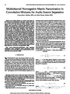
R Figure 1. The world of World of Warcraft . The figure shows a 2D projection of 150 million votes for guilds (green points) into the space spanned by the convex-hull NMF bases (red boxes). Intuitively understandable interpretations of the basis elements are written right next to them. Computing the factorization and the embedding took less than 1.5 hours on a standard desktop machine.
enforce W to represent meaningful “cluster centroids”. This is beneficial in many applications such as text and genome mining, as well as image and social network analysis. Although several (convex) NMF approaches have been proposed, very little work exists on how to apply NMF in the wild, i.e., with millions of data points. This is exactly the problem we examine in this paper. Our main contribution is convex-hull NMF, a very fast and scalable convex NMF technique. Triggered by the simple observation that each data point is a convex combination of vertices of the data convex hull, the key idea is to restrict W further to be vertices of the convex hull. The benefits are twofold: • First, the expected size of the convex hull typically grows slower than that of the data set. Consider for instance n random Gaussian points in the plane. Here the√expected number of vertices of the convex hull is Ω( log n). • Second, distance preserving low-dimensional embeddings allow one to compute candidate vertices efficiently. Our extensive experimental evaluation shows that convexhull NMF compares favorably to existing convex NMF methods for large data sets, both in terms of speed and reconstruction quality. Moreover, we show that convex-
hull NMF can be easily applied to large scale data sets. Specifically, we apply it to two large-scale, real world data sets, one consisting of 1.6 million images and one consisting R of 150 million votes on World of Warcraft guilds. We proceed as follows. We start of by reviewing NMF. Then, in Section III, we will develop convex-hull NMF. Section IV will present our experimental evaluation on several synthetic and real-world data sets. Before concluding, we will touch upon related work. II. N ON -N EGATIVE M ATRIX FACTORIZATION Assume an m × n input data matrix V = (v1 , . . . , vn ) consisting of n column vectors of dimensionality m. We consider factorizations of the form V ≈ Wm×k Hk×n . The resulting matrix W contains a set of k � n basis vectors which are linearly combined using the coefficients in H to represent the data. Common approaches to achieve such a factorization include Principal Component Analysis (PCA) [1], Singular Value Decomposition (SVD) [2], Vector Quantization (VQ), or non-negative Matrix Factorization (NMF) [3]. Note that the factorizations resulting from these methods differ since each method imposes other constraints: PCA constrains W to be composed of orthonormal vectors and results in a holistic H, VQ constrains H to unary vectors, and NMF assumes V, W and H to be non-negative matrices and often leads to part-based, sparse representations of the data. That is, in the case of NMF, the matrix W often represents meaningful parts and H tends to be sparse. From this point of view, NMF marks a middleground between distributed and unary representations [3]. In addition to the the data-compression aspects of NMF, the intuitive interpretability of the resulting factors makes it especially interesting for data-mining. Various variants and improvements to NMF have been introduced in recent year. For example, Cai et al. [4] present a matrix factorization that obeys the geometric data structue. In [5] a speed improvement to NMF is achieved using a novel algorithm based on an alternating nonnegative least squares framework. Another interesting variation is presented in [6] where optimization is based on a blockiterative acceleration technique. In this work, however, we build on Semi-NMF and Convex-NMF (C-NMF) recently introduced by Ding et. al [7]. Semi-NMF relaxes the nonnegativity constraint of NMF by allowing V and W to have mixed signs thereby extending the applicability of the method. Convex-NMF, on the other hand, represents the data matrix V as a convex combination of data points, i.e. V = VGHT
This is akin to Archetypal Analysis according to Cutler and Breiman [8] where both matrices G and HT are to be stochastic. Convex-NMF yields interesting interpretations of the data because each data point is now expressed as a weighted sum of certain data points. Consider e.g. Fig. 2. Here, we applied several NMF variants to analyze the CBCL Face Database 1 which consists of 2,429 19x19 gray-scale face images1 . As one can see, standard NMF results in part-based, sparse representations. Data points, however, do not correspond to convex combinations of these elementary parts. C-NMF, on the other hand, yields basis elements that allow for expressing data points as convex combinations of given data points. Accordingly, the “meaning” of these basis elements is intuitively understandable. In the following, we will briefly review C-NMF, its complexity and relevancy for data analysis. C-NMF as introduced in [7] minimizes J = kV − VGHT k2 , where V ∈ Rm×n , G ∈ Rn×k , H ∈ Rn×k . The matrices G and H are updated iteratively until convergence using the following update rules: s (Y+ H)ik + (Y− GHT H)ik Gik = Gik (1) (Y− H)ik + (Y+ GHT H)ik s (Y+ G)ik + (HGT Y− G)ik Hik = Hik (2) (Y− G)ik + (HGT Y+ G)ik where Y = VT V, and the matrices Y+ and Y− are given by 1 |Yik | + Yik 2 1 = |Yik | − Yik , 2
Yik+ = and Yik−
respectively. For the initialization of G and H two methods are proposed. The first initializes to (almost) unary representations based on a k-means clustering of V. The second assumes a given NMF or Semi-NMF solution. For further details on the algorithm and its initializations we refer to [7]. Note that, in our experimental evaluation in Section IV of this paper, we only present results where we initialized the methods in [7] using the first scheme since we did not find that the two alternatives yield significantly different reconstruction errors. Convex-NMF is related to k-means clustering and results in similar basis vectors W. However, it usually outperforms the k-means algorithm w.r.t. cluster accuracy. It is important to note that the C-NMF update rules in Eq. (1) and Eq. (2) have a time complexity of O(n2 ).
where each column i of G is a stochastic vector that obeys kgi k1 = 1, gi ≥ 0 .
1 MIT Center For Biological and Computation Learning, http://cbcl.mit. edu/projects/cbcl/software-datasets/
(a) Standard NMF
(b) Convex NMF
(c) Convex hull NMF
Figure 2. The basis vectors resulting from different NMF variants applied to the CBCL Face Database 1. (a) Standard NMF results in part-based, sparse representations. Data points cannot be expressed as convex combinations of these basis elements. (b) C-NMF yields basis elements that allow for convex combinations. Moreover, the basis vectors are “meaningful” since they closely resemble given data points. They are, however, not indicative of characteristic variations among individual samples. (c) CH-NMF as proposed in this paper results in non-negative factors that represent such variations in the data (e.g. pale faces, faces with glasses, faces with beards, etc.).
Moreover, although the iterative algorithm comes down to simple matrix multiplications, the size of the involved matrices quickly becomes another limiting factor (similar to the intermediate blowup problem in tensor decomposition [9]), since VT V results in an n×n matrix. Switching to an online update rule would avoid memory issues but it would at the same time introduce additional computational overhead. Overall, we can say that C-NMF does not scale to large data sets. In the following, we will present Convex-Hull NMF (CH-NMF), which is a novel C-NMF method for large-scale data analysis.
contrast to [7], we aim at factorizing the data such that each data point is expressed as a convex combination of convex combinations of specific data points. The task now is to minimize
2 J = V − VGHT (3)
III. C ONVEX -H ULL NMF
The intuition is as follows. Since we assume a convex combination for X, and by definition of the convex hull, the convex hull Hcvx (V) of V must contain X. Obviously, we could achieve a perfect reconstruction, giving J = 0, by setting G so that it would contain exactly one entry equal to 1 for each convex hull data point while all other entries were set to zero. Or more informal: following the definition of the convex hull we can perfectly reconstruct any data point by a convex combination of convex hull data points. Therefore, our goal becomes to solve Eq. (3) by finding k appropriate data points on the convex hull
2 J = V − XHT , (4)
Convex-Hull NMF aims at a data factorization based on the data points residing on the data convex hull. Such a data reconstruction has two interesting properties: first, the basis vectors are real data points and mark, unlike in most other clustering/factorization techniques, the most extreme and not the most common data points. Second, any data point can be expressed as a convex and meaningful combination of these basis vectors. This, however, offers interesting new opportunities for data interpretation, as indicated in Fig. 2 and further demonstrated in Section IV. Following Ding et al. [7], we consider a factorization of the form V = VGHT , where V ∈ Rm×n , G ∈ Rn×k , H ∈ Rn×k . We further restrict the columns of G and H to convexity, i.e., kgi k1 = 1, gi ≥ 0 khj k1 = 1, hj ≥ 0 . We note again that Ding et al. [7] also consider convex combinations but not for the matrix H. In other words, in
s.t.kgi k1 = 1, gi ≥ 0, khj k1 = 1, hj ≥ 0 . In the following, we set X = Vd×n Gn×k .
xi ∈ Hcvx (V), i = 1, . . . , k . This also explains why we termed our approach convex-hull NMF. However, finding a solution to Eq. (4) is not necessarily straight forward. Rather, it is known that the worst case complexity for computing the convex hull of n points in m m dimensions is Θ(n 2 ). Moreover, the number of convex hull data points may tend to n for high dimensional spaces,
Algorithm 1 Convex-hull NMF using eigenvector projection as a mechanism for subsampling the convex hull. 1: Compute k eigenvectors el , l = 1 . . . k of the covariance matrix of a data matrix Vm×n 2: Project V onto the 2D-subspaces T E2×n o,q = V [eo , eq ], o = 1 . . . k, q = 1 . . . k, o 6= q
3: 4:
Compute and mark convex hull data points Hcvx (Eo,q ) for each 2D projection Combine marked convex hull data points (using the original data dimensionality m) Sm×p = {Hcvx (E1,2 ), . . . , Hcvx (Ek−1,k )}
5:
Optimize
2 JS = S − SIp×k Jk×p s.t.kii k1 = 1, ii ≥ 0, kji k1 = 1, ji ≥ 0
6:
Optimize
2 J = vi − XhTi , i = 1 . . . n where X = Sm×p Ip×k , s.t.khi k1 = 1, hi ≥ 0
see e.g. [10], [11]. Consequently, computing the convex hull of large data-sets quickly becomes practically infeasible. In this paper, we therefore propose an approximate solution that subsamples the convex hull but still offers convenient data reconstruction. Our approach exploits the fact that any data point on the convex hull of a linear lower dimensional projection of the data also resides on the convex hull in the original data dimension. Formally, since V contains finitely many points and therefore forms a polytope in Rm , we can resort to the main theorem of polytope theory, see e.g. [12]. Theorem 1 (Main Theorem of Polytope Theory): Every image of a polytope P under an affine map π : x → Mx+t is a polytope. In particular, every vertex of an affine image of P , i.e., every point of the convex hull of the image of P , corresponds to a vertex of P . In other words, computing the convex hull of several 2D affine projections of the data offers a way of subsampling Hcvx (V). Moreover, this is an efficient way as computing the convex hull of a set of 2D points can be done in O(n log n) time, [13]. This subsampling strategy is the main idea underlying Convex-Hull NMF, and its soundness directly follows from Theorem 1. Moreover, various methods can be used for linearly projecting the data to a 2D space: (a) complete projections: for lower dimensional data it is possible to perform any pairwise projection of any data dimension. (b) random selection: randomly select the dimensions to be projected.
(c)
eigenvector projection: project the data using pairwise combinations of the first d eigenvectors of the covariance matrix of V. (d) fastmap: utilize fastmap projections [14]. For the experiments, we opted for eigenvector projections aiming for a data reconstruction of 95% by selecting the first l eigenvectors. The mean and covariance matrix of V are computed iteratively and the resulting matrices of size m×m and can be efficiently stored. However, for very large data sets and high dimensional spaces computing the covariance matrix can take some time, so that in these cases the fastmap initialization or random selection might be favorable. Choosing PCA for linearly projecting the data to a 2D space, i.e., following option (c) leads to the Convex-Hull NMF approach as summarized in Alg. 1. Here, triggered by the idea that the expected size of the √ convex hull of n Gaussian data points in the plane is Ω( log n) [15], we consider √ j linear 2D projections and extract approximately p = j log n point. This candidate set grows much slower than n. Give a candidate set of p convex hull data points S ∈ Hcvx (V), we now select those k convex hull data points that yield the best reconstruction of the remaining subset S. This, again, can be formulated as a convex NMF optimization problem and we now have to minimize the following reconstruction error
2 JS = Sm×p − Sm×p Ip×k Jk×p (5) under the convexity constraints kIi k1 = 1, Ii ≥ 0 kJi k1 = 1, Ji ≥ 0 .
Since p � n, solving (5) can be done efficiently using a quadratic programming solver. Note that the data dimensionality is m. The convex hull projection only served to determine a candidate set; all further computations are carried out in the original data space. By obtaining a sufficient reconstruction accuracy for S, we can set X = Sm×p Ip×k and thereby select k convex hull data points for solving Eq. (4). We found that I usually results in unary representations. If this is not the case, we simply map SI to their nearest neighboring data point in S. Given X, the computation of the coefficients H is straight forward. For smaller data-sets it is possible to use the iterative update rule from Eq. (2). However, since we do not further modify the basis vectors X, we can also find an optimal solution for each data point vi individually Ji = kvi − Xhi k2 using common solvers. Obviously, this can be easily parallelized.
Figure 4. Boxplots of reconstruction errors (in log-space) of k-means, CNMF, and CH-NMF for varying numbers of synthetically generated data. As one can see, CH-NMF outperforms both other methods significantly. (Best viewed in color.)
IV. E XPERIMENTAL E VALUATION In the following, we present experimental evaluation of CH-NMF on three data-sets. We decided for three experimental setups designed for evaluating different aspects of the proposed algorithm. Our first experimental setup evaluates and compares the run-time performance against C-NMF using synthetically generated data. As evaluation of C-NMF and other factorization methods for very large data-sets is often not feasible, we limit the maximum number of generated data to 4000 points. As we are mainly interested in the analysis of large real-world data sets, the last two experiments evaluate CH-NMF for two very large data-sets. Here, for evaluating the performance on high dimensional data, we decided for one rather low-dimensional and one high-dimensional data set. Thus, the first large data-set has only 80 dimensional feature vectors consisting of player activity scores for the Massively Multiplayer Online Game R (MMOG) World of Warcraft . The second consists of 1.6 million images of the Tiny image data-set [16]. The images are at size 32 × 32 resulting in 3072 dimensional feature vectors. Experimental evaluation is based on a basic Python implementation running on a standard IntelQuadcore 2.GHz computer. For optimization we used the cvxopt library by Dahl and Vandenberghe (http://abel.ee.ucla.edu/cvxopt/). Although CH-NMF can be easily parallelized, we used a strictly serial implementation. A. Synthetic Data Similar to the experimental procedure by Ding et al. [7], we evaluate the run-time performance using varying number of data points sampled from three randomly positioned
Figure 5. Boxplots of computation time (in log-space) for k-means, CNMF, and CH-NMF for varying numbers of synthetically generated data. It can be seen that for smaller data-set, up to 1000 samples, CH-NMF is actually significantly slower than C-NMF. However, for sample size larger than 1000 CH-NMF shows significant speed-ups. The computation time almost stays constant as it mainly grows with number of convex hull points and not with the size of the data. (Best viewed in color.)
Gaussians in 2D, see also Fig. 3. Besides measuring computation times, we also computed the mean reconstruction error. We compared CH-NMF against C-NMF and, as a baseline and because of its close connection to C-NMF, k-means clustering. We varied the number of sampled data points ranging from 100 to 4000 in steps of 100. To account for effects of random initializations we repeated each experiment 5 times. The number of basis vectors (or clusters for k-means) is set
Figure 3. Resulting basis vectors of convex-NMF, convex-hull-NMF, and NMF for data samples taken from three randomly placed Gaussian distributions in 2D. It can be seen that CH-NMF basis vectors reside on the convex hull of the data whereas C-NMF usually converges against cluster centroids. NMF basis vectors, in contrast, do not correspond to actual data points, however, they could be re-scaled to reside closer to actual data points. (Best viewed in color.)
to 6. The resulting average reconstruction errors can be seen in Fig. 4. The resulting runtime performance is shown in Fig. 5, both Figures have log space scaling. Following Ding et al. [7], we carried out 100 iterations for each approach. Overall CH-NMF leads to a very accurate data reconstruction. This follows the definition of the convex hull that is at the basis of our work. Using the convex-hull for reconstructing the inner data-points must lead to a perfect reconstruction. Since we exploit this property and subsample the convex hull we usually obtain very accurate data reconstruction. In comparison, C-NMF often converges against basis vectors that lie within data clusters. While this is by itself a wanted property, it leads to slightly worse reconstruction. A reason for this could be the non-negativity constraint of coefficients HT . This conic reconstruction limits perfect reconstruction to data-points within the conic hull of basis vectors [17]. Regarding runtime performance, it can be seen that while CH-NMF initially takes longer for fewer data-samples (up to 1000), its computation time increases moderately with an increase of data samples. This is explained √ by the moderate increase of convex hull data points Ω( log n) of a single Gaussian in the plane [15]. For k √ mixtures of Gaussians we usually have far less than Ω(k log n) convex hull data points. It also holds for larger number of samples, e.g. it takes about 54 seconds for 50000 data points. It should be noted that about 90% of the time is spent optimizing J =
vi − XhT 2 which could be done in parallel. Memory i requirements for CH-NMF are rather low as it requires to store l convex hull data points at maximum. B. World of Warcraft
R
This data-set consists of recordings of the online appearance of characters in the computer game World of R Warcraft . Since it is –to our knowledge– the first time that vast data recordings of Massively Multiplayer Online games are considered as a source for data mining, we will
briefly describe the data;it is assumed that World of World R of Warcraft has about 12 million p(l)aying customers. The game takes place in a virtual medieval fantasy environment. However, instead of one persistent world, players are distributed among different so called realms. These realms exist in parallel and can have slightly varying rule-sets, i.e. each realm is its own world. In the US and Europe there exist R about 500 unique realms. World of Warcraft is often considered one large social platform which is used for chatting, team-play, and gathering. Compared to well known virtual worlds that mainly serve as chat platforms such as, for R example, Second-life http://secondlife.com/, R
World of Warcraft is probably the real second life as it has a larger and more active (paying) user base. Moreover, a R whole industry is developing around World of Warcraft . It is estimated that 400.000 people world-wide are employed as gold-farmers, i.e. collecting virtual goods for online games and selling them over the Internet. Players organize in groups, which are guilds. Unlike groups known from other social platforms, such as Flickr, membership in a guild is exclusive. Obviously, the selection of a guild influences with whom players frequently interact. It also influences how successful players are in terms of game achievements, for instance how likely they are to obtain better equipment or rare items. The data was crawled from the publicly accessible site www.warcraftrealms.com. In the following, we interpret each character online appearance as a vote. Characters observations span a period of 4 years. Every time a character is seen online, he votes for the guild he is a member of according to his level. We accumulate the votes into a levelguild histogram, going from level 10 (level 1-9 are excluded) to level 80 (the highest possible level). Players advance in level by enganging in the game, i.e. completing quests or other heroic deeds. We assume that the level distribution among a guild is a good descriptor for its success. For example, a guild of
(a) improving, boost with 1st update (b) new formed guild of mostly high (c) formed after first update, boost (d) constant improve till 1st update no activity with 2nd update level players, disband after first up- with second update date
(e) high activity till 2nd update
(f) seldom active
(g) formed early then slowly disbanded after first update
(h) formed early then faded away
Figure 6. Basis vectors as the outcome of CH-NMF. Each subplot shows a level-guild histogram. The x-axis denotes histogram bins corresponding to player levels. Player levels describe a characters experience and can be increased over time. Each bin describes accumulated player votes in log-space. By definition of CH-NMF the basis vectors show the most extreme data-points. As CH-NMF yields meaningful basis vectors, one can easily provide intuitive descriptions of the basis vectors, as given in the subcaptions. For example, Subfig. 6(c) shows a guild that mainly consists of high level players ranging from level 70 to 80. Thus, we can assume that the guild was formed after the 2nd update when the level cap was raised to level 80, and then stayed together. Subfig. 6(h), as a second example, shows a high activity for lower levels up to level 30. Here, we can assume that the guild was formed early in the game and then disbanded.
very experienced level 80 characters has a higher chance for achievements than a guild of level 10 players. Also, a level histogram gives an indicator for player activity over time. If players are continuously staying with a particular guild, we expect an equally distributed level histogram, as the characters are continuously increasing their level over time. Following [18], we use logarithmic histogram values in our analysis. In total, we collected 150 million votes of 18 million characters belonging to 1.4 million guilds. R data Application of CH-NMF to the World of Warcraft revealed some very interesting structures. Fig. 7 shows a projection of all level-guild histograms into the space spanned by the CH-NMF basis vectors. We decided for 8 basis vectors since we assumed that one basis vector would function as a unity vector and encode a range of 10 levels. However, the actual outcome is quite different from what we expected, as can be seen in Fig. 6. Here it shows that the interpretability of basis vectors can be very useful for data-mining. By describing the basis vectors of CH-NMF that correspond to a particular guild, we gain an intuitively understandable distribution of all World of R Warcraft guilds. In particular, it is interesting that the majority of guilds is very close to the ”seldom active” guild. Thus, far more guilds or players seem to be casual gamers. In contrast, none of the most successful guilds belong to
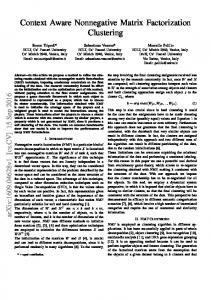
that group. Also, it is interesting to note that we can spot singular events, in our case large updates to the game content (this a regular procedure that makes novel content available and also allows a further advancement in character level), by looking at the level-guild histograms. Apparently, large updates to the game can result in a restructuring of social groups. Regarding runtime performance, the application of CHNMF took 57 minutes (this includes the complete algorithm described in Fig. 1). The computation of 8 basis vectors only took 7.5 minutes. As expected, most time was spent on computing the 1.4 million basis vector coefficients, and on the computation of level-guild histograms (about 20 minutes). C. Large-scale Image Collection The third data set we analyzed consists of 1.6 million images downloaded from the Internet [16]. The images are rescaled to 32 × 32 pixel, resulting in a 3072 dimensional feature vector. A projection of the data in the space spanned by 16 basis vectors can be seen in Fig. 8. Interestingly, some of the basis vectors found among the tiny images show a geometric similarity to Gabor filters that are found among the principal components of natural images [19]. This suggests that the extremal points in this large collection of natural images are located close to the principal axes of the
Figure 7. The world of World of Warcraft. We projected the guilds onto the space spanned by the 8 basis vectors as the outcome of CH-NMF. The guild names show locations of 13 of the 20 most successful guilds according to http://www.wowprogress.com/ (we do not yet have complete data, therefore we could not show the remaining 7). The right histogram next to each red marker shows the level-guild histogram corresponding to that basis vector. The left histogram shows how that basis vector is distributed among all guilds. As we have a convex combination of basis vectors, basis vector coefficients range between 0.0 and 1.0. We binned the coefficients into 10 bins per basis vector. Some of the histograms indicate power law distributions (histograms are plotted in log-space). The vast majority of guilds can be regarded as seldom active. Interestingly, the most successful guilds are clearly separated from the vast majority of guilds when represented using CH-NMF factorizations. (Best viewed in color.)
The Legacy EU-Mazrigos Closure EU-Stormscale Refuge EU-Aegwynn Risen EU-Illidan Wraith EU-Ysondre Security EU-Frostmane Ensidia EU-Magtheridon Apex EU-Al’Akir Premonition EU-Alleria For the Horde EU-Destromath Loot FTW EU-Twilight’s Hammer Method EU-Sylvanas Experience EU-Dentarg Last Resort EU-Kazzak Incorporated EU-Burning Steppes
6(a) 0.313 0.0 0.139 0.042 0.306 0.625 0.0 0.084 0.16 0.053 0.091 0.044 0.036 0.119 0.0
6(b) 0.185 0.4 0.373 0.144 0.0 0.021 0.0 0.0 0.013 0.0 0.0 0.0 0.318 0.499 0.237
Basis vector 6(c) 6(d) 0.33 0.119 0.325 0.0 0.455 0.0 0.454 0.001 0.31 0.23 0.146 0.08 0.552 0.0 0.634 0.072 0.545 0.0 0.396 0.2 0.428 0.169 0.485 0.412 0.555 0.0 0.202 0.007 0.417 0.0
coefficients 6(e) 6(f) 0.013 0.0 0.0 0.275 0.004 0.014 0.0 0.359 0.089 0.0 0.051 0.0 0.0 0.448 0.21 0.0 0.181 0.0 0.35 0.0 0.275 0.0 0.059 0.0 0.0 0.058 0.0 0.174 0.0 0.346
6(g) 0.04 0.0 0.0 0.0 0.065 0.077 0.0 0.0 0.102 0.0 0.038 0.0 0.007 0.0 0.0
6(h) 0.0 0.0 0.016 0.0 0.0 0.0 0.0 0.0 0.0 0.0 0.0 0.0 0.026 0.0 0.0
Table I R BASIS VECTOR COEFFICIENTS FOR A NUMBER OF SELECTED W ORLD OF WARCRAFT GUILDS ( CORRESPONDING BASIS VECTORS ARE EXPLAINED IN DETAIL IN F IG . 6). T HE GUILDS ARE SELECTED FROM A LIST OF THE TOP 20 WORLD WIDE GUILDS ACCORDING TO www.wowjutsu.com/world/. T HE COEFFICIENTS TEND TO BE SIMILAR HAVING E . G . A STRONG TENDENCY TOWARDS 6( C )) ”formed after first update, very active with second update” AS CAN ALSO BE SEEN IN THE PROJECTION IN F IG . 7.
data. Using larger numbers of basis vectors added more and more structured images to the set of basis images. Due to the high dimension of the data used application of R CH-NMF took longer than the World of Warcraft data. The reason is mainly the expensive computation of the covariance matrix required for the convex-hull projection. Here, the use of a faster projection scheme as proposed in Section III might be useful. Computing the covariance and the eigenvectors took about 1-2 days as we did not try to further optimize the process and simply iterated over all images. Application of CH-NMF took about 6 hours (approx. 3 hours for finding basis vectors and 3 hours for computing coefficients).
such as collaborative filtering. To improve performance, one could explore mixtures of convex hulls to deal with general distributions. Also, an analysis on how outliers effect the performance on small and medium size data sets should be done, as our results indicate that this is not an issue for very large data-sets. Finally, a comparison to max-margin matrix factorization [21], [22], which do a low-norm instead of a low-rank factorization, would be interesting. Overall our experimental results are an encouraging sign that applying NMF techniques in the wild, i.e., on millions of data points may not be insurmountable.
V. C ONCLUSIONS
The authors would like to thank A. Torralba, R. Fergus, and W. T. Freeman for making the tiny images freely available. Kristian Kersting was supported by the Fraunhofer ATTRACT Fellowship STREAM.
Machine learning and data mining techniques typically consists of two parts: the model and the data. Most effort in recent years has gone into the modeling part. Largescale datasets, however, allow one to move into the opposite direction [16], [20]: how much can the data itself help us to solve the problem. This direction is particularly appealing given that the Internet nowadays offers a plentiful supply of large-scale datasets for many challenging tasks. Motivated by this, we have presented a data-driven NMF approach, called convex-hull NMF, that is fast and scales well. The key idea is to restrict the ”clusters” to be combinations of vertices of the convex hull of the dataset; thus directly exploring the data itself to solve the convex NMF problem. Our experimental results reveal that convex-hull NMF can indeed effectively extract meaningful ”clusters” from datasets containing millions of images and rating. For future work it is interesting to apply convex-hull NMF to other challenging data-sets, such as Wikipedia, Netflix, Facebook, or the blogsphere, and to use it for applications,
Acknowledgements
R EFERENCES [1] I. Jolliffe, Principal Component Analysis.
Springer, 1986.
[2] G. Golub and J. van Loan, Matrix Computations, 3rd ed. Johns Hopkins University Press, 1996. [3] D. D. Lee and H. S. Seung, “Learning the parts of objects by non-negative matrix factorization,” Nature, vol. 401, no. 6755, pp. 788–799, 1999. [4] D. Cai, X. He, X. Wu, and J. Han, “Non-negative matrix factorization on manifold,” in International Conference on Data Mining. IEEE, 2008, pp. 63–72. [5] J. Kim and H. Park, “Toward faster nonnegative matrix factorization: A new algorithm and comparisons,” in International Conference on Data Mining. IEEE, 2008, pp. 353–362.
Figure 8. 1.6 million tiny images projected into the space spanned by 16 convex-hull NMF basis vectors. The displayed images show the basis vectors. Interestingly, the basis images often show plain colors, or a geometric similarity to Gabor filters. (Best viewed in color.)
[6] S. Suvrit, “Block-iterative algorithms for non-negative matrix approximation,” in International Conference on Data Mining. IEEE, 2008, pp. 1037–1042. [7] C. H. Ding, T. Li, and M. I. Jordan, “Convex and SemiNonnegative Matrix Factorizations,” IEEE Trans. on Pattern Analysis and Machine Intelligence, vol. 99, no. 1, 5555. [8] A. Cutler and L. Breiman, “Archetypal Analysis,” Technometrics, vol. 36, no. 4, pp. 338–347, 1994.
[16] A. Torralba, R. Fergus, and W. T. Freeman, “80 Million Tiny Images: A Large Data Set for Nonparametric Object and Scene Recognition,” IEEE Trans. on Pattern Analysis and Machine Intelligence, vol. 30, no. 11, pp. 1958–1970, 2008. [17] B. Klingenberg, J. Curry, and A. Dougherty, “”non-negative matrix factorization: Ill-posedness and a geometric algorithm”,” Pattern Recognition, vol. 42, no. 5, pp. 918 – 928, 2008.
[9] T. G. Kolda and J. Sun, “Scalable tensor decompositions for multi-aspect data mining,” in International Conference on Data Mining. IEEE, 2008, pp. 363–372.
[18] J. Aitchison, “The Statistical Analysis of Compositional Data,” J. of the Royal Statistical Society B, vol. 44, no. 2, pp. 139–177, 1982.
[10] D. Donoho and J. Tanner, “Neighborliness of RandomlyProjected Simplices in High Dimensions,” Proc. of the Nat. Academy of Sciences, vol. 102, no. 27, pp. 9452–9457, 2005.
[19] G. Heidemann, “The principal components of natural images revisited,” IEEE Transactions on Pattern Analysis and Machine Intelligence, vol. 28, no. 5, 2006.
[11] P. Hall, J. Marron, and A. Neeman, “Geometric Representation of High Dimension Low Sample Size Data,” J. of the Royal Statistical Society B, vol. 67, no. 3, pp. 427–444, 2005.
[20] A. Talwalkar, S. Kumar, and H. Rowley, “Large-scale manifold learning,” in Computer Vision and Pattern Recognition. IEEE, 2008.
[12] G. Ziegler, Lectures on Polytopes.
[21] N. Srebro, J. D. M. Rennie, and T. S. Jaakola, “Maximummargin matrix factorization,” in Advances in Neural Information Processing Systems 17. MIT Press, 2005.
Springer, 1995.
[13] M. de Berg, M. van Kreveld, M. Overmars, and O. Schwarzkopf, Computational Geometry. Springer, 2000. [14] C. Faloutsos and K.-I. Lin, “FastMap: A Fast Algorithm for Indexing, Data-mining and Visualization of Traditional and Multimedia Datasets,” in Proc. ACM SIGMOD, 1995. [15] I. Hueter, “Limit Theorems for the Convex Hull of Random Points in Higher Dimensions,” Trans. of the American Mathematical Society, vol. 351, no. 11, pp. 4337–4363, 1999.
[22] J. Rennie and N. Srebro, “Fast maximum margin matrix factorization for collaborative prediction,” in International Conference on Machine Learning, 2005.