Cross-Subject EEG Event-Related Potential Classification for Brain

Cross-Subject EEG Event-Related Potential Classification for Brain-Computer Interfaces Using Residual Networks Arnaldo Pereira, Dereck Padden, Jay Jantz, Kate Lin, Ramses Alcaide-Aguirre

To cite this version: Arnaldo Pereira, Dereck Padden, Jay Jantz, Kate Lin, Ramses Alcaide-Aguirre. Cross-Subject EEG Event-Related Potential Classification for Brain-Computer Interfaces Using Residual Networks. 2018.

HAL Id: hal-01878227 https://hal.archives-ouvertes.fr/hal-01878227 Submitted on 20 Sep 2018

HAL is a multi-disciplinary open access L’archive ouverte pluridisciplinaire HAL, est archive for the deposit and dissemination of sci- destinée au dépôt et à la diffusion de documents entific research documents, whether they are pub- scientifiques de niveau recherche, publiés ou non, lished or not. The documents may come from émanant des établissements d’enseignement et de teaching and research institutions in France or recherche français ou étrangers, des laboratoires abroad, or from public or private research centers. publics ou privés. Copyright

Cross-Subject EEG Event-Related Potential Classification for Brain-Computer Interfaces Using Residual Networks Arnaldo E. Pereira Neurable, Boston, MA

Dereck Padden Neurable, Boston, MA

[email protected]

[email protected]

Jay J. Jantz Centre for Neuroscience Studies, Queen’s University Kingston, Ontario [email protected]

Kate Lin Wellesley College Wellesley, MA

Ramses E. Alcaide-Aguirre Neurable, Boston, MA [email protected]

Abstract EEG event-related potentials, and the P300 signal in particular, are promising modalities for brain-computer interfaces (BCI). But the nonstationarity of EEG signals and their differences across individuals have made it difficult to implement classifiers that can determine user intent without having to be retrained or calibrated for each new user and sometimes even each session. This is a major impediment to the development of consumer BCI. Recently, the EEG BCI literature has begun to apply convolutional neural networks (CNNs) for classification, but experiments have largely been limited to training and testing on single subjects. In this paper, we report a study in which EEG data were recorded from 66 subjects in a visual oddball task in virtual reality. Using wide residual networks (WideResNets), we obtain state-of-the-art performance on a test set composed of data from all 66 subjects together. Additionally, a minimal preprocessing stream to convert EEG data into square images for CNN input while adding regularization is presented and shown to be viable. This study also provides some guidance on network architecture parameters based on experiments with different models. Our results show that it may possible with enough data to train a classifier for EEG-based BCIs that can generalize across individuals without the need for individual training or calibration.

1. Introduction A brain-computer interface (BCI) is a device that allows a user to interact with a computer through neural activity

[20, 7]. BCIs were originally conceived as a way to allow paralyzed individuals to communicate [11] and move around [1]. And while that is still a primary motivation behind BCI research, the last decade has seen an increased interest in the potential uses of BCIs—EEG-based BCIs, in particular—for hands-free interaction with consumer devices, industrial applications, and entertainment [37, 1, 2]. BCIs may even be a viable interaction method for virtual reality and augmented reality applications [37, 22]. One of the most-commonly studied signals in EEGbased BCIs is the P300 event-related potential (ERP) [29]. The P300 is so called because it is characterized by a positive peak approximately 300ms after the subject attends to an “oddball” target stimulus among several similar but nontarget stimuli [11]. The stimuli can be visual, such as flashing rows and columns of letters [11, 7, 38], objects, faces, or scenery [32, 28], or geometric shapes [8]. But they can also be auditory [5] or tactile [23]. The common denominator is the “oddball” task design. Despite recent progress in the BCI literature, there are a few major obstacles preventing the widespread deployment and adoption of EEG-based BCIs. First, noninvasive methods such as EEG have a low signal-to-noise ratio [29, 36]. Second, the EEG signals that are used to determine user intent in these applications—such as the P300— are highly specific to each person and can even vary significantly within an individual over time [47, 35]. While the first problem can be addressed with more or less success through signal filtering [36, 3, 6], the second problem has been harder to deal with. In practice, that difference in signal profiles across people and data sessions has meant that most classifiers used to detect EEG event-related potentials

in real time are trained specifically for each user and often even for a particular data session [29]. The solution to this problem is to find a way to train EEG classifiers that can generalize across people and time. Convolutional neural networks have recently gained attention in the EEG literature [7, 32, 28, 38, 26] because of their feature-extraction properties [6] and success in image classification [34]. We extend this line of work by applying wide residual networks (WideResNets) [46] with spatial dropout [40, 43] and cutout [10] to 6-electrode EEG data obtained from 66 subjects performing a visual oddball task in virtual reality. This paper presents a minimal preprocessing stream to convert EEG epochs into images. We then examine the performance of ResNets [15, 16] of different widths and depths on ERP detection. Furthermore, we study the effect of using cutout for regularization of EEG data. Our experiments show that convolutional networks can classify target vs nontarget stimuli accurately on a test set taken from many subjects, and that it may be possible with enough data to train a classifier that can detect ERPs in the general population without any need to calibrate or train specifically for an individual user at runtime.

2. Motivation and Related Work Convolutional neural networks (CNNs) are excellent at classifying images of objects belonging to different classes [25, 39, 42, 41]. In a convolutional network, lower-level representations of the image are convolved with a learned kernel to extract higher-level features from a larger region of the image [48, 34, 25]. Multiple convolutional layers can be stacked to extract progressively higher-level feature maps [48, 34]. CNNs have gained attention in recent years as a possible solution for EEG signal classification because of their power to extract nonlinear and holistic features from their input data. The first study to use convolutional neural networks to classify P300s was done by Cecotti and Gr¨aser [7]. The input to their network for each epoch of data to be classified is a tensor of dimensions Nelectrodes × Nsamples . Their network was composed of the input layer just described, feeding into a first hidden spatial convolution layer of NF M feature maps with a convolution kernel of size (Nelectrodes × 1), then a second convolutional layer producing NF M × 5 feature maps, which performs time convolution and downsampling with a kernel of length 13 = Nsamples , followed by a fully connected layer and an ouput 3 layer of two neurons representing the probabilities of the two classes (target and nontarget). Similar studies followed. The authors of [6] used a simplified version of the Cecotti-Gr¨aser network to explore the spatial filters learned by the first convolutional layer and compared the results to those obtained by using xDAWN [36] and CSP spatial filters [3]. Manor and Geva added a

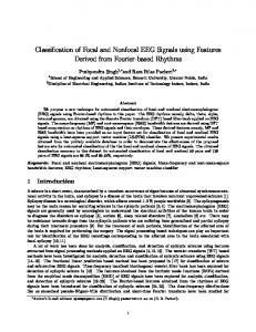
Figure 1: Visual stimuli presented during the EEG recording task. Subjects were instructed to make a mental note when the object indicated by a white circle flashed and to ignore the flashing of all other objects.

max-pooling layer [27] after the intial spatial convolution and replaced the single temporal convolution and downsampling layer of the Cecotti-Gr¨aser network with temporal convolution → max pooling → temporal convolution. They also incorporated ReLU [33] and dropout [40] into their network. The network in [28] was also based on the Cecotti-Gr¨aser architecture, but it added batch normalization [21] after the input and temporal convolution layers. As in Manor and Geva [32], Liu et al. used ReLU activations in their convolutional layers. Other studies used networks with similar network architectures [38, 26]. A few P300 studies using convolutional neural networks have experimented with input tensors different from the ones in Cecotti and Gr¨aser [5, 31, 23]. The paper of Kodama and Makino [23] is the closest to our approach to network input. The authors of that study created a 20 × 20 square matrix from the time series data for each electrode and then then joined the feature matrices from each of 8 electrodes, plus one feature matrix created from the average of all 8 electrodes, into a single 2D input tensor for each epoch of EEG data [23]. Our method also represents an entire EEG data epoch as a single 2D tensor, but we arrange our data in a way that we believe better preserves its temporal information in the deeper layers of the network and adds regularization

3. Materials and Methods 3.1. EEG Dataset Sixty-six subjects participated in a visual oddball task in virtual reality. Each subject wore a Neurable DK1 headset (Neurable, Inc., Boston, Mass.), which comprises an HTC Vive (HTC, New Taipei City, Taiwan) virtual reality headset

equipped with DSI dry EEG electrodes (Wearable Sensing, San Diego, Cal.) at the P4, Pz, P3, PO8, PO7, and Oz locations. EEG was sampled at 300Hz. The experiment was programmed in the Unity game engine (Unity Technologies, San Francisco, Cal.) using the Neurable SDK, which allows synchronization of stimuli presented in virtual reality using Unity with the EEG data from the electrodes attached to the headset. A screenshot from the experiment is presented in Figure 1. The subjects were placed in a room in virtual reality while seated on chair to maintain an approximately fixed distance to a plane presenting five toy objects: a ring stack, a train, a ball, a cube, and an airplane. Each recording session consisted of 10 trials. In each trial, one of the five objects was randomly selected as the target by having a solid white circle appear around the item. This solid circle stayed around the item for the duration of the trial. Subjects were instructed to make a mental note when the target object for the current trial flashed and to ignore the flashing of the remaining four objects. Each trial comprised 10 sequences. A sequence consisted of each of the five objects flashing bright green once in a random order. That is, in a given trial the first sequence could consist of the flash order airplane, ball, cube, ring stack, train, while the second sequence might be ball, ring stack, train, cube, airplane, and the third might be train, airplane, cube, ring stack, ball, and so on for the given number of sequences per trial. Each flashing object was highlighted in bright green for 60ms. Within a trial, the interstimulus time in between the end of one flash and the beginning of the next one was 100ms. There was a pause of approximately 3s in between trials. During this pause the circle around the target object disappeared and the subject was shown an animation of the object floating towards the subject. The object would then return to its original position along the other four objects and a new circle would appear around another object, indicating it as the target for the next trial. For each stimulus, an EEG data epoch was extracted consisting of the 800ms of recorded data for all 6 electrodes beginning with the stimulus flash onset. Thus, there were 10 × 10 × 5 = 500 labeled EEG epochs for each session: 100 target epochs and 400 nontarget epochs. Additionally, 3 of the sessions (1 session each from subjects 1, 4, and 25) were mistakenly recorded at 6 sequences per trial rather than 10 sequences per trial. Seeing no downside other than the loss of the extra data which could have been acquired in those sessions, we opted to keep those 3 sessions in the dataset. There were a total of 233 data sessions recorded (across all subjects). In total the dataset consists of 115900 EEG epochs. To create a training and test set, the target and nontarget epochs in each session were separated. The targets and nontargets were then separately shuffled and 80% of each designated for training,

Figure 2: Visualization of a random subset of 50 target epochs (red crosses) and 50 nontarget epochs (blue stars) using t-SNE [30].

with the other 20% set apart for testing. The training sets from all sessions were then combined and shuffled to form a single large cross-subject and cross-session train set, and the same was done to create a combined test set. The final distribution of the data is shown in Table 1. As seen in Figure 2, the classes are not separable by a simple surface even in the high-dimensional space of the original features.

Train Test

Target 18480 4620

Nontarget 73920 18480

Table 1: Description of dataset. EEG epochs from each session were split 80%/20% between training and test sets and combined into a single cross-subject and cross-session training set and test set.

3.2. Data Preprocessing This section describes our method for turning each raw EEG data epoch into a 2D image-like input tensor. For convenience, we abbreviate Nelectrodes as Ne and Nsamples as Ns . Each raw epoch data matrix E has a shape Ne × Ns . Ns in the case of the data above is 240, since the epochs are each 800ms and the data is sampled at Fs = 300Hz. A characteristic P300 signal is expected around 300ms after stimulus onset in the target epochs but not in the nontarget epochs [11, 7]. Additionally, there might be an attentional [12] or visual component of the event-related potential around 100ms after onset that correlates with the target/nontarget label [4, 17]. Figure 3 shows a P300 epoch and an NP300 epoch in their time series and image forms. We apply the minimal preprocessing described below to each epoch to turn it from raw temporal data into an input

cording to eq. (2). We choose this method rather than the block layout of [23] because in Kodama’s method corresponding time samples taken from highly correlated electrodes can be in distant parts of the image, limiting the effectiveness of regularization methods like cutout. 0 D1,1

 (a)

(b)

DSq

  D 0 √M  1, Ne +1 = ..   .  0 D (√M −1)√M 1,

(c)

(d)

Figure 3: Examples of EEG epoch data as electrode timeseries data and as images. (a): A single target epoch after bandpass filtering and decimation. (b): A single nontarget epoch after bandpass filtering and decimation. Note the possible P300 peak around 380ms in the target epoch and a negative peak around 120ms (a possible N100 related to attending to a nontarget stimulus [12]) in the nontarget epoch. (c), (d): The same epochs as images after preprocessing. image for the CNN. Minimal data processing is emphasized for two reasons. First, in online applications the data preprocessing must not be too computationally expensive. Second, we are using CNNs precisely for their power as feature extractors. Each epoch E is bandpass filtered to 2–9Hz. The signal data is then decimated by a factor of 2. We then find an amount of padding P for the decimated matrix D of dimensions Ne × Nd such that: For Ne , Nd , P 0 ∈ Z+ , p M ≡ Ne (Nd + 2P 0 ) P = argmin{M | M ∈ Z+ }

(1)

P0

Each electrode time series is padded with P zeros at either end. Let Di,t indicate the tth time sample taken from electrode i. There are Nd = 120 samples per electrode after decimation and our Ne = 6. Therefore, we pad each Di with P = 15 zeros at the beginning and at the end, ending up with a padded D0 of dimensions M = 6 × 150 = 900, with Np = 150 samples for each electrode after padding. D0 is then reshaped into a 30 × 30 square matrix DSq ac-

Ne

0 D2,1

D0

√ 2, NM e

... +1

...

D0

√

..

+1

. ...



Ne , NM e D0 2√M Ne , Ne 0 DN e ,Np

      

(2) Then, the entries di,j of DSq are discretized into 256 bins and normalized to be in [0, 1]. We preprocess the data this way for two reasons. First, CNN architectures have been designed for and tested most extensively on square, discrete image data of this form. Therefore, heuristics and parameters developed for classifying image data will likely transfer most readily to data in this form. Second, by discretizing the data into 256 bins we reduce the entropy of our input layer Hin . Therefore, discretizing the input data shrinks the search space for future weight vectors. In particular, let Hc1 be the entropy of the output tensor from the convolutional layer connected to the input layer. Hc1 = F(Hin , pc1 ), where F is a increasing function in Hin and pc1 , and pc1 is a constant that depends on the input dimensions and the convolution kernel size, stride, and number of output feature maps. And likewise, for a second convolution following the first Hc2 = F(F(Hi n, pc1 ), pc2 ) is also increasing in Hin , and so on. Intuitively, the space of feature maps that a convolutional layer can produce given all possible discretized inputs is smaller than the space of all feature maps it could produce given all possible nondiscretized inputs from the same distribution. Therefore, this discretization acts as a regularizer.

3.3. Neural Network Architectures A ResNet [15, 16] is a CNN that uses residual units that add the output of convolutional layers and activations to the input to the residual unit by using skip connections. Several variations of residual convolutional networks (ResNets), introduced in [15] and refined in [16], are currently the state of the art [18, 45, 14, 13, 10] in image classification on the CIFAR [24] and ImageNet [9] datasets. Following [16, 46, 10], our networks use preactivation. That is, batch normalization and dropout precede the convolutional layers in the residual blocks. We use the term residual block to refer to the structure shown in Figure 4b, which in turn is composed of one or more stacked residual units. A residual unit takes the form: Y = C ◦ R ◦ B ◦ · · · ◦ C ◦ R ◦ B ◦ C(X) + P(X)

(3)

(a)

(b)

Figure 4: The networks studied in this paper follow the WideResNet architecture templates from [46]. For convolutional layers, FM , [x, y] indicates convolutions in that layer or block output FM feature maps and use a kernel of size [x, y]. (a): The generic WideResNet architecture. The number of output feature maps for each residual block is given in parentheses. The global average pooling layer is densely connected to a two-way softmax at the top. (b): The architecture of the bth residual block of the network with width parameter k and depth parameter n. All convolutions use a stride of [1, 1], except the first convolutions of residual blocks 2 and 3, which use a stride of [2, 2] for downsampling. A curved arrow indicates a skip connection. Arch.

Params

Cutout

Acc.

Bal. Acc.

Precision

Recall

False Alarm

WRN– 16–1

175K

Yes

73.87%

64.03%

39.83%

58.82%

WRN– 16–2

700K

No Yes

72.92% 77.06%

62.66% 64.96%

37.78% 43.35%

WRN– 16–4

2.75M

No Yes

77.75% 79.34%

65.10% 67.15%

11M

No Yes

78.58% 80.51%

No

80.06%

WRN– 16–8

F1

22.35%

False Omission 11.77%

0.4750

55.82% 47.66%

22.84% 15.62%

12.45% 13.43%

0.4506 0.4540

44.20% 48.15%

43.75% 43.15%

13.77% 11.61%

13.99% 13.85%

0.4397 0.4551

65.88% 68.82%

45.90% 51.63%

41.93% 41.23%

12.30% 9.67%

14.15% 14.00%

0.4383 0.4585

68.03%

50.23%

40.60%

10.06%

14.18%

0.4490

Table 2: Architectures with depth fixed at d = 16 weight layers, with and without cutout. (Mean of 5 bootstrapped runs on random 80% subsets of the test data.) The best results for each metric are shown in bold. In eq. (3), B means batch normalization, R represents ReLU activation, and C means convolution. X and Y are the input and output tensors, respectively. P is a projection

such that the right- and left-hand sides of the addition have the same dimensions. P can be the identity or a [1, 1] convolution with stride [2, 2] for downsampling—the two op-

Arch.

Params

Cutout

Acc.

Bal. Acc.

Precision

Recall

False Alarm

F1

11.79%

False Omission 13.79%

CNN– 10–8 WRN– 10–8 WRN– 16–8 WRN– 22–8 WRN– 28–8 WRN– 40–8

4.6M

Yes

79.25%

66.86%

47.51%

43.09%

4.8M

Yes

79.56%

66.97%

48.94%

37.12%

9.77%

14.91%

0.4222

11M

Yes

80.51%

68.82%

51.63%

41.23%

9.67%

14.00%

0.4585

17M

Yes

79.47%

67.46%

48.74%

43.53%

11.50%

13.82%

0.4599

23M

Yes

74.52%

64.09%

40.19%

56.73%

21.04%

12.02%

0.4705

36M

Yes

78.95%

66.51%

47.11%

42.22%

11.86%

14.09%

0.4453

0.4519

Table 3: Architectures with width parameter fixed at k = 8. (Mean of 5 bootstrapped runs on random 80% subsets of the test data.) The best results for each metric are shown in bold. F1

Trained on

Tested on

9.67%

False Omission 14.00%

0.4585

66

66

58.82%

22.35%

11.77%

0.4750

66

66

40.9%

69.2%

20.02%

7.14%

0.5141

1

1

– 70.0% 67.56%

– – 42.14%

70% 64.4% 69.47%

19.11% 23.7% 19.07%

– – 7.02%

– – 0.5246

1 1 1

1 1 1

57.35%

18.39%

97.40%*

86.46%*

3.70%

0.3094

9

1

Model

Acc.

Bal. Acc.

Precision

Recall

False Alarm

WRN– 16–8 WRN– 16–1 Cecotti & Gr¨aser Manor & Geva Speller Objects Liu et al. Kodama & Makino Corrected for 5 : 1 class priors

80.51%

68.82%

51.63%

41.23%

73.87%

64.03%

39.83%

78.19%

66.87%

79.1% 75.0% 79.02%

27.52%

Table 4: Model comparison. We use the best reported results on target/nontarget classification tasks run on fewer than 3 subjects. For tasks with more than 3 subjects where the authors reported mean metrics, we present those. Where a metric was not reported in a paper but it could be calculated from the reported results, we have calculated it. The best results for each metric are shown in bold. tions we use, following the findings in [46]. But it can also be some other mapping of the input X into the same space as the left-hand side of the sum. We use residual units of length 2 for all our networks, again following the results of [46] and [10]. Different WideResNet [46] architectures were tested on

our data, with and without cutout [10]. The name of each network tested describes its architecture. So, for example, WRN–16–2 indicates a network with a depth of 16 weight layers and a width parameter k = 2. A width parameter k = 1 corresponds to the architecture template of [16]. The depth d of the network is an integer d satisfying d = 6n + 4,

1 TP 1 TN + 2 TP + FP 2 TN + FN TP Precision = TP + FP TP Recall = TP + FN FP False Alarm = TN + FP FN False Omission = TN + FN Precision−1 + Recall−1 −1 ) F1 = ( 2 Bal Acc. =

(a)

(b)

(c)

(d)

Figure 5: (a)–(d): Cutout of 15 × 15 randomly applied four times to the same epoch. for n ∈ Z+ , n > 0. All networks use in this paper follow the architecture pattern shown in Figure 4. Training parameters generally followed those for the CIFAR datasets in [46] and [10].The loss function was crossentropy weighted to account for the 4 : 1 class inbalance between target and nontarget stimuli. Dropout of 0.3 was used between convolutional layers in the residual blocks. The models trained with cutout use a 15 × 15 cutout square. See Figure 5 for an example of how cutout was applied to our data. No data augmentation was used.

4. Results All models were programmed in Keras with a TensorFlow back end and trained on an NVIDIA Tesla V100 GPU. In Table 2 we show the results of runs with networks of depth d = 16 and width parameter k = 1, 2, 4, 8, with and without cutout. The effect of depth on performance was tested by fixing the width at k = 8 and changing the depth to 10, 22, 28, and 40 weight layers. For the experiments with varying depth we used cutout on all models. Those results are shown in Table 3. We report the following metrics, with T P , T N , F P , and F N standing for true positives, true negatives, false positives, and false negatives, respectively: Acc. =

TP + TN TP + FP + TN + FN

(4)

(5) (6) (7) (8) (9) (10)

It is important to break down performance in this way because of the class imbalance inherent in oddball tasks. For example, for tasks with a 5 : 1 class imbalance, which is common in the literature, a classifier could obtain a raw accuracy value of 83.33% simply by predicting nontarget for every epoch given to it. Table 4 compares our best model and our smallest model to other convolutional neural network models from the literature. Manor and Geva reported performance metrics on two oddball tasks: a 6 × 6 speller and a task where the subjects where presented photographs belonging to different categories. We show their performance on each of those tasks.

5. Discussion Our top model (WRN–16–8) outperforms the top CNN models in the P300 BCI literature for which metrics broken down by target/nontarget class are available or could be calculated on accuracy, precision, and false-alarm rate. The same model also comes in a close second in terms of balanced accuracy. And, as shown in Table 4, even our smallest model (WRN–16–1)—which has only 175K parameters— performs competitively with the current state-of-the-art results for CNN EEG classifiers. But whereas—with the exception of Kodama and Makino—the results in the literature have been obtained by training a model or an ensemble of models on data from a single human subject and testing on that same single subject, we demonstrate that is possible to train CNN models that can learn generalizable features from the EEG data of many subjects and still classify accurately between target and nontarget stimuli. On our EEG data, added regularization from cutout generally improves results, as shown in Table 2. The only exception out of the networks tested was WRN–16–2, and even there the gain in recall and accuracy was obtained at the expense of precision. The model of [23] has the highest recall and, consequently, also the lowest false omission rate by far. But that is a result of the model predictions being biased towards the target class, which is undesirable in a practical BCI. For practical consumer BCIs precision is more important than recall, since it is always possible to

flash another sequence to obtain confirmation of the user’s intent. That is no doubt inconvenient—but less so than having the device take unintended actions. As expected given the empirical findings on ImageNet and CIFAR in [46] and [44], depth is not the primary driver of accuracy. While the initial proposition for why ResNets work was that the skip connections allow more gradient to flow back through the network during the backpropagation step of training, thus allowing CNNs to grow deeper and deeper while still being able to converge [15, 16], empirical work in [46] showed that shallower but wider networks— i.e., shallower networks with more feature maps in the intermediate layers—could outperform deeper networks with the same computational budget. One interpretation of why this happens is the fact that a ResNets with s skip connections can be conceptualized as ensemble of 2s networks [44, 19]. Empirically, most of the gradient of deep ResNets tends to flow through shorter rather than longer paths [44]. This is one possible explanation for why the deeper networks in Table 3 do not outperform shallower networks. Depth helps up to a point, because depth is created by adding residual units and, therefore, expanding the number of paths through the network. After a certain point, however, additional longer paths may not account for much of the backpropagation gradient [44], but the added parameters may result in overfitting. This observation is consistent with [46] and our own observations on EEG data. In terms of EEG data, our models are essentially ensembles of smaller networks looking at the EEG data at different levels of spatiotemporal resolution. Because successive convolutional layers have larger and larger receptive fields for each of their neurons, adding skip connections allows shorter paths to examine the EEG data at a finer resolution, while longer paths are looking at the EEG epoch at a more holistic level. Therefore, a residual network should be expected to outperform a CNN with the same architecture (minus the skip connections). To test this hypothesis we compared a ResNet and a CNN of the same depth in Table 3, and indeed we find that this is true for our data. Even the shallowest ResNet that can be built with the architecture in Figure 4 outperforms an equivalent network with the skip connections taken out.

6. Conclusion We show that ResNet models can accurately classify EEG epochs from many subjects into target and nontarget classes based on user intent. The models demonstrated in this paper perform better than the best CNN models in the EEG literature in terms of accuracy, precision, and falsealarm rate—even though those models are trained and tested on an individual subject and the models presented here train and test on 66 different subjects together. Additionally, this study shows the viability of a minimal preprocessing stream

to transform EEG data into an input compatible with CNN models traditionally used for image classification, while at the same time adding regularization. Cutout is shown to be effective for regularizing EEG data transformed into images. Finally, our work offers a theoretical explanation for why ResNets can perform so well on EEG epochs. The main takeaway from this study is that ResNets trained on a large and representative cross-section of the population may be viable models for consumer brain-computer interfaces that do not require a calibration or training phase for each new user.

References [1] A. Barachant, S. Bonnet, M. Congedo, and C. Jutten. Multiclass braincomputer interface classification by Riemannian geometry. IEEE Transactions on Biomedical Engineering, 59(4):920–928, 2012. [2] A. Barachant and M. Congedo. A plug&play P300 BCI using information geometry. CoRR, abs/1409.0107, 2014. [3] B. Blankertz, R. Tomioka, S. Lemm, M. Kawanabe, and K. Muller. Optimizing spatial filters for robust EEG singletrial analysis. IEEE Signal Processing Magazine, 25(1):41– 56, 2008. [4] G. Bonmassar, D. P. Schwartz, A. K. Liu, K. K. Kwong, A. M. Dale, and J. W. Belliveau. Spatiotemporal brain imaging of visual-evoked activity using interleaved eeg and fmri recordings. Neuroimage, 13(6):1035–1043, 2001. [5] E. Carabez, M. Sugi, I. Nambu, and Y. Wada. Convolutional neural networks with 3D input for P300 identification in auditory brain-computer interfaces. Computational Intelligence and Neuroscience, 2017:8163949, 2017. [6] H. Cecotti, M. P. Eckstein, and B. Giesbrecht. Single-trial classification of event-related potentials in rapid serial visual presentation tasks using supervised spatial filtering. IEEE Transactions on Neural Networks and Learning Systems, 25(11):2030–2042, 2014. [7] H. Cecotti and A. Gr¨aser. Convolutional neural networks for P300 detection with application to brain-computer interfaces. IEEE Transactions on Pattern Analysis and Machine Intelligence, 33(3):433–445, 2011. [8] R. Das, E. Maiorana, and P. Campisi. Visually evoked potential for eeg biometrics using convolutional neural network. In 2017 25th European Signal Processing Conference (EUSIPCO), pages 951–955, 2017. [9] J. Deng, W. Dong, R. Socher, L.-J. Li, K. Li, and L. Fei-Fei. ImageNet: A Large-Scale Hierarchical Image Database. In CVPR09, 2009. [10] T. Devries and G. W. Taylor. Improved regularization of convolutional neural networks with cutout. CoRR, abs/1708.04552, 2017. [11] L. A. Farwell and E. Donchin. Talking off the top of your head: A mental prosthesis utilizing event-related brain potentials. Electroencephalography and Clinical Neurophysiology, 70(6):510–523, 01 1988. [12] L. Garc´ıa-Larrea, A.-C. Lukaszewicz, and F. Maugui´ere. Revisiting the oddball paradigm. non-target vs neutral stimuli

[13] [14]

[15]

[16] [17]

[18] [19]

[20]

[21]

[22]

[23]

[24] [25]

[26]

[27]

and the evaluation of ERP attentional effects. Neuropsychologia, 30(8):723–741, 1992. X. Gastaldi. Shake-shake regularization. CoRR, abs/1705.07485, 2017. D. Han, J. Kim, and J. Kim. Deep pyramidal residual networks. 2017 IEEE Conference on Computer Vision and Pattern Recognition (CVPR), pages 6307–6315, 2017. K. He, X. Zhang, S. Ren, and J. Sun. Deep residual learning for image recognition. In 2016 IEEE Conference on Computer Vision and Pattern Recognition (CVPR), pages 770– 778, 2016. K. He, X. Zhang, S. Ren, and J. Sun. Identity mappings in deep residual networks. CoRR, abs/1603.05027, 2016. M. J. Herrmann, A.-C. Ehlis, H. Ellgring, and A. J. Fallgatter. Early stages (P100) of face perception in humans as measured with event-related potentials (erps). Journal of neural transmission, 112(8):1073–1081, 2005. G. Huang, Z. Liu, and K. Q. Weinberger. Densely connected convolutional networks. CoRR, abs/1608.06993, 2016. G. Huang, Y. Sun, Z. Liu, D. Sedra, and K. Q. Weinberger. Deep networks with stochastic depth. In B. Leibe, J. Matas, N. Sebe, and M. Welling, editors, Computer Vision – ECCV 2016, pages 646–661, Cham, 2016. Springer International Publishing. J. E. Huggins, R. E. Alcaide-Aguirre, and K. Hill. Effects of text generation on P300 brain-computer interface performance. Brain-Computer Interfaces, 3(2):112–120, 2016. S. Ioffe and C. Szegedy. Batch normalization: Accelerating deep network training by reducing internal covariate shift. In F. Bach and D. Blei, editors, Proceedings of the 32nd International Conference on Machine Learning, volume 37 of Proceedings of Machine Learning Research, pages 448–456, Lille, France, 07–09 Jul 2015. PMLR. J. J. Jantz, A. Molnar, and R. Alcaide. A braincomputer interface for extended reality interfaces. In Proceedings of SIGGRAPH ’17 VR Village, 2017. https://doi.org/10.1145/3089269.3089290. T. Kodama and S. Makino. Convolutional neural network architecture and input volume matrix design for erp classifications in a tactile p300-based brain-computer interface. In 2017 39th Annual International Conference of the IEEE Engineering in Medicine and Biology Society (EMBC), pages 3814–3817, 2017. A. Krizhevsky, V. Nair, and G. Hinton. Cifar-10 (canadian institute for advanced research). A. Krizhevsky, I. Sutskever, and G. E. Hinton. Imagenet classification with deep convolutional neural networks. In Proceedings of the 25th International Conference on Neural Information Processing Systems - Volume 1, NIPS’12, pages 1097–1105, 2012. V. J. Lawhern, A. J. Solon, N. R. Waytowich, S. M. Gordon, C. P. Hung, and B. J. Lance. Eegnet: a compact convolutional neural network for eeg-based braincomputer interfaces. Journal of Neural Engineering, 15(5):056013, 2018. Y. LeCun, K. Kavukcuoglu, and C. Farabet. Convolutional networks and applications in vision. In Proceedings of 2010 IEEE International Symposium on Circuits and Systems, pages 253–256, 2010.

[28] M. Liu, W. Wu, Z. Gu, Z. Yu, F. Qi, and Y. Li. Deep learning based on batch normalization for P300 signal detection. Neurocomputing, 275:288–297, 2018. [29] F. Lotte, L. Bougrain, A. Cichocki, M. Clerc, M. Congedo, A. Rakotomamonjy, and F. Yger. A review of classification algorithms for EEG-based brain-computer interfaces: A 10year update. Journal of Neural Engineering, 15(3):031005, 2018. [30] L. v. d. Maaten and G. Hinton. Visualizing data using t-SNE. Journal of machine learning research, 9(Nov):2579–2605, 2008. [31] R. K. Maddula, J. T. Stivers, M. Mousavi, S. Ravindran, and V. R. de Sa. Deep recurrent convolutional neural networks for classifying P300 BCI signals. 2017. [32] R. Manor and A. B. Geva. Convolutional neural network for multi-category rapid serial visual presentation BCI. Frontiers in Computational Neuroscience, 9:146, 2015. [33] V. Nair and G. E. Hinton. Rectified linear units improve restricted boltzmann machines. In Proceedings of the 27th International Conference on International Conference on Machine Learning, ICML’10, pages 807–814, 2010. [34] W. Rawat and Z. Wang. Deep convolutional neural networks for image classification: A comprehensive review. Neural Computation, 29(9):2352–2449, 2017. [35] B. Reuderink, J. Farquhar, M. Poel, and A. Nijholt. A subject-independent brain-computer interface based on smoothed, second-order baselining. In 2011 Annual International Conference of the IEEE Engineering in Medicine and Biology Society, pages 4600–4604. IEEE, 2011. [36] B. Rivet, A. Souloumiac, V. Attina, and G. Gibert. xDAWN algorithm to enhance evoked potentials: Application to braincomputer interface. IEEE Transactions on Biomedical Engineering, 56(8):2035–2043, 2009. [37] R. Scherer, M. Chung, J. Lyon, W. Cheung, and R. P. Rao. Interaction with virtual and augmented reality environments using non-invasive brain-computer interfacing. In 1st International Conference on Applied Bionics and Biomechanics (October 2010), 2010. [38] H. Shan, Y. Liu, and T. Stefanov. A simple convolutional neural network for accurate P300 detection and character spelling in brain computer interface. In Proceedings of the Twenty-Seventh International Joint Conference on Artificial Intelligence, IJCAI-18, pages 1604–1610. International Joint Conferences on Artificial Intelligence Organization, 7 2018. [39] K. Simonyan and A. Zisserman. Very deep convolutional networks for large-scale image recognition. 09 2014. [40] N. Srivastava, G. Hinton, A. Krizhevsky, I. Sutskever, and R. Salakhutdinov. Dropout: A simple way to prevent neural networks from overfitting. Journal of Machine Learning Research, 15:1929–1958, 2014. [41] C. Szegedy, S. Ioffe, V. Vanhoucke, and A. A. Alemi. Inception-v4, inception-resnet and the impact of residual connections on learning. In AAAI, volume 4, page 12, 2017. [42] C. Szegedy, W. Liu, Y. Jia, P. Sermanet, S. Reed, D. Anguelov, D. Erhan, V. Vanhoucke, and A. Rabinovich. Going deeper with convolutions. In 2015 IEEE Conference on Computer Vision and Pattern Recognition (CVPR), 2015.

[43] J. Tompson, R. Goroshin, A. Jain, Y. LeCun, and C. Bregler. Efficient object localization using convolutional networks. 2015 IEEE Conference on Computer Vision and Pattern Recognition (CVPR), pages 648–656, 2015. [44] A. Veit, M. Wilber, and S. Belongie. Residual networks behave like ensembles of relatively shallow networks. pages 550–558, 2016. [45] S. Xie, R. Girshick, P. Doll´ar, Z. Tu, and K. He. Aggregated residual transformations for deep neural networks. In Computer Vision and Pattern Recognition (CVPR), 2017 IEEE Conference on, pages 5987–5995. IEEE, 2017. [46] S. Zagoruyko and N. Komodakis. Wide residual networks. CoRR, abs/1605.07146, 2016. [47] P. Zanini, M. Congedo, C. Jutten, S. Said, and Y. Berthoumieu. Transfer learning: A riemannian geometry framework with applications to braincomputer interfaces. IEEE Transactions on Biomedical Engineering, 65(5):1107– 1116, 2018. [48] M. D. Zeiler and R. Fergus. Visualizing and understanding convolutional networks. In D. Fleet, T. Pajdla, B. Schiele, and T. Tuytelaars, editors, Computer Vision – ECCV 2014, 2014.