Current approaches to gene regulatory network modelling

BMC Bioinformatics

BioMed Central

Open Access

Review

Current approaches to gene regulatory network modelling Thomas Schlitt1 and Alvis Brazma*2 Address: 1Department of Medical and Molecular Genetics, King's College London School of Medicine, 8th floor Guy's Tower, London SE1 9RT, UK and 2European Bioinformatics Institute, EMBL-EBI, Wellcome Trust Genome Campus, Cambridge CB10 1SD, UK Email: Thomas Schlitt - [email protected]; Alvis Brazma* - [email protected] * Corresponding author

Published: 27 September 2007
Otto Warburg International Summer School and Workshop on Networks and Regulation
Peter F Arndt and Martin Vingron Reviews

BMC Bioinformatics 2007, 8(Suppl 6):S9

doi:10.1186/1471-2105-8-S6-S9

This article is available from: http://www.biomedcentral.com/1471-2105/8/S6/S9 © 2007 Schlitt and Brazma; licensee BioMed Central Ltd. This is an open access article distributed under the terms of the Creative Commons Attribution License (http://creativecommons.org/licenses/by/2.0), which permits unrestricted use, distribution, and reproduction in any medium, provided the original work is properly cited.

Abstract Many different approaches have been developed to model and simulate gene regulatory networks. We proposed the following categories for gene regulatory network models: network parts lists, network topology models, network control logic models, and dynamic models. Here we will describe some examples for each of these categories. We will study the topology of gene regulatory networks in yeast in more detail, comparing a direct network derived from transcription factor binding data and an indirect network derived from genome-wide expression data in mutants. Regarding the network dynamics we briefly describe discrete and continuous approaches to network modelling, then describe a hybrid model called Finite State Linear Model and demonstrate that some simple network dynamics can be simulated in this model.

Introduction Most cellular processes involve many different molecules. The metabolism of a cell consists of many interlinked reactions. Products of one reaction will be educts of the next, thus forming the metabolic network. Similarly, signalling molecules are interlinked and cross-talk between the different signalling cascades forms the signalling network. And the same is true for regulatory relationships between genes and their products. All these networks are closely related, e.g. the regulatory network is influenced by extracellular signals. But there are characteristic features in the signalling network, which do not exist in the regulatory network; therefore dealing with these networks separately makes sense. Our main interest is in transcription regulation networks and we will refer to them as "gene networks", but many principles are valid for a wide range of networks. High-throughput technologies allow studying aspects of gene regulatory networks on a genome-wide scale and we will discuss recent advances as well as limitations and future challenges for gene network

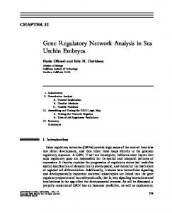
modelling. This survey is largely based on and is an extension of two previous publications [1,2]. Gene networks are concerned with the control of transcription, i.e. how genes are up and down regulated in response to signals. In the 1960's genetic and biochemical experiments demonstrated the presence of regulatory sequences in the proximity of genes and the existence of proteins that are able to bind to those elements and to control the activity of genes by either activation or repression of transcription. These regulatory proteins are themselves encoded by genes (Figure 1). This allows the formation of complex regulatory networks, including positive and negative feedback loops. These principles of gene regulation apply to prokaryotes (e.g. bacteria) as well as to eukaryotes (e.g. higher organisms). The control of gene activity is much more complex than Figure 1 suggests. It involves many kinds of proteins thus allowing additional levels of control particularly in eukaryotes. Transcription factors, the proteins that recognize the regulatory ele-

Page 1 of 22 (page number not for citation purposes)


ments in the DNA (the binding sites) need to interact with other proteins in order to activate gene expression. In addition to control of gene expression there are regulatory controls to determine the maturation, transport and degradation of the mRNA, as well as its translation. Just to illustrate the complexity of gene regulation: Gene Ontology (GO), a controlled vocabulary used to describe protein functions contains currently over 7500 different terms describing biological process 'transcription', including over 6500 terms under process 'regulation of transcription' [3]. Gene networks are often described verbally in combination with figures to illustrate sometimes-complicated interrelations between network elements. Due to the complexity of these networks, such models are not always easy to comprehend and they often leave a considerable amount to ambiguity to the reader's imagination. Since the 1960's methods from mathematics and physics have been used to describe and simulate small gene networks more stringently. Nowadays, molecular biological methods and high-throughput technologies make it possible to study a large number of genes and proteins in parallel enabling the study of larger gene networks. This allows tackling gene networks more efficiently and has led to a new discipline called Systems Biology, which seeks to combine methods from biology with methods from mathematics, physics and engineering to describe biological systems. We proposed to categorize gene networks models in four classes according to increasing level of detail in the models [1]. Each class has its own advantages and limitations. The four classes are: i. parts lists – a collection, description and systematisation of network elements in a particular organism or a particular biological system (e.g., transcription factors, promoters, and transcription factor binding sites); ii. topology models – a description of the connections between the parts; this can be viewed as wiring diagrams where directed or undirected connections between genes represent different types of interactions; iii. control logic models – a description of combinatorial (synergetic or interfering) effects of regulatory signals – e.g., which transcription factor combinations activate and which repress the transcription of the gene; iv. dynamic models – the simulation of the real-time behaviour of the network and the prediction of its response to various environmental changes, external, or internal stimuli.

http://www.biomedcentral.com/1471-2105/8/S6/S9

Obviously, for a fixed number of network elements each next level is more detailed and complex. But the size of the networks that we are able to model at each particular level is limited. Much larger networks can be described on topological level than on the dynamic level. In the following section we will discuss these classes in more detail.

Organisational levels of gene network models "All models are wrong, but some are useful". – George E. P. Box Parts list Compiling the parts list is the first step in developing any model of some complexity and is not always a trivial exercise. Simple parts lists of genes, transcription factors, promoters, binding sites and other molecular entities are useful means for assessing the network complexity and for comparing different organisms. Such parts lists can be the result of a genome-sequencing and annotation project, where the complete DNA sequence of an organism is determined and all (or at least many) genes and proteins are identified. A parts list could also be represented as a database of regulatory elements or it could be ontology terms of transcription regulation processes assigned to a set of genes.

Comparing such lists from different organisms can provide an indication of the complexity of the transcriptional machinery or be used to predict the presence or absence of particular metabolic pathways [4-6]. The number of known and predicted transcriptional regulators in eukaryotic organisms varies from about 300 in yeast to about 1000 in humans (Table 1). Many publications address the computational identification of transcription factor binding sites for instance by analysing promoter sequences of coexpressed genes [7]. One approach is to search for short sequences that are overrepresented in the promoters of a particular group of genes (e.g. clusters of coexpressed genes or sets of longer sequences known to bind a particular transcription factor) in comparison to the promoter sequences of all other genes. This approach obviously depends on the availability of the sequences for many genes and their upstream regions. Such an approach was applied in a cell cycle study in Schizosaccharomyces pombe, where Rustici et al. showed that the presence or absence of consensus binding sites in the promoter regions corresponds to the cyclic expression pattern of the genes [8]. Genes with a peak expression at similar cell cycle stage often share similar sets of consensus binding sites. However, the exact promoter regions are usually unknown and even the transcription start sites are only known for a few genes. Baker's yeast (Saccharomoyces cerevisiae) has a relatively small genome with short intergenic



GENE 1

GENE 2

GENE 3

http://www.biomedcentral.com/1471-2105/8/S6/S9

GENE 4

DNA

transcription factor binding site in promoter region coding DNA transcription factor

work 1 Representation Figure of a simple, fictional transcription factor netRepresentation of a simple, fictional transcription factor network. All genes shown encode transcription factors that control the activity of genes encoding transcription factors.

regions, considering about 600–1000 bp upstream of the translation start site (ATG) appears to be a good approximation for the promoter regions. In higher organisms like vertebrates the intergenic regions and thus the putative promoter regions are much larger than in yeast, therefore the identification of regulatory elements in the DNA sequence by computational means has turned out to be rather elusive. Some studies have focused on the computational analysis of higher-level organisation of transcription factor binding sites in promoters, such as frequently occurring combinations of known binding sites [9,10], or restricted the search for regulatory elements to conserved sequence regions, identified by genome comparisons, a method often referred to as phylogenetic footprinting [11]. However, phylogenetic footprinting does not always work, because the localisation and the binding sites themselves are not always conserved [12,13]. Transcription factor localisations can be identified experimentally, too. For example, individual binding sites can be detected using the "DNAse I footprinting assay"; proteins bound to the DNA protect it from degradation by DNAse I, therefore these regions can be analysed further [14]. Another common experimental method is the "electrophoretic mobility shift assay" (EMSA) sometimes called "band shift assay" or "gel retardation assay" – DNA

fragments that are bound by protein move slower in an electrophoretic gel than unbound fragments [15,16]. These methods allow fine mapping of individual binding sites, but are very labour intensive. High-throughput methods such as the Chip-on-chip method (see additional file 2, which describes this methods in more detail) allow the genome-wide detection of binding sites for a transcription factor, but the spatial resolution and signal quality is limited. Furthermore, assigning transcription factors to their target genes based on the genomic localisation is difficult due to the size of intragenic and intronic regions and long range effects of some transcription factors. Nevertheless parts lists provide the first impression of gene networks in different organisms and they are necessary to have before we continue by having a look at the network topology. Topology models Once we know the transcription factors and their binding sites, we can describe the gene transcription regulatory networks by graphs with nodes corresponding to genes and edges to regulatory interactions [17]. (Note the difference between these discrete graphs and plots of mathematical functions also often referred to as graphs.) A short introduction to discrete graphs is given in additional file 1, for more details please consult for example Cormen et al. [18]. One important concept that we will use below is a representation of a graph by a so-called adjacency matrix, where the element aij in a row i and column j equals 1 (i.e., aij = 1), if node i is connected to node j, otherwise aij = 0. Graph representations have been used for various biological data sets ranging from protein-protein interactions networks to coexpression networks, they have been long used in mathematics, physics and computer science, and many aspects of graphs and their applications have been studied (e.g., [19-21]).

In a directed graph (i.e., a graph where connections between nodes have a definite direction) we call genes (nodes) with outgoing edges (arcs) source genes. For a given source gene, we call the set of all genes with incoming arcs from that source gene its target genes. Regulatory relationships can be of various natures. For a specific

Table 1: Number of transcription regulators in different organisms

Organism yeast fly human

number of genes

number of transcription regulators

6682 13525 22287

312 (4.7%) 492 (3.6%) 1034 (4.6%)

The number of genes and transcriptional regulators (genes annotated with GO term GO:0030528 "transcription regulator activity" for yeast (Saccharomyces cerevisiae) was taken from SGD http://db.yeastgenome.org/cgi-bin/SGD/search/featureSearch and for fly (Drosophila melanogaster, DROM3) and human (Homo sapiens, NCBI 34 dbSNP120) was taken from ENSEMBL http://www.ensembl.org/Multi/martview



model we need to define the precise meaning that we assign to the edges (Figure 2). For instance, an arc from a gene A to B may mean that source gene A is a transcription factor, which is known to bind to the promoter of target gene B. A rather different network will be obtained if an arc from A to B denotes the observation that the disruption (e.g., mutation) of source gene A changes the expression of target gene B. We will present examples for these types of networks in the next section. A widely studied type of molecular network of a different type is the protein-protein interaction network, where the nodes represent proteins and two proteins are connected by an undirected edge, if they bind to each other (Figure 2) [22]. A different network will be established by connecting genes based on their sequence similarity. Networks can also be built based on the co-occurrence of gene names in journal abstracts. If two gene names frequently occur in the same abstracts it is likely that they share some kind of functional relationship [23]. To illustrate knowledge that we can obtain from studying network topology, we will compare and combine information from two high throughput data sets for the yeast Saccharomyces cerevisiae. The first is obtained from chromatin immunoprecipitation experiments for transcription factors (ChIP network), while the second is obtained from microarray experiments on single gene deletion mutants (mutant network), for more detail on the experimental methods please refer to additional file 2. Microarray experiment measurements can be presented in a data matrix, where rows represent genes and columns particular experiments (hybridisations). For instance, in the ChIP experiment each column will correspond to a particular transcription factor (studied in the particular experiment), while in the mutant experiment each column will correspond to a particular mutant. In this way, not only rows, but also columns will correspond to genes. The measurement values are typically real numbers, such as intensity levels, expression levels, or p-values, depending on the data processing steps applied. By applying an additional data processing step, often called thresholding, we can transform these continuous values into discrete values (e.g., if we chose a threshold t, then we can replace any xij by 0, if xij 2 no D=1

C>3 yes

D=0

where gi(t + Δt) is the expression level of gene i at time t + Δt, and wij the weight indicating how much the level of gene i is influenced by gene j (i,j = 1...n). Note that this model assumes a linear logic control model – the expression levels of genes at a time t+Δt, depends linearly on the expression levels of all genes at a time t. For each gene, one can add extra terms indicating the influence of additional substances [64].

B

A>5 no

gn(t+Δt) - gn(t) = (wn1 g1(t) + ... + wnn gn(t)) Δt

no

yes

E=1

E=0

if A>5 and B5 and B>2 then D=0 if A