Data Mining Challenges in Automated Prompting Systems Barnan Das Washington State University Pullman WA 99164
[email protected] (208) 596-1169
Diane J. Cook Washington State University Pullman WA 99164
[email protected] (509) 335-4985
ABSTRACT
classifiers is to predict if a particular step of an activity needs a prompt or not. Therefore, we can view automated prompting as a binary class learning problem. However, PUCK should deliver a prompt only when it is critically important rather than at every possible step, which would make PUCK a cause of annoyance rather than an aid. Intuitively, there are far more "no-prompt" instances in the dataset than "prompt" because there are very few situations that would require a prompt, thus making the data in this domain inherently skewed or in other words causing the class imbalance problem.
With the rising cost of medical treatment and majority of the aging population preferring an independent lifestyle, the need for assistive technologies and smarted devices are increasing like never before. A prompting system is a technique that provides interventions to a smart home inhabitant in order to ensure successful completion of an activity. Machine learning techniques could be used to automate this system but it comes with the challenge of imbalanced class distribution naturally occurring in the data. In this paper, we comparatively analyze two techniques (sampling and cost sensitive learning) to deal with this challenge.
In this work, we comparatively analyze the techniques that deal with imbalanced class distribution in the domain of automated prompting. Unlike other domains of class imbalance, automated prompting has a number of requirements that need to be taken care of. The focus is mainly on two different techniques: Sampling and Cost Sensitive Learning, to resolve the issue. In Sampling we introduce a version of SMOTE, developed by Chawla et al [2], called SMOTE-Variant. This version of SMOTE addresses the domain data challenges. We also consider Cost Sensitive Learning in which we empirically find the cost matrix that would be suitable for our work.
Author Keywords
Automated prompting, smart environments, data mining. ACM Classification Keywords
H5.m. Information interfaces and presentation (e.g., HCI): Miscellaneous. INTRODUCTION
Prompts in the context of a smart home environment can be defined as any form of verbal or non-verbal intervention delivered to a user on the basis of time, context or acquired intelligence that helps in successful (in terms of time and purpose) completion of an activity. Prompts can provide critical service in a smart home setting especially to older adults and inhabitants with some form of cognitive impairment. In our previous work [1], we have developed an automated prompting system, named Prompting Users and Control Kiosk or PUCK that predicts when a user would need a prompt while performing an activity. Thus, although not a “single” smart device, PUCK is an effective smart framework. Developing automated prompting systems like PUCK requires a unique combination of pervasive computing and machine learning techniques. One of the major challenges that need to be addressed to optimize performance of such systems is learning from imbalanced class distributions. The purpose of the
RELATED WORK
Prompting systems have been in existence for quite some time with different research groups offering their own unique approach to solving the problem. The approaches can be broadly classified into four types: Rule based (time and context), Reinforcement Learning, Planning and Supervised Learning. The majority of reminder systems are rule based. In this approach, a set of rules is defined based on time, context of doing an activity and user preferences. Lim et al. [3] proposed a medication reminder system that recognizes the reminders suitable for medication situation. Rudary et al. [4] integrated temporal constraint reasoning with reinforcement learning to build an adaptive reminder system. Although this approach is useful when there is no direct or indirect user feedback, it relies on a complete schedule of user activities. The Autominder System [5] developed by Pollack et al. provides adaptive personalized reminders of activities of daily living using a dynamic Bayesian network as an underlying domain model to coordinate preplanned events. Boger et al. [6] designed a Markov decision process (MDP) based planning system to determine when and how to provide prompts to dementia
Permission to make digital or hard copies of all or part of this work for personal or classroom use is granted without fee provided that copies are not made or distributed for profit or commercial advantage and that copies bear this notice and the full citation on the first page. To copy otherwise, or republish, to post on servers or to redistribute to lists, requires prior specific permission and/or a fee.
1
patients for guidance through the activity of hand washing. A supervised learning approach can help in fully automating the determination of a prompt situation using a set of features that would be characteristic of “prompt” or “no-prompt” situations. However, very limited work has been in this area. SYSTEM ARCHITECTURE
PUCK is not just a single device but a framework that helps in providing smart interventions to inhabitants of a smart home environment. The system architecture of PUCK in Figure 1 can be broadly divided into four major modules: Smart Environment: This is the smart home infrastructure that acts as a testbed where experiments are performed. It has a sensor network that keeps track of the activities performed and stores the data in a SQL database in real time. Data Preparation: Raw sensor data is collected from the database, manually annotated and features, that would be helpful in differentiating a “Prompt” step from a “No-Prompt” step, are generated. Because there are very few training examples that have “Prompt” steps, we use a sub-module, namely Sampling, to generate new and unique “Prompt” examples (more discussion later). Machine Learning Model: Once the data is prepared by the Data Preparation Module, we employ machine learning strategies to identify whether a prompt should be issued. This module is the “brain” of the entire system where the decision making process takes place. Prompting Device: This device acts as a bridge between the user or inhabitant and the digital world of sensor network, data and learning models. Prompting devices can range from simple speakers to basic computers, PDAs, or even smart phones (a project that we are planning to pursue in the near future).
time. In the past we have deployed rule based and context aware prompts at the homes of two participant older adults. In these deployments we used touch screen monitors with embedded speakers to deliver the prompts. The prompts included audio cues along with images that are relevant to the activity for which the prompt is being given. We are in the process of using this same interface for the automated prompting system. The following sections give a better understanding of the PUCK emphasizing more on the process model and thus implicitly covering the detailed description of the modules. EXPERIMENTAL SETUP Smart Home Testbed
The data collection is done in collaboration with the Department of Psychology at Washington State University. The smart home testbed is a 2 story apartment located on the WSU campus. It contains a living room, dining area and kitchen on the first floor and three bedrooms and bathroom on the second. All of these rooms are equipped with a grid of motion sensors on the ceiling, door sensors on the apartment entries and on cabinets, the refrigerator and the microwave oven, temperature sensors in each room, a power meter, and analog sensors for burner and water usage.
Figure 2. Three-bedroom smart apartment used for data collection (Sensors: motion (M), temperature (T), water (W), burner (B), telephone (P) and item (I)).
Figure 1. System Architecture of the PUCK.
In our current work we have been able to reach the phase where the system is able to predict a relative time in the activity when a prompt is required, after learning intensively from training data collected over a period of
Figure 1 depicts the structural and sensor layout of the apartment. Data was collected while volunteer older adult participants performed activities in the smart apartment. One of the bedrooms on the second floor is used as a control room where the experimenters monitor the activities performed by the participants (via web cameras) and deliver pre-defined prompts through an audio delivery system whenever necessary. The goal of PUCK is to learn from this collected data how to time the delivery of prompts and ultimately to automate the role of the experimenter in this setting. The following activities are used in our experiments: Sweep, Refill Medication, Birthday Card, Watch DVD, Water Plants, Make Phone Call, Cook and Select Outfit. These activities are subdivided into relevant steps by the
Feature Generation
psychologists in order to track their proper completion. Here is an example of the Cooking task.
From the annotated data we generate relevant features that would be helpful in predicting whether a step is a “Prompt” step or a “No Prompt” step. After the features are generated, the modified form of the data set contains steps performed by participants as instances. This data set is then re-annotated for the prompt steps. Table 2 provides a summary of all generated features.
Cooking 1. Participant retrieves materials from cupboard. 2. Participant fills measuring cup with water. 3. Participant boils water in microwave. 4. Participant pours water into cup of noodles. 5. Participant retrieves pitcher of water from refrigerator. 6. Participant pours glass of water. 7. Participant returns pitcher of water. 8. Participant waits for water to simmer in cup of water. 9. Participant brings all items to dining rooms table.
TABLE 2. List of Features and Description Feature # Feature Name
Participants are asked to perform these specific activities in the smart apartment. While going through the steps of an activity, a prompt is given if he/she performs steps for other activities rather than the current one, if a step is skipped, if extra/erroneous steps are performed, or if too much time has elapsed since the beginning of the activity. Note that there is no ideal order of steps by which the activity can be completed. Therefore, a prompt is given only when one of the conditions mentioned above occurs. Moreover, the goal is to deliver as few prompts as possible. The experimenters keep track of all the errors done by the participants and the steps at which a prompt was delivered, which are later extracted and used to train PUCK. Data Preparation Annotation
stepLength
Length of the step in time (seconds)
2
numSensors
Number of unique sensors involved with the step
3
numEvents
Number of sensor events associated with the step
4
prevStep
Previous step
5
nextStep
Next step
6
timeActBegin Time (seconds) since beginning of the activity
7
timePrevStep
8
stepsActBegin Number of steps since beginning of the activity
9
activityID
10
stepID
11
M01 … M51
12
Class
Time (seconds) between the end of the previous step and the beginning of the current step
Activity ID Step ID Frequency of firing each sensor during the step Binary Class. 1=”Prompt”, 0=”No Prompt”
We use data collected from 128 older adult participants, with different levels of mild cognitive impairment (MCI), to train the learning models. Thus the errors committed by the participants are real and not simulated. There are 53 steps in total for all the activities, out of which 38 are recognizable by the annotators. The participants were delivered prompts in 149 cases which involved any of the 38 recognizable steps. Therefore, approximately 3.74% of the total instances are positive (“Prompt” steps) and the rest are negative (“No-Prompt” steps). Essentially, this means that, predicting all the instances as negative, would give more than 96% accuracy even though all the predictions for positive instances were incorrect.
Table 1. Sample of sensor events used for our study
2009-05-11 2009-05-11 2009-05-11 2009-05-11 2009-05-11 2009-05-11 2009-05-11 2009-05-11 2009-05-11
1
DATASET AND PERFORMANCE METRIC
An in-house sensor network captures all sensor events and stores them in a SQL database in real time. The sensor data gathered for our SQL database is expressed by several features, summarized in Table 1. These four fields (Date, Time, Sensor, ID and Message) are generated by the data collection system. Date 2009-02-06 2009-02-06 2009-02-06 2009-02-05 2009-02-09
Description
Time 17:17:36 17:17:40 11:13:26 11:18:37 21:15:28
14:59:54.934979 14:59:55.213769 15:00:02.062455 15:00:17.348279 15:00:34.006763 15:00:35.487639 15:00:43.028589 15:00:43.091891 15:00:45.008148
Sensor ID M45 M45 T004 P001 P001 D010 M017 M017 M017 M018 M051 M016 M015 M014
Message ON OFF 21.5 747W 1.929kWh CLOSE ON OFF ON ON ON ON ON ON
The conventional performance measures (accuracy and error rate) consider different classification errors as equally important. However, this assumption is not realistic in the automated prompting domain where false positives are more acceptable than false negatives. Therefore, we consider performance metrics that measure the classification performance on positive and negative classes independently. True Positive (TP) Rate: represents the percentage of activity steps that are correctly classified as requiring a prompt; True Negative (TN) Rate: represents the percentage of correct steps that are accurately labeled as not requiring a prompt; Area Under ROC Curve (AUC): evaluate overall classifier performance without taking into account class distribution or error cost; Geometric mean of
7.3 7.4 7.8 7.8 7.8 7.8 7.9 7.9
Figure 3. Annotation with Steps
After collecting data, sensor events are labeled with the specific activity and step within the activity, {activity#.step#}, that was being performed while the sensor events were generated, as shown in Figure 3.
TP Rate and TN Rate (Gacc): given by
3
TPRate Rate ;
reflects the overall effects of classification on the data; and Accuracy (Acc): conventional accuracy of classifiers.
TP Rate
TN Rate
AUC
Gacc
Accuracy
J48
0.141
0.994
0.615
0.3744
96.21
value of k is small, we would have null neighbors. Due to these limitations we make variations that would suit our domain. Unlike SMOTE, we do not find the k nearest neighbors for all instances in the minority class. An instance is randomly picked from the minority class. All minority class instances that have the same activityID and stepID are considered as its nearest neighbor of the chosen instance. One of these neighbors is randomly chosen and the new instance is synthesized as done in SMOTE. Undersampling is done by randomly choosing a sample of size k (as per the desired size of the majority class) from the entire population without repetition. Here is the pseudo code for our approach:
SMO
0.013
0.999
0.506
0.1140
96.23
Algorithm: SMOTE-Variant (T, N, M)
LB
0.040
0.999
0.865
0.1999
96.36
EXPERIMENTAL EVALUATIONS
We conduct experiments to evaluate the machine learning approaches that we used in PUCK: decision tree (J48), support vector machines (SMO) and boosting (LogitBoost). All of the experiments are evaluated with 10 fold cross validation. Table 3 summarizes the overall performance. Table 3. Performance of Classifiers on Original Dataset
As mentioned before, classical machine learning approaches are not capable of handling this degree of skew. The inductive bias of a decision tree prefers shorter hypothesis trees over longer ones and thus compromises the unique properties of the instances that might lie with an attribute that has not been considered. In case of SMO, with 61 attributes in our case, it constructs a set of hyperplanes for classification. Usually a good separation is achieved by a hyperplane that achieves the largest distance to the nearest training data points of any class (the functional margin). However, due to the lesser number of positive class instances in our case the functional margin is quite small causing a lower TP rate. In our Boosting technique, a learning algorithm is run several times, each time with a different subset of training examples. Dietterich demonstrated [7] that this technique works well for algorithms whose output classifier undergoes major changes in response to small changes in the training data, also known as unstable learning algorithms. As a decision tree is an unstable algorithm, we use Decision Stump, a decision tree with the root node immediately connected to the terminal nodes, as the base learner. Sampling
Sampling is a technique of rebalancing the dataset synthetically. However, under-sampling can throw away potentially useful data, oversampling can overfit the classifier if it is done by data replication [8]. As a solution SMOTE [2] uses a combination of both under and over sampling, but without data replication. Over-sampling is performed by taking each minority class sample and synthesizing a new sample by randomly choosing any or all (depending upon the desired size of the class) of its k minority class nearest neighbors. Generation of the synthetic sample is accomplished by first computing the difference between the feature vector (sample) under consideration and its nearest neighbor. Next, this difference is multiplied by a random number between 0 and 1. Finally, the product is added to the feature vector under consideration. In our dataset the minority class instances are not only small in terms of percentage of the entire dataset, but also in absolute number. Therefore, if the nearest neighbors are conventionally calculated (as in original SMOTE) and the
Input: All the instances of minority class stored in list T, Number of minority class samples N, Desired number of minority class samples M Output: M minority class samples stored in list S if (M > N) then S = T //S stores all the instances in T for i ← 1 to M – N t = randomize(T) //Randomly chosen instance from T neighbor[] = null //List storing all the nearest neighbors of instance t for j ← 1 to length(T) if (t.activityID==T[j].activityID) AND (t.stepID==T[j].stepID) neighbor[].append(T[j]) // Appending the list with the neighbor endfor s = randomize(neighbor) //Randomly choosing an instance from list neighbor diff = t – s //Both t and s are vectors, so this is a vector subtraction rand = random number between 0 and 1 newInstance = t + diff * rand S.append(newInstance) endfor endif
The purpose of sampling is to rebalance a dataset by increasing the number of minority class instances, enabling the classifiers to learn more relevant rules on positive instances. However, there is no ideal class distribution. A study done by Weiss et al [9] shows that, given plenty of data when only n instances are considered, the optimal distribution generally contains 50% to 90% of the minority class instances. Therefore, in order to empirically determine the class distribution we consider J48 as the baseline classifier and repeat the experiments, varying percentages of minority class instances from 5% up to 95%, by increments of 5%. A sample size of 50% of the instance space is chosen.
Figure 4: TP Rate, TN Rate and AUC for different class distributions
While, any lower size will cause loss of potential information; any higher size will make the sample susceptible to overfitting. From Figure 4 we see that the TP rate increases while the TN rate decreases as the percentage of the minority class is increased. These two points intersect each other at some point that corresponds to somewhere between 50-55% of minority class. Also, AUC is between 0.923 and 0.934 near this point. Therefore, we decide to choose 55% of minority class to be the appropriate sample distribution for further experimentation.
noted about the cost matrix: a. For correct predictions there are no costs, i.e. C00/CTN and C11/CTP are 0. b. As the number of false positives (FP) is low, we work with the default misclassification cost of 1, i.e. CFP=1. c. As false negatives (FN) are critically important in our domain, we repeat the experiments with different values of CFN to determine a near ideal cost matrix. We repeat the experiments using a J48 decision tree as the baseline classifier and varied the value of CFN from 2 to 100 to determine the cost matrix that works best for our dataset.
Cost Sensitive Learning
The goal of most of the classical machine learning techniques is to achieve high classification accuracy; in other words, minimize the error rate. In order to accomplish this, the difference between different misclassification errors is ignored, assuming that the costs of all misclassification errors are equal. This assumption dramatically fails in our system where the cost of not issuing a prompt when it is critically required is far greater than the cost of issuing a prompt when it is not required. In this paper, we take only misclassification costs into consideration. Note that the costs considered in these discussions are not necessarily monetary. It can be wastage of time, severity of illness, etc. In generic terms, “any undesired outcome” can be considered a “cost”.
Figure 5: TP Rate, TN Rate and AUC for different CFN
In Figure 5, we see that as CFN is increased the TN rate decrease, but not drastically. On the other hand, TP rate takes a steep increase until CFN = 70 when it becomes fairly constant. At CFN = 90 it takes a bit rise and stays constant henceforth. Therefore, at CFN = 70, when TP rate is 0.705, TN rate 0.899 and a fairly good AUC of 0.817, the cost matrix is: 0 70
Predicted
Table 4. Confusion Matrix
Negative Positive
Actual Negative Positive True Negative False Negative (TN)/C00 or CTN (FN)/C01 or CFN False Positive True Positive (FP)/C10 or CFP (TP)/C11 or CTP
1
0 We consider this cost matrix for further experimentation on rest of the algorithms.
We consider a confusion matrix [10][11] shown in Table 4 which also represents a cost matrix for different categories of classified instances denoted by C with the classification category in subscript. These misclassifications costs can be assigned from the domain expert knowledge or can be learned via different techniques.
COMPARATIVE ANALYSIS AND DISCUSSION
Figures 6 (a) and (b) compare TP Rates and AUC (two metrics that are of highest interest) for the alternative approaches. The remainder of the metrics, TN Rate, Gacc and Accuracy, are summarized in Table 5.
Mathematically, let (i,j) in Cij be the cost of predicting class i when the actual class is j. When i = j, the prediction is correct and incorrect otherwise. Given the cost matrix, an example is classified as class i with the minimum expected cost by using the Bayes risk criterion:
P ( j | x )C (i , j ) j{0,1}
L( x) arg min i
where L(x) is a sum over the alternative possibilities for the true class of x and P(j|x) is the posterior probability of classifying an example x as class j. Figure 6: Comparison of (a) TP Rates (b) AUC
We use a meta-learning based cost sensitive learner CostSensitiveClassifier, proposed by Witten and Frank [12], which predicts the class with the smallest expected misclassification cost. As mentioned earlier, the cost matrix can be hard coded by the domain expert or it can be learned. In this paper, we take an empirical approach to determine the cost matrix. The following points should be
From Figures 6(a) and (b), it can be said that both techniques of handling class imbalance help in achieving better performance than using the classical machine learning methods directly. But our proposed technique SMOTE-Variant performs better than cost sensitive
5
Table 5: Comparison of Performance Original
Sampling
Cost Sensitive
TNR
Gacc
Acc
TNR
Gacc
Acc
TNR
Gacc
Acc
J48
0.994
0.3744
96.21
0.897
0.9138
91.55
0.899
0.7961
89.19
SMO
0.999
0.1140
96.23
0.86
0.9072
91.35
0.746
0.8038
75.03
LB
0.999
0.1999
96.36
0.902
0.9070
90.75
0.687
0.7859
69.45
learning (CSL). One possible reason could be that, with an overwhelming increase in minority class instances helps the classifiers learn most of the rules for classification. On the other hand, in order to achieve this level of performance with CSL we need to compromise with accuracy performance on negative class which is not advisable. The TN rates have dropped by a fair amount in CSL (Table 5) which has caused a drastic decrease in accuracy. Decreases in accuracy by 5-6% in the original dataset are acceptable, as in case of sampling. However, in CSL the accuracy decreases more than 26% for LogitBoost. This decrease in accuracy in CSL, caused by a major decrease in the TN Rate, essentially means that PUCK will deliver prompts even when they is not required. Determination of a threshold of tolerance for unnecessary prompts is a matter that needs to be considered further in the context of user tolerance and human factors. An interesting thing to note is that the TN Rate of J48 in CSL is comparable to the TN Rate for sampling. This might imply that, even though empirically determining a cost matrix is a good idea to get the near best performance, the cost matrix cannot be generically used for all algorithms. Every algorithm has its own way of handling the hypothesis and building the objective function. Therefore, it would be a good idea to empirically determine the cost matrix individually for all the algorithms. We tried to find a better cost matrix for SMO and LogitBoost and found that, on the basic cost matrix used in our experiments decreasing CFN achieves better performance. For SMO and LogitBoost, a cost value for CFN which is close to 30 can achieve a greater than 0.8 TN Rate. CONCLUSION
In this paper we compared the performances of SMOTEVariant with Cost Sensitive Learning to handle class imbalance to improve performance of machine learning techniques in an automated prompting system. We found that our approach of sampling performed better than CSL. But CSL can perform better than shown in this study, if a cost matrix is empirically determined separately for each algorithm. REFERENCES
1. Das, B., Chen, C., Dasgupta, N., Cook, D.J. and Seelye, A.M. Automated prompting in a smart home environment. In Proceedings of the ICDM Workshop on Data Mining for Service (to appear), (2010). 2. Chawla, N.V., Bowyer, K.W., Hall, L.O. and Kegelmeyer, W.P. SMOTE: Synthetic minority over-
ampling technique. Journal of Artificial Intelligence Research 16 (2002), 321-357. 3. Lim, M., Choi, J., Kim, D. and Park, S. A smart medication prompting system and context reasoning in home environments. In Proceedings of the 2008 Fourth International Conference on Networked Computing and Advanced Information Management, 0 (2008),115-118. 4. Rudary, M., Singh, S. and Pollack, M.E. Adaptive cognitive orthotics: combining reinforcement learning and constraint-based temporal reasoning. In Proceedings of the 21st International Conference on Machine Learning (2004), 719-726. 5. Pollack, M., Brown, L., Colbry, D., McCarthy, C., Orosz, C., Peintner, B., Ramakrishnan, S. and Tsamardinos, I. Autominder: An intelligent cognitive orthotic system for people with memory impairment. Robot.Auton. Syst., 0 (2003), 273-282. 6. Boger, J., Hoey, J., Poupart, P., Boutilier, C., Fernie, G. and Mihailidis, A. A decision-theoretic approach to task assistance for persons with dementia. In Proceedings for International Joint Conferences on Artificial Intelligence (2005), 1293 -1299. 7. Dietterich, T.G. (2000) Ensemble methods in machine learning. In Proceedings of the International Workshop on Multiple Classifier Systems. Springer-Verlag, 1-15. 8. Monard, M.C. & Batista, G.E.A.P.A, (2002) Learning with skewed class distribution. LAPTEC-2002, Frontiers in Artificial Intelligence and its Applications, IOS Press. 9. Weiss, G.M. & Provost, F. (2001) The effect of class distribution on classifier learning: An empirical study. Technical Report ML-TR44, Rutgers University, Department of Computer Science. 10. Elkan, C. The foundations of cost sensitive learning. In Proceedings of Seventeenth International Joint Conference on Artificial Intelligence (2001). 11. Weiss, G., Kate, M. & Zabar, B. (2007) Cost-sensitive learning vs. sampling: Which is best for handling unbalanced classes with unequal error costs? In Proceedings of the International Conference on Data Mining, CSREA Press, 35–41. 12. Witten, I. & Frank, E. (2005) Data mining: Practical machine learning tools and techniques. Morgan Kaufmann Pub.