text of software synthesis from dataflow representations of DSP algorithms. .... In the data and memory management literature, manipulation of arrays is generally.
In Proceedings of the International Workshop on Software and Compilers for Embedded Processors, Vienna, Austria, September 2003.
Data Partitioning for DSP Software Synthesis Ming-Yung Ko and Shuvra S. Bhattacharyya Electrical and Computer Engineering Department, and Institute for Advanced Computer Studies University of Maryland, College Park, Maryland 20742, USA Abstract. Many modern DSP processors have the ability to access multiple
memory banks in parallel. Efficient compiler techniques are needed to maximize such parallel memory operations to enhance performance. On the other hand, stringent memory capacity is also an important requirement to meet, and this complicates our ability to lay out data for parallel accesses. We examine these problems, data partitioning and minimization, jointly in the context of software synthesis from dataflow representations of DSP algorithms. Moreover, we exploit specific characteristics in such dataflow representations to streamline the data partitioning process. Based on these observations on practical dataflow-based DSP benchmarks, we develop simple, efficient partitioning algorithms that come very close to optimal solutions. Our experimental results show 19.4% average improvement over traditional coloring strategies with much higher efficiency than ILP-based optimal partitioning computation. This is especially useful during design space exploration, when many candidate synthesis solutions are being evaluated iteratively.
1
Introduction
Limited memory space is an important issue in design space exploration for embedded software. An efficient strategy is necessary to fully utilize stringent storage resources. In modern DSP processors, the memory minimization problem must often be considered in conjunction with the availability of parallel memory banks, and the need to place certain groups (usually pairs) of storage blocks (program variables or arrays) into distinct banks. This paper develops techniques to perform joint data partitioning and minimization in the context of software synthesis from Synchronous Dataflow (SDF) specifications of DSP applications [10]. SDF is a high-level, domain specific programming model for DSP that is widely used in commercial DSP design tools (e.g., see [4][5]). We report on insights on program structure obtained from analysis of numerous practical SDF benchmark applications, and apply these insights to develop an efficient data partitioning algorithm that frequently achieves optimum results. The assignment techniques that we develop consider variable-sized storage blocks as well as placement constraints for simultaneous bank accesses across pairs of blocks. These constraints derive from the feature of simultaneous multiple memory bank accesses provided in many modern DSP processors, such as the Motorola DSP56000,
NEC µ PD77016, and Analog Devices ADSP2100. These models all have dual, homogenous parallel memory banks. Memory allocation techniques that consider this architectural characteristic can employ more parallelism and therefore speed up execution. The issue is one of performing strategic data partitioning across the parallel memory banks to map simultaneously-accessible storage blocks into distinct memory banks. Such data partitioning has been researched for scalar variables and register allocation [7][8][18]. However, the impact of array size is not investigated in those papers. Furthermore, data partitioning has not been explored in conjunction with SDF-based software synthesis. The main contribution of this paper is in the development of novel data partitioning techniques for heterogeneous-sized storage blocks in the synthesis of software from SDF representations. In this paper, we assume that the potential parallelism in data accesses is specified by a high level language, e.g., C. Programmers of the SDF actor (dataflow graph vertex) library provide possible and necessary parallel accesses in the form of language directives or pseudocode. Then the optimum bank assignment is left to software synthesis. Because of the early specifications, users can not foresee the parallelism that will be created by compiler optimization techniques, like code compaction and selection. It is neither our intention to explore such low level parallelism. From the benchmarks collected (in the form of undirected graphs), a certain structural pattern is found. The observations help in the analysis on practical applications and motivates a specialized, simple, and fast heuristic algorithm. To describe DSP applications, dataflow models are quite often used. An application is divided into modules with data passing between modules. Modules receive input data and output results after processing. Data for module communication flows through and is stored in buffers. In dataflow semantics, buffers are allocated for every flow. In section 4, it is demonstrated that the nature of buffers helps in optimizing parallel memory operations. SDF [5] for multirate applications is especially suitable for buffer analysis and is referenced in our discussion. The paper is organized as follows. A brief survey of related work is in section 2. Detailed and formal descriptions of the problem are given in section 3. Some interesting observations on SDF benchmarks are presented in section 4. A specialized as well as a general case algorithm are provided in section 5. In section 6 are the experimental results and our conclusion.
2
Related Work
Due to performance concerns, embedded systems often provide heterogeneous data paths. These systems are generally composed of specialized registers, multiple memory modules, and address generators. The heterogeneity opens new research problems in compiler optimization. One such problem is memory bank assignment. One early article of relevance on this topic is [15]. This work presents a naive alternating assignment approach. In [17], interference graphs are derived by analyzing possible dual memory accesses in high level code. Interference edges are also associated with integer weights that are identical to the loop nesting depths of memory operations. The rationale behind the weight defi-
nition is that memory loads/stores within inner loops are called more frequently. The objective is to evaluate a maximum edge cut such that the induced node sets are accessed in parallel most often. A greedy heuristic is used due to the intractability of the maximum edge cut problem [9]. A similar problem is described in [11] though with an Integer Linear Programming (ILP) strategy employed instead. Register allocation is often jointly discussed with bank assignment. These two problems lack orthogonality, and are usually closely related. In [18], a constraint graph is built after symbolic code compaction. Variables and registers are represented by graph nodes. Graph edges specify constraints according to the target architecture’s data path as well as some optimization criteria. Nodes are then labelled under the constraints to reach lowest labelling cost. Because of the high intractability of the problem, a simulated annealing approach is used to compute solutions. In [8], an evolutionary strategy is combined with tree techniques and list scheduling to jointly optimize memory bank assignment and register allocation. The evolutionary hybrid is promising due to linear order complexity. Unlike phase-coupling strategies, a de-coupling approach is recently suggested in [7]. Conventional graph coloring is employed in this work along with maximum spanning tree computation. While the algorithms described above are effective in parallel memory operations, array size is not considered. For systems with heterogeneous memory modules, the issue of variable size is important when facing storage capacity limitations. Generally, the optimization objective aims at promoting execution performance. Memory assignment is done according to features (e.g., capacity and access speed) of each module to determine a best running status [1]. Configurability of banks is examined in [12] to achieve an optimum working configuration. Furthermore, trade-offs between on-chip and offchip memory data partitioning are researched in [14]. Though memory space occupation is investigated in those papers, parallel operations are not considered. The goal is to leverage overall execution speed-up by exploiting each module’s advantage. A similar topic, termed memory bank disambiguation, can be found in the field of multiple processor systems. The task is to determine which bank a memory reference is accessing at compile-time. One example is the compiler technique for the RAW architecture from MIT [3]. The architecture of RAW is a two-dimensional mesh of tiles and each tile is composed of a processor and a memory bank. Because of the capability of fast static communication between tiles, fine-grained parallelism and quick inter-bank memory accesses can be accomplished. Memory bank disambiguation is rendered in compile time to support static memory parallelism as much as possible. Since each memory bank is with a processor, concurrent execution is assumed. Program segments as well as data layout are distributed in the disambiguation process. In other words, the design of RAW targets scalable processor level parallelism, which contrasts to our work of instruction level parallelism intrinsically. In the data and memory management literature, manipulation of arrays is generally at a high level. Source analysis or transformation techniques are applied well before assembly code translation. Some examples are the heterogeneous memory discussion in [1][12]. For general discussions regarding space, such as storage estimation, sharing of physical locations, lifetime analysis, and variable dependencies, arrays are examined in
partitioning constraints application spec
scheduling algorithms
SDF graph
APGAN + GDPPO
conflict graph buffer size computation
data partitioning
local variable size
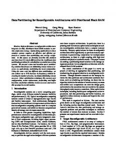
Figure 1 Overview of SDF-based software synthesis.
high level code quite often [13]. This fact demonstrates the efficacy to explore arrays at the high level language level, which we explore in this paper as well.
3
Problem Formulation
Given a set of variables along with the size, we would like to calculate an optimum bank assignment. It is assumed that there are two homogeneous memory banks of equal capacity. This assumption is practical and similar architectures can be found in products such as the Motorola DSP56000, NEC µ PD77016, and Analog Devices ADSP2100. Each bank can be independently accessed in parallel. Such parallelism for memories enhances execution performance. The problem then is to compute a bank assignment with maximum simultaneous memory accesses and minimum capacity requirement. To demonstrate an overview of our work, an SDF-based software synthesis process is drawn in Figure 1. First, applications are modeled by SDF graphs, which are effective at representing multirate signal processing systems. Scheduling algorithms are then employed to calculate a proper actor execution order. The order has significant impact on actor communication buffer sizes and makes scheduling a non-trivial task. For scheduler selection, APGAN and GDPPO are proven to reach certain lower bounds on buffer size if they are achievable [5]. Possible simultaneous memory accesses, partitioning constraints in the figure, together with actor communication buffer sizes and local state variable sizes in actors are then passed as inputs to data partitioning. Our focus in this paper is on the rounded rectangle part in Figure 1. One important consideration is that scalar variables are not targeted in this research. Mostly, they are translated to registers or immediate values. Compilers generally do so to promote execution performance. Memory cost is primarily due to arrays or consecutive data. As we described earlier, therefore, scalar variables and registers are often managed together. Since we are addressing data partitioning at the system design level, consecutive-data variables at a higher level in the compilation process are our major concern in this work.
The description above can be formalized in terms of graph theory. First, we build an undirected graph, called a conflict graph (e.g., see [7][11] for elaboration), G = ( V, E ) , where V and E are sets of nodes and edges respectively. Variables are represented by nodes and potential parallel accesses by edges. There is an integer weight w ( v ) associated with every node v ∈ V . The value of a weight is equal to the size of the corresponding variable. The problem of bank assignment, with two banks, is to find a disjoint bi-partition of nodes, P and Q , with each associated to one bank. The subset of edges with end nodes falling in different partitions is called an edge cut. Edge cut χ is formally defined as χ = { e ∈ E ( v' ∈ P ) ∧ ( v'' ∈ Q ) } where v' and v'' are endpoints of edge e . Since a partition implies a collection of variables assigned to one bank, elements of the edge cut are the parallel accesses that can be carried out. Conversely, parallel accesses are not permissible for edges that do not fall in the edge cut. We should note that edges in the conflict graph represent possible parallelism in the application, and are not always achievable in any solution. Therefore, the objective is to maximize the cardinality of χ . The other goal is to find minimum capacity requirement. Because of homogeneous size in both banks, we aim at storage balancing as well. That is, the capacity requirement is exactly the largest space occupation of either bank. Let C ( P ) denote the total space cost of bank P . It is defined as C(P) =
∑ w(v) .
∀v ∈ P
Cost C ( Q ) is defined in the same way. The objective is to reduce the capacity requirement M under the constraints of C ( P ) ≤ M and C ( Q ) ≤ M . In summary, we have two objectives to optimize the partitioning problem: min ( M ) and max χ .
(1) Though there are two goals, priority is given to max χ in decision making. When there are contradictions between the objectives, a solution with maximum parallelism is chosen. In the following, we work on parallelism exploration first and then on examination of capacity. Alternatively, parallelism can be viewed as a constraint to fit. This is the view taken in the ILP approach proposed later. Variables can be categorized as two types. One is actor communication buffers and the other is state variables local to actors. Buffers are for message passing in dataflow models and management over them is important for multirate applications. SDF offers several advantages in buffer management. One example is space minimization under single appearance scheduling constraint. As mentioned earlier, the APGAN and GDPPO algorithms in [5] are proven to reach a lower bound on memory requirements under certain conditions. However, buffer size is not our primary focus in this work though we do apply APGAN and GDPPO as part of the scheduling phase. The other type, state variables, is local and private to individual actors. State variables act as internal temporary variables or parameters in implementation and are not parts of dataflow expression. In this paper, however, variables are not distinguished by types. Types are merely mentioned to explain the source of variables in dataflow programs.
(a)
(b)
Figure 2 Features of conflict graph connected components extracted from real appli-
cations. (a) short chains (b) trivial components, single nodes without edges.
4
Observations on Benchmarks
We have found that benchmarks, in the form of conflict graphs, derived from several applications (provided in section 6) have sparse connections. For example, a convolution actor involves only two arrays in simultaneous accesses. Other variables to maintain temporary values, local states, loop control, etc. are not apparently beneficial, though no harm is inflicted either, if they are accessed in parallel. Connected components (abbreviated as CGCC, Conflict Graph Connected Component) of benchmarks also tend to be acyclic and bipartite. We say a graph is bipartite if the node set can be partitioned into two sets such that all edges are with end nodes falling in distinct node partitions. This is good news to graph partitioning. Most of them have merely two nodes with a connecting edge. For those a bit more complicated, short chains account for the major structure. There are also many trivial CGCCs containing one node each and no edges. Typical topologies of CGCCs are illustrated in Figure 2 and an example is in Figure 3. Variable singalIn in Figure 3 is an input buffer of the actor and its size is to be decided by schedulers. Variables like hamming and window are arrays internal to the actor. For each iteration of the loop, signalIn and hamming are fetched to complete the multiplication and qualify for parallel accesses. The characteristic of loose connectivity appears to high level relationships among consecutive-data variables. Though we did not investigate characteristics of the connectivity in the scalar case, it is believed that the connectivity is much more complicated than what we observe for arrays. In [7], though, the authors mention that the whole graph may not be connected and multiple connected components exist, and a heuristic approach is adopted to cope with complex topologies of the connected components. The topologies derived in [18] should be even more intricate because more factors are con#define N 320 float hamming[N]; float window[N]; for (m = 0; m < N; m++) { window[m] = signalIn[m] * hamming[m]; }
signalIn hamming (320) window (320)
Figure 3 A conflict graph example of an actor that windows input signals.
sidered. Readers are reminded here once again that only arrays are focused on at high level in our context of combined memory minimization and data partitioning. Another contribution to loose connectivity lies in the nature of coarse-grain dataflow graphs. Actors of dataflow graphs communicate with each other only through communication buffers represented by edges. State variables internal to an actor are inaccessible and invisible to that of other actors. This feature forces modularity of dataflow implementation and causes numerous CGCCs. Moreover, except for communication buffer purposes, any global variables are disallowed. This prevents their occurrences in arbitrary numbers of routines and hence reduces conflicts across actors. Furthermore, based on our observations, communication buffers contribute to conflicts mostly in read accesses. In other words, buffer writing is usually not found in parallel with other memory accesses. The phenomenon is natural in single assignment semantics. In [3], to facilitate memory bank disambiguation, information about aliased memory references is required. To determine aliases, pointer analysis is performed. The analysis results are then represented by a directional bipartite graph. The graph nodes could be memory reference operations or physical memory locations. The edges are directed from operations to locations to indicate dependencies. The graph is partitioned into connected components, called Alias Equivalence Classes (AEC), where any alias reference can only occur in a particular class. AECs are assigned to RAW tiles so that tasks are done independently without any inter-tile communication. Figure 4 is given to illustrate the concept of AECs. For the sample C code in (a), variable b is aliased by x. Memory locations and referencing code are expressed by a directional bipartite graph in (b). Parenthesized integers next to variables are memory location numbers (or addresses) and b and x are aliased to each other with identical location number 2. The connected component in (b) is the corresponding AEC of (a). A relationship exists between AEC and CGCC, keeping in mind that conflict edges indicate concurrent accesses to two arrays. All program instructions issuing accesses to either array are grouped to an identical alias equivalence class. Therefore, both arrays can be found exclusively in that class. In other words, the node set of a CGCC can appear only in a certain single AEC instead of multiple ones. Take Figure 4 as an example. The node set in (c) can be found only in the node set of (b). For an application, therefore, the number of CGCCs is greater than or equal to that of AECs. The relationship between AEC and CGCC makes it promising in the automatic derivation of conflict graphs. This is an interesting topic for further work.
c = a[] * b[]; x = b; d = e[] * x[]; (a)
c(3) a(1) b(2) d(4) e(5)
a b
c=a[]*b[]
d=e[]*x[] (b)
e (c)
Figure 4 Example of the relationship between AECs and CGCCs. (a) sample C code
(b) AEC (c) CGCC.
It is found in [3] that practical applications have several AECs. According to the relationship revealed in the previous paragraph, the number of CGCCs is bigger. If the modularity of dataflow semantics is considered, the number is even bigger. The fact of multiple AECs backs our discovery of numerous CGCCs and loose connectivity. However, the counts of AEC are not related to the simple topology, as demonstrated in Figure 2, of CGCC. Due to the feasibility of reducing CGCC from AEC, we believe that the graph structure of CGCC is much simpler than that of AEC.
5
Algorithms
In this section, three algorithms are discussed. The first one is a 0/1 ILP approach, where all ILP variables are restricted to values 0 or 1. The second one is a coloring method, which is a typical strategy from the relevant literature. The third one is a greedy algorithm that is motivated by our observations on the structure of practical, SDF-based conflict graphs. 5.1 ILP In this subsection, a 0/1 ILP strategy [2] is proposed to solve benchmarks with bipartite structure. Constraint equations are made for the bipartite requirement. If the conflict graph is not bipartite, it is rejected as failure. Fortunately, most benchmarks are bipartite according to our observations. On the other hand, the objective min ( M ) in equation (1) is translated to minimizing space cost difference, min C ( Q ) – C ( P ) , due to ILP restriction on single optimization equation. For each array u , there is an associated bank assignment b u to be decided and b u ∈ {0, 1} . Values of b u denote banks, say B P and B Q respectively. A constant integer z u denotes the size of array u . Memory parallelism constraints b u + b y = 1 are imposed if arrays u and y are to be accessed simultaneously and these constraints also act as the bipartite requirement. The constraints guarantee that distinct banks are assigned to the variables. Let us denote D as the capacity exceeding amount of bank B Q beyond B P . That is, D =
∑ zy –
∀y ∈ B Q
∑ zu .
∀u ∈ B P
This equation can be further decomposed as follows.
∑ zy ⋅ 1 +
D =
∀y ∈ B Q
∑ zy by +
=
∀y ∈ B Q
=
∀u
∑ ( zu bu + zu ( bu – 1 ) )
∀u
=
∑ zu ( bu – 1 )
∀u ∈ B P
∑ zy by + ∑ zu ( bu – 1 )
∀y
=
∑ zu ⋅ ( 0 – 1 )
∀u ∈ B P
∑ z u ( 2b u – 1 )
∀u
Finally, we end up with D = 2 ∑ zu bu – ∀u
∑ zu .
∀u
Since the goal is to minimize the absolute value of D , one more constraint D ≥ 0 is also required. 5.2 2-Coloring and Weighted Set Partitioning A traditional coloring approach is partially applicable for our data partitioning problem in equation (1). If colors represent banks, a bank assignment is achieved while the coloring is done. Though minimum coloring is an NP-hard problem, it becomes polynomialy solvable for the case of two colors [9]. However, using a two-coloring approach, only the problem of simultaneous memory access is handled. Balancing of memory space costs is left unaddressed. To cover space cost balancing, it is necessary to incorporate an additional algorithm. Among those integer set or weighted set problems that are similar to balancing costs, weighted set partitioning is chosen in our discussion because it searches for a solution with exact balancing costs. Weighted set partitioning states that: given a finite set A and a size s ( a ) ∈ Z + for each a ∈ A , is there a subset A' ⊆ A such that
∑ s( a) =
a ∈ A'
∑
s( a) ?
a ∈ A – A'
This problem is NP-hard [9]. If conflicts are ignored, balancing space costs can be reduced from weighted set partitioning and therefore balancing space costs with conflicts considered is NP-hard as well (see Appendix A). 5.3 SPF — A Greedy Strategy In this section, we develop a low-complexity heuristic called SPF (Smallest Partition First) for the heterogeneous-size data partitioning problem. Although 0/1 ILP calculates exact solutions, its complexity is non-polynomial, and therefore its use is problematic within intensive design space exploration loops, and for very large applications, it may become infeasible altogether. Coloring and weighted set partitioning each compute partial results. In addition, the efficacy of coloring is on heavily connected graphs. With the observations of loose connectivity in practice, coloring does not offer much contribution. A combination of coloring and weighted set partitioning would be interesting and is left as future work. In this article, the heuristic of SPF is proposed instead that is tailored to the restricted nature of SDF-based conflict graphs. The results and performance will be compared to that of 0/1 ILP and coloring in the next section. A pseudocode specification of the SPF greedy heuristic is provided in Figure 5. Connected components or nodes with large weights are assigned first to the bank with least space usage. Variables of smaller size are gradually filled to narrow the space cost gap between banks. The assignment is also interleaved to maximize memory parallelism. Note that the algorithm is able to handle an arbitrary number of memory banks, and is applicable to non-bipartite graphs. Thus, it provides solutions to any input application with arbitrary bank count.
procedure SPFDataPartitioning input: a conflict graph G = (V, E) with integer node weights W ( V ) and an integer constant K representing the number of banks. output: partitions of nodes B [ 1…K ] . set an array B [ 1…K ] of K node sets (banks). set C to connected components of G . sort C in decreasing order on total node weights. for each connected component c ∈ C get the node v ∈ c with largest weight. call AlternateAssignment( v ). end for output array B [ 1…K ] .
procedure AlternateAssignment input: a node v . set a boolean variable assigned to false . sort B in increasing order on total node weights. for each node set B [ i ] if no u ∈ B [ i ] such that u is a neighbor of v add v to B [ i ] . assigned ← true . quit the for loop. end if end for if assigned = false add v to the smallest set, B [ 1 ] . end if call ProcessNeighborsOf( v ).
procedure ProcessNeighborsOf input: a node v . for each neighbor b of v if node b has not been processed call AlternateAssignment( b ). end if end for
Figure 5 Our data partitioning algorithm (SPF) for consecutive-data variables.
The SPF algorithm achieves a low computational complexity solution. In the pseudocode specification, the procedure AlternateAssignment performs the major function of data partitioning and is called exactly once for every node in a recursive style through ProcessNeighborsOf. First, the bank array B [ 1…K ] is sorted in AlternateAssignment according to present storage usage. After that, internal edges linked to the input node are examined for every bank, keeping in mind that only cut edges are desired. The last step is querying the assignment of neighbor nodes and a recursive call. Therefore, the complexity of AlternateAssignment is O ( K log K + KN + N ) , where N denotes the largest node degree in the conflict graph. Though the practical complexity of N can be O ( 1 ) according to our observations, the worst case is of O ( V ) complexity. In our assumption, K is a constant provided by the system. For the whole program execution, all calls to AlternateAssignment contribute O ( V 2 ) in worst case and O ( V ) in practice. The remaining computations in SPF include strongly connected component decomposition, sorting connected components by total node weights, and building neighbor node lists. Their complexities are O ( V + E ) [19], O ( C log C ) , and O ( E ) , respectively ( C denotes the number of connected components in the conflict graph.). In summary, the overall computational complexity is O ( V 2 ) in worst case and practically O ( max ( V + E , C log C ) ) for several real applications.
6
Experimental Results
Our experiments are performed for all three algorithms: ILP, 2-coloring, and our SPF algorithm. Since all conflict graphs from our benchmarks are bipartite, every edge falls in the edge cut and memory parallelism is maximized by all three algorithms. Therefore, only the capacity requirement is chosen as our comparison criteria. Improvement is evaluated for SPF over 2-coloring, a classical bank assignment strategy. Performance of SPF is also compared to that of ILP to give an idea of the effectiveness of SPF. For ILP computation, we use the solver OPBDP which is an implementation based on the theories of [2]. To decide bank assignment for coloring, the first node of a connected component is always fixed to the first bank and the remaining nodes are typically assigned in an alternate way because of the commonly-found bipartite graph structure. The order in which the algorithm traverses the nodes of a graph is highly implementation dependent and the result depends on this order. Thus, some results may become better while others may become worse if another ordering is tried. However, the average improvement of SPF is still believed to be high since numerous applications have been considered in the experiments with our implementation. A summary of the results is given in Table 1. The first column lists all the benchmarks that were used in our experiments. The second and third columns provide the number of variables and parallel accesses, respectively. Since the benchmarks are in the format of conflict graphs, those two columns represent node and edge counts, too. The fourth to sixth columns give the bank capacity requirement for each of the three algorithms. Capacity reduction for SPF over 2-coloring is placed in the last column as an improvement measure.
Table 1: Summary of the experimental results. variable counts
conflict counts
coloring
SPF
ILP
improvement(%)
analytic
9
3
756
448
448
40.7
bpsk10
22
8
140
90
90
35.7
bpsk20
22
7
240
156
156
35.0
bpsk50
22
8
300
228
228
24.0
bpsk100
22
8
500
404
404
19.2
cep
14
2
1602
1025
1025
36.0
cd2dat
15
7
1459
1343
1343
8.0
dat2cd
10
5
412
412
412
0.0
discWavelet
92
56
1000
999
999
0.1
filterBankNU
15
10
196
165
164
15.8
filterBankNU2
52
27
854
658
658
23.0
filterBankPR
92
56
974
851
851
12.6
filterBankSub
54
32
572
509
509
11.0
qpsk10
31
16
173
146
146
15.6
qpsk20
31
14
361
277
277
23.3
qpsk50
31
16
453
426
426
6.0
qpsk100
31
16
803
776
776
3.4
satellite
26
9
1048
771
771
26.4
telephone
11
2
1633
1105
1105
32.3
Average
19.4
Most of the benchmarks are extracted from real applications in the Ptolemy environment [6]. Ptolemy is a design environment for heterogeneous systems and many examples of real applications are also included. A brief description of all the benchmarks follows. Two of them are rate converters, cd2dat and dat2cd, between CD and DAT devices. Filter bank examples are filterBankNU, filterBankNU2, filterBankPR, and filterBankSub. The first two are two-channel non-uniform filter banks with different depths. The third one is an eight-channel perfect reconstruction filter bank, while the last one is for four-channel subband speech coding with APCM. Modems of BPSK and QPSK are bpsk10-100 and qpsk10-100 with various intervals. A telephone channel simulation is
represented by telephone. Filter stabilization using cepstrum is in cep. An analytic filter with sample rate conversion is analytic. A satellite receiver abstraction, satellite, is obtained from [16]. Because satellite is just an abstraction without implementation details, reasonable synthetic conflicts are added according to our benchmark observations. Table 1 demonstrates the performance of SPF. Not only does it generate less capacity requirement than the classical coloring method does, but also the results are almost equal to the optimality evaluated by ILP. The polynomial computational complexity (see subsection 5.3) is also lower than the exponential complexity of ILP. In our ILP experiments on a 1GHz Pentium III machine, most of the benchmarks finish within a few seconds. However, discWavelet and filterBankPR spend several hours to complete. In contrast, SPF finishes in less than ten seconds for all cases. In summary, SPF is effective both in the results and the computation time.
7
Conclusion
Bank assignment for arrays has great impact both on parallel memory accesses and memory capacity. Traditional bi-partitioning or two coloring strategies for scalar variables cannot be well adapted to applications with arrays. The variety of array sizes complicates memory management especially for typical embedded systems with stringent storage capacity. We propose an effective approach to jointly optimize memory parallelism and capacity when synthesizing software from dataflow graphs. Surprisingly but reasonably, high level analysis presents a distinctive type of graph topology for real applications. Graph connections are sparse and connected components are in the form of chains, bipartite connected components, or trivial singletons. Some possible future works follow. Our SPF algorithm generates results quite close to optimality. We are curious about the efficacy to graphs with arbitrary topology. Sparse connections found in dataflow models also arouses our interests in the applicability to procedural languages like C. Integration of high and low level optimization is also promising. An integrated optimization scheme involving arrays, scalar variables, and registers is a particularly useful target for further study. Automating conflict information through alias equivalence class calculation is a possible future work as well. Another potential work is to reduce storage requirements further by sharing physical space among variables whose lifetimes do not overlap.
Acknowledgement This research was supported by the Semiconductor Research Corporation (2001-HJ905).
References [1] [2]
O. Avissar, R. Barua, and D. Stewart. Heterogeneous Memory Management for Embedded Systems. CASES’01, pp. 34-43, Atlanta, November 2001. Peter Barth. Logic-Based 0-1 Constraint Programming. Kluwer Academic Publishers. 1996.
[3]
[4]
[5] [6]
[7]
[8]
[9] [10] [11] [12]
[13]
[14]
[15] [16] [17]
[18]
[19]
R. Barua, W. Lee, S. Amarasinghe, and A. Agarwal. Compiler Support for scalable and Efficient Memory Systems. IEEE Transactions on Computers, 50(11):1234-1247, November 2001. S. S. Bhattacharyya, R. Leupers, and P. Marwedel. Software synthesis and code generation for DSP. IEEE Transactions on Circuits and Systems -- II: Analog and Digital Signal Processing, 47(9):849-875, September 2000. S. S. Bhattacharyya, P. K. Murthy, and E. A. Lee. Software Synthesis from Dataflow Graphs. Kluwer Academic Publishers. 1996. J. T. Buck, S. Ha, E. A. Lee, and D. G. Messerschmitt. Ptolemy: A Framework for Simulating and Prototyping Heterogeneous Systems. International Journal of Computer Simulation, 4:155-182, April 1994. J. Cho, Y. Paek, and D. Whalley. Efficient Register and Memory Assignment for Non-orthogonal Architectures via Graph coloring and MST Algorithms. LCTES’02-SCOPES’02, pp. 130-138, Berlin, June 2002. S. Frohlich and B. Wess. Integrated Approach to Optimized Code Generation for Heterogeneous-Register Architectures with Multiple Data-Memory Banks. Proceedings of IEEE 14th Annual ASIC/SOC Conference, pp. 122-126, Arlington, September 2001. M. R. Garey and D. S. Johnson. Computers and Intractability. W. H. Freeman. 1979. E. A. Lee and D. G. Messerschmitt. Synchronous dataflow. Proceedings of the IEEE, 75(9):1235-1245, September 1987. R. Leupers and D. Kotte. Variable Partitioning for Dual Memory Bank DSPs. ICASSP, Salt Lake City, May 2001. P. R. Panda. Memory Bank customization and Assignment in Behavioral Synthesis. Proceedings of IEEE/ACM International Conference on Computer-Aided Design, pp. 477481, San Jose, November 1999. P. R. Panda, F. Catthoor, N. D. Dutt, et. al. Data and Memory Optimization Techniques for Embedded Systems. ACM Transactions on Design Automation for Electronic Systems, 6(2):149-206, April 2001. P. R. Panda, N. D. Dutt, and A. Nicolau. On-Chip vs. Off-Chip Memory: The Data Partitioning Problem in Embedded Processor-Based Systems. ACM Transactions on Design Automation of Electronic Systems, 5(3):682-704, July 2000. D. B. Powell, E. A. Lee, and W. C. Newman. Direct Synthesis of Optimized DSP Assembly Code from Signal Flow Block Diagrams. ICASSP’92, 5:23-26, March 1992. S. Ritz, M. Willems, and H. Meyr. Scheduling for Optimum Data Memory Compaction in Block Diagram Oriented Software Synthesis. ICASSP’95, pp. 2651-2654, May 1995. M. A. R. Saghir, P. Chow, and C. G. Lee. Exploiting Dual Data-Memory Banks in Digital Signal Processors. Proceedings of the 7th International Conference on Architectural Support for Programming Languages and Operating Systems, pp. 234-243, October 1996. A. Sudarsanam and S. Malik. Simultaneous Reference Allocation in Code Generation for Dual Data Memory Bank ASIPs. ACM Transactions on Design Automation of Electronic Systems, 5(2):242-264, April 2000. R. E. Tarjan. Depth first search and linear graph algorithms. SIAM Journal on Computing, 1(2):146-160, 1972
Appendix A: NP-Hardness Proof In this section, we establish the NP-hardness of the data partitioning problem addressed in this paper. As described earlier, data partitioning involves both bi-partitioning a graph and balancing of node weights. In other words, it is a combination of graph 2coloring and weighted set partitioning, where the second problem is NP-hard. Therefore, for simplicity, we only prove that balancing node weights is NP-hard. Equivalently, we establish NP-hardness for the special case of data partitioning instances that have no conflicts. The problem of space balancing is defined in section 3 and the objective is to minimize the capacity requirement M . The decision version of the optimization problem is to check whether both C ( P ) ≤ M and C ( Q ) ≤ M hold for a given constant integer M . In the following paragraphs, we demonstrate the NP-hardness reduction from a known NP-hard problem, weighted set partitioning. + Weighted set partitioning states that: given a finite set A and a size s ( a ) ∈ Z for each a ∈ A , is there a subset A' ⊆ A such that
∑ s(a) =
a ∈ A'
∑ s(a) ?
(2)
a ∈ A – A'
The decision version of our space balancing problem can be rewritten as: Given a + set of arrays U , the associated size z ( u ) ∈ Z for every u ∈ U , and a constant integer M > 0 , is there a subset U ' ⊆ U such that
∑ z ( u ) ≤ M and
u∈U'
∑ z(u) ≤ M ?
(3)
u∈U–U'
Now given an instance ( A, s ) of weighted set partitioning, we derive an instance of space balancing by first setting
∑ s( a) (4) a∈A --------------------- . 2 Then, for every element a ∈ A , we can have a corresponding array u and U is the set of all u . Moreover, z ( u ) = s ( a ) for each corresponding pair of u and a . If a subset A' exists to satisfy equation (2), the corresponding U ' also makes equation (3) true. If a subset of arrays U ' exists for equation (3), the corresponding A' also makes (2) true because M =
∑ s( a) +
a ∈ A'
∑ s(a) = ∑ s(a) ,
a ∈ A – A'
a∈A
where
∑ s(a) ≤
a ∈ A'
∑ s ( a ) and
a∈A ---------------------
∑ s(a) ≤
a ∈ A – A'
∑ s( a)
a∈A ---------------------
.
2 2 The above arguments justify the necessary and sufficient conditions of the reduction from equation (2) to (3).