DECOMPOSTION AND DISTRIBUTED COMPUTING Bernd Steinbach Galina Kempe Freiberg University of Mining and Freiberg University of Mining and Technology, Institute of Computer Technology, Institute of Computer Science, D-09596 Freiberg, Germany Science, D-09596 Freiberg, Germany
[email protected] [email protected] Abstract. The aim of this paper is the support of the extreme requirements in circuit design in the future. To design millions of gates we use the basic principle of divide and conquer on several levels. First, the bi-decomposition splits a complex Boolean function into smaller parts. Second, the three function decomposition of Boolean functions reduces the necessary computation expenditure. Third, taking advantages of both types of decomposition, the distribute computing on several computers scales down the necessary computation time. Experimental results speak for the new approaches.
1 Introduction The law, found by Gordon E. Moore in the 60th [5], tells that the number of transistors on an integrated circuit doubles every 18 months. This law is valid since this time and thus in every such short period doubles both, the power of the computers and the requirements for the circuit design as well. There is a gap between the exponential growth of the number of gates and the nearly constant limited number of their inputs. For this reason, Boolean functions depending an many variables must be realized by multilevel circuits [6], [4]. The best design results of incompletely specified Boolean function in terms of high speed, low power consumption and small area are created by method of bi-decomposition [4] (called grouping in [1]). There are several types of strong and weak bi-decomposition. For the aim of this paper it is sufficient to select the strong OR-bi-decomposition. Their structure is shown in figure 1. xa
g(xa, xc) A
f (xa, xb, xc)
xc xb
h(xb, xc) B
OR-gate
Figure 1. Structure of the OR-bi-decomposition.
The support x of the initial function f is divided into three parts: variables xa that feed only into block A, variables xb that feed only into block B, and the common variables xc. By definition, sets xa, xb, and xc are disjoint and only set xc may be empty. Both, function g(xa, xc) of block A and function h(xb, xc) of block B are simpler than function f (xa, xb, xc), because the sub functions depend on a smaller number of variables. Applying the bi-
decomposition recursively to the blocks A and B leads to a compact multilevel circuit. It depends on the function f (xa, xb, xc), whether and for which sets of variables the OR-bidecomposition exist. The probability of this property growths, if the function f (xa, xb, xc) is incompletely specified, that means their value is not defined for d input pattern. All 2d functions can be described by the mark functions for the ON-set q(xa, xb, xc) and the OFFset r(xa, xb, xc). In the set of functions exists at least one OR-bi-decomposable function with the not empty variable sets (xa, xb) iff formula (1) comes true. The Equation (1) means, it is not allowed, that a One (q) is covered by the projection of Zeros (r) both in xa- and xbdirection.
q( x a , x b , x c ) ⋅ max r ( x a , x b , x c ) ⋅ max r ( x a , x b , x c ) = 0 k
xa
k
xb
(1)
This formula must evaluate extremely often; first for several variable sets (xa, xb) on one decomposition level and second recursively for further decompositions. Aside from the maxk – operation [7] many conjunctions are the kernel task. Therefore, it is important to use a data structure, which allows to calculate the conjunction very quickly. The rest of the paper is organized as follows. Section 2 introduces the three function decomposition and the associated conjunction. Section 3 shows how advantages form both decompositions are intensified by distributed computing. Section 4 presents experimental results and section 5 concludes the paper.
2 Three function decomposition General, it is possible to decompose a Boolean function f ( xi , x 0 ) by f ( xi , x 0 ) = g ( xi , h( x 0 )) , (2) where xi is a single variable, and h( x 0 ) a vector of functions not depending on the variable xi. It is well known, that there are vectors h( x 0 ) containing only two functions. For example, the decompositions defined by Shannon or Davio use two h( x 0 ) -functions, each. We define three functions f − ( x 0 ) , f 0 ( x 0 ) , and f 1 ( x 0 ) using the cofactors f ( xi = 0, x 0 ) , f ( xi = 1, x 0 ) and the Boolean derivative ∂f ( xi , x 0 ) (3) = f ( xi = 0, x 0 ) ⊕ f ( xi = 1, x 0 ) ∂xi Definition: The decomposition functions of a function f ( xi , x 0 ) are defined as follows:
∂f ( xi , x 0 ) f ( xi , x 0 ) , ∂xi ∂f ( xi , x 0 ) Zero Function: f ( xi = 0, x 0 ) , f 0 (x0 ) = ∂xi ∂f ( xi , x 0 ) f 1(x0 ) = f ( xi = 1, x 0 ) . One Function: ∂xi The original function can be computed as a decomposition into three functions. Theorem 1: Every function f ( xi , x 0 ) can be decomposed by:
Stroke Function:
f − (x0 ) =
f ( x i , x 0 ) = f − ( x 0 ) ∨ x i f 0 ( x 0 ) ∨ xi f 1 ( x 0 )
(4)
Note, the sub functions f 0 ( x 0 ) , and f 1 ( x 0 ) are different from the cofactors f ( xi = 0, x 0 ) , f ( xi = 1, x 0 ) and, possess the following essential property.
Theorem 2: Each pair of the functions f − ( x 0 ) , f 0 ( x 0 ) , and f 1 ( x 0 ) is disjoint.
f α ( x 0 ) ⋅ f β ( x 0 ) = 0 , for α , β ∈ {−, 0, 1} and, α ≠ β (5) Because of theorem 2, the OR-operations in (4) can be replaced by EXOR-operations. If the functions f1 ( xi , x 0 ) and f 2 ( xi , x 0 ) are decomposed by (4) into the component functions −
0
−
1
0
1
f1 ( x 0 ) , f1 ( x 0 ) , f1 ( x 0 ) and f 2 ( x 0 ) , f 2 ( x 0 ) , f 2 ( x 0 ) respectively, special algorithms −
for the Boolean operations are needed. For example, the component functions f 3 ( x 0 ) , 0
1
f 3 ( x 0 ) , f 3 ( x 0 ) of the conjunction f 3 ( xi , x 0 ) = f1 ( xi , x 0 ) ⋅ f 2 ( xi , x 0 ) are computed as follows: − − − f 3 = f1 f 2 (6) 0
−
0
1
−
1
−
0
0
f 3 = f1 f 2 ∨ f1 f 2 ∨ f1 f 2 1 1
−
1 1
0
(7)
1
f 3 = f1 f 2 ∨ f f 2 ∨ f f 2 (8) It seems, that the calculations of 7 conjunctions of sub functions are more complex than one conjunction of the given functions. But the decomposition of each function into three parts reduces theoretically and practically (see section 4) the necessary computation time. All other Boolean operations based on the thee function decomposition are described in [3].
3 Distributed computing The three function decomposition has very good properties for distributed computing of the conjunction. The main expenditure to compute the conjunction using the formulas (6), (7) − − − 0 0 − 0 0 and (8) consists in the calculation of the conjunctions f1 f 2 , f1 f 2 , f1 f 2 , f1 f 2 , −
1
−
1
1
1
f1 f 2 , f1 f 2 , and f1 f 2 . The calculations of all 7 conjunctions are independently from each other. Consequently, it is possible to execute these 7 calculations in parallel. The 0 1 disjunctions f 3 = h1 ∨ h2 ∨ h3 and f 3 = h4 ∨ h5 ∨ h6 , are independently too. It follows from theorem 2, that the disjunctions in the formulas (7) and (8) are realizable in a constant time. The component functions are disjoint, thus in order to calculate the disjunctions, their simple chaining is enough. Therefore is not necessary to calculate the disjunctions in parallel. Figure 2 shows the operations, which can be calculated in parallel. −
−
f 3 = f1 f 2
−
−
h1 = f1 f 2
0
0
h2 = f1 f 2
−
0
h3 = f 1 f 2
0
−
h4 = f1 f 2
1
1
h5 = f1 f 2
−
1
h6 = f1 f 2
0
f 3 = h1 ∨ h2 ∨ h3 1
f 3 = h4 ∨ h5 ∨ h6 Figure 2. Parallel computing of tuple conjunction.
Here, the distributed computing based on the Client-Server-Model. The data communication between client and server takes place on the basis of the Socket Interface BSD UNIX [2] using the Transmissions Control Protocol (TCP). Since there are a synchronization of data exchange between sender and receiver, a synchronous remote service invocation (SRSI) is used [8].
1
client
servers
create of connection
job 1 first allocations of jobs
server 1
job 1
data exchange by sockets create of connection
job 2 job 2 data exchange by sockets
next allocations
job 3
create of connection
server 2
job 3 data exchange by sockets son processes
final calculation father process
son processes
father process
create of son processes of client create of son processes of server data exchange by pipes
Figure 3. Overview of interaction between client and servers.
Figure 3 shows the interaction between the client and e.g. two servers in order to calculate one conjunction distributed using several servers. After the start, the client call for services to several servers in parallel. For this, the client starts several son processes and every son process of the client communicates to exactly one server. The life cycle of son process includes the time of the data transmission and the operating time to calculate the conjunction of one pair of sub functions on one server. After the back transfer of the result data to the client the respective son process of the server will be terminated. If the son process of the client has received the result data, a message is transmitted using a control pipe to the waiting father process. The transfer of the results will be done by a process specific data pipe to the father process immediately after the receiving of the message. Usually, the number of jobs is larger than the number of available servers. The transfer of the next job to a free server will be realized by the same procedure, described above. The calculation of the final result will be done after the successful termination of the last partial calculation. It is possible to overlap the back transfer of the data from the server and the start of the next partial calculation. Experimental results shown, that this is not necessary, because the transmission time is very short in the comparison to the computation time. It is well know, that the distributed computing needs additional expenditures. There are:
• • •
the data exchange between the client and servers by sockets; the data transfer from son to father process of the client; the creating of processes of the client and servers.
Therefore, it is obvious, that the Boolean operations, using distributed computing, are faster than usual Boolean operations only for the Boolean functions larger than a certain size. The fastest distributed calculation is given, if there exist a particular server for each
job, all servers have the same power and, all jobs are equal in the size. If some servers differs in their power or some jobs have different size then the total calculation time depends on the time of the most slowly pair job - server and some other server are waiting. If the number of servers is smaller than the number of jobs, an optimization is possible in such a way, that the jobs are sorted from large to small sizes. After the termination of a job the free server gets the largest job from the queue. Thus the smallest job is computed last and the waiting time is reduced. Additional to the distributed computing of the conjunction based on the three function decomposition, it is possible to check the OR-bi-decomposition for one or more pairs of sets of variables xa and xb in parallel. If the mark functions q and r are represented by the three function decomposition each evaluation of (1) needs 14 conjunction of component functions, thus 14 distributed jobs are necessary. In parallel, the client calculates the maxk operations, selects the sets of variables xa and xb and controls the distributed computing. A complete check of one incompletely specified function for the OR-bi-decomposition required the computation of much more jobs compared with the distributed computation of one conjunction based on the three function decomposition. Thus, a lager number of servers can be utilize efficiently.
4 4.1
Experimental Results Three-function decomposition
To verify the feasibility of three-function decomposition, random functions depending on 14 input variables are designed, and decomposed into three subfunctions according to (4). The original function and the sub functions are represented as optimized sums of disjoint cubes [7]. Figure 4 shows the processing time for computation of the conjunction of two random functions in case of the three function decomposition and the original function as well. The calculation of the conjunction of two random functions decomposed in the three function representation need less time for all random functions (approximately one half to one third) as the one function representation. The experiments shown, that the three function representation is faster in processing time for functions with many products. 7,00
5,00 4,00
1 Func.
3,00
3 Func.
2,00 1,00 6126
6014
5805
5451
5362
5087
4847
4627
4202
3726
3269
2458
1462
0,00 256
Time (sec.)
6,00
Avarage Number of Cubes
Figure 4. Computation time of conjunctions on one computer.
4.2
Distributed computing of conjunction
The practical measurements based on four UNIX-Workstation on different levels of power. Random functions are decomposed having 20 input variables and representing as optimized sums of disjoint cubes [7]. Table 1. Calculation of conjunctions of three function representation using up to four computers.
Number of Cubes Time of Calculation (sec) Reduction (%) 1st Func. 2nd Func. sequential 2 Server 3 Server 4 Server 2 Server 3 Server 4 Server 6.844 6.966 5 10 10 10 -100 -100 -100 16.503 16.798 22 28 28 24 -27 -27 -9 30.372 30.341 109 92 88 74 16 19 32 72.580 73.526 562 378 321 327 33 43 42 121.663 121.390 1.282 805 666 646 37 48 50 171.161 171.637 2.113 1.327 1.097 966 37 48 54 221.095 221.306 2.952 1.858 1.453 1.269 37 51 57 267.380 268.208 3.726 2.365 1.640 1.470 37 56 61 311.722 313.228 4.438 2.440 1.994 1.917 45 55 57 352.719 354.462 5.031 2.878 2.323 2.178 43 54 57 391.298 391.227 5.493 3.087 2.527 2.368 44 54 57 425.420 424.962 5.830 3.172 2.625 2.452 46 55 58 Sum 31.562 18.440 14.772 13.701 42 53 57
Table 1 shows the processing time for computation of the conjunction of two random functions. Already the results using two servers show, that the distributed computing speeds up only for functions larger than a certain size. The calculation time in case of distributed computing compared to the sequential computing sinks for the examined functions up to 54% (reduction is 46%). The theoretical optimum of reduction in case of two computers is 50%. Table 1 shows, that a rising function size approximates the practical reduction to the theoretical reduction. Due to the Amdahl’s law, the theoretical optimal reduction is not reachable, because the distributed computing includes sequential parts and needs some additional expenditures. The use of some additional servers leads to further reduction of the computation time. Compared to sequential computing, the average time reduction is 42% using two servers, 53% using three servers, and 57% using four servers. The additional reduction of each further server sinks. The reason for this is relatively small number of jobs. Measurements of the additional expenditures show, that the time of the data exchange between client and server is very small compared with the total computing time. The average value of the time for data exchange to the total computing time is 0,28%. The data transfer between father and son processes is necessary in one direction only and runs in parallel with the calculation. The time for creating of processes is smaller 1 s per process. Thus, these two factors can be neglected in comparison with the total computing time. 4.3
OR-bi-decomposition
Table 2 shows the processing time which is necessary to find of the maximal sets of variables x a and x b for an OR-bi-decomposition of incompletely specified function, represented with the mark functions q (x) and r (x) .
Table 2. Computation time for distributed OR-bi-decomposition.
Num . of Var. 18 19 20
ReducNumber of Time of Time of Calculation Reduction Cubes Calculation (sec) tion (sec) (%) (%) 2 Serv 3 Serv 4 Serv 2 Serv 3 Serv 4 Serv r (x) 1 Func. 3 Func. q(x) 51091 43185 24240 6483 73,3 6075 4852 3457 6,3 25,2 46,7 94836 96394 123886 31202 74,8 24146 19004 13772 22,6 39,1 55,9 64749 91169 56685 21938 61,3 16643 11937 9888 24,1 45,6 54,9
The mark functions q (x) and r (x) are represented by optimized sums of disjoint cubes [7] for both, by one function and decomposed into three function. Table 2 shows, based on the three function representation the calculation of the OR-bi-decomposition is much faster. Using the three function decomposition and one computer the calculation time of the ORbi-decomposition is reduced to nearly one third. Compared to a single conjunction, the increase of the number of computers leads to a significant increase of the reduction for distributed computing of the OR-bi-decomposition. The reason of this fact is, that the larger number of jobs improves the load balancing.
5 Conclusion The OR-bi-decomposition of large incompletely specified Boolean function and their application in circuit design is the background for a number of new results. First, the conjunction of Boolean functions is the most time consuming operation for this task. Second, the three function decomposition speed up the calculation of the conjunction. Third, in order to calculate a conjunction three function decomposition needs 7 simpler conjunctions, which can calculated in parallel. Fourth, preferring a good load balancing, the calculation of the conjunction of three function representation should distributed only to a small number of computers. Fifth, the OR-bi-decomposition itself allow on a higher level the efficient distributed computing using a lager number of computers. Finally, the experimental results show, that all suggested approaches should be combined.
6 References [1] Bochmann, D.; Dresig, F.; Steinbach, B.: A new Decomposition Method for Multilevel Circuit Design. in European Conference on Design Automation, Amsterdam, The Netherlands, 1991, pp. 374–377. [2] Comer, D. E., Stevens, D. L.: Internetworking with TCP/IP, Vol.III, Client-Server Programming and Application, Englewood Cliffs, Prentice Hall, 1993. [3] Kempe, G., Lang, Ch.,: Efficient Representation of Boolean Functions by Three- and Four-Function Decomposition, in Proc. Workshop Boolean Problems, Freiberg, pp.39-46, 1998. [4] Mishchenko, A., Steinbach, B., Perkowski, M.: An Algorithm for Bi-Decomposition of Logic Functions. DAC 2001, Las Vegas (Nevada) USA, pp.103-108. [5] Moore, G. E.: Cramming more components onto integrated circuits. Electronics, Volume 38, Number 8, April 19, 1965. [6] Sasao, T. ed.: Representation of Discrete Functions, Kluwer Academic Publishers, May 1996. [7] Steinbach, B.: XBOOLE - A Toolbox for Modelling, Simulation, and Analysis of Large Digital Systems. System Analysis and Modelling Simulation. Gordon & Breach Science Publishers, 9(1992), Number 4, pp. 297 – 312. [8] Weber, M.: Verteilte Systeme, Spektrum Akademischer Verlag GmbH, Heidelberg Berlin, 1998.