Herbert Edelsbrunner for kindly hosting me at the Duke University ..... NVIDIA Fermi GPU architecture and available in affordable consumer graphics cards ...... sizeable portion of the CPU is dedicated to the many levels of a cache hierarchy.
DELAUNAY TRIANGULATION IN R3 ON THE GPU
ASHWIN NANJAPPA (B.Eng. (Comp. Sci.), Visvesvaraya Technological University, India)
A THESIS SUBMITTED FOR THE DEGREE OF DOCTOR OF PHILOSOPHY DEPARTMENT OF COMPUTER SCIENCE NATIONAL UNIVERSITY OF SINGAPORE 2012
To mom and dad, for their love and support.
To my loving wife Prithvi, for her patience and understanding.
Acknowledgements This work would not have been possible without the help and support of many people. First and foremost, I would like to thank my advisor Prof. Tan Tiow Seng for taking me under his wing and guiding me along this long and eventful journey. His kind words of encouragement and moral support carried me through the many trying times of my PhD. Without his personal interest, mentoring and valuable feedback, this work could not have been accomplished. I am grateful to Prof. Herbert Edelsbrunner for kindly hosting me at the Duke University and the Institute of Science and Technology, Austria and lending an ear to my research problem. Prof. Kok-Lim Low and Prof. Alan Cheng Ho-Lun gave helpful feedback on my research during weekly lab meetings and also graciously accepted to be my examiners. I am thankful to Dr. Huang Zhiyong for supporting me with a postgraduate research internship at the Institute of Infocomm Research, Singapore. Among my colleagues, I am most grateful to Cao Thanh Tung for selflessly sharing his knowledge, for enriching my research with his collaboration and for the innumerable deep discussions we have had about every topic under the Sun. Gao Mingcen and Qi Meng have always been very kind, helpful and they graciously agreed to review early drafts of this thesis. My friends Poonna Yospanya, Tang Ke, Su Jun, Alvin Chia, Lai Kuan, Jiayan Guo, Li Ruoru, Son Hua, Yang Ke, Sang Ngoc Le, Shamima Banu, Li Yunzhen, Srinivasan Sridharan, Ge Shu, Calvin and Guodong made my years at the lab intellectual, fun and colorful. I am also thankful to Wang Lu and Fangxiao for their friendship and support during my stay at Shandong University, China. Tsung-Han Chiang, Harish Katti, Ankit Goel, Saurabh Garg, Amit Bansal and Sriganesh Srihari undertook the same journey as me and I am indebted to them for sharing their friendship, experience and support. I am also thankful to Shivakumara, Merina Ranjith, Parineeth, Bharani Gopinath, Amit Goenka, Vinay Kamath, Tarun Maheshwari and all my other friends for their support and encouragement all these years. Finally, teaching at the School of Computing has been one of the best experiences of my life and I thank Prof. Stanislaw Jarzabek, Yinxing Xue and Christina Carbunaru for their support. I am grateful to the hundreds of students who I was lucky enough to meet in CS3215, CS3201, CS3202, CS2103 and CS1101C. The joy of teaching them kept me going through the ups and many downs of my PhD.
v
Abstract The Delaunay triangulation of points in R3 is a fundamental computational geometry structure that is useful for representing and studying objects from the physical world. The 3D Delaunay triangulation has desirable qualities that make it useful in many applications like FEM, surface reconstruction and tessellating solids. Algorithms for 3D Delaunay have been devised that utilize a multitude of techniques and are suitable for single and multi-core CPUs and distributed memory systems. With the ubiquity of the GPU in cellphones, tablets, workstations and cloud computers, there has been a growing interest in 3D Delaunay triangulation algorithms for the GPU. This thesis presents 3D Delaunay triangulation algorithms that effectively utilize the massive parallelism of the GPU. The gFlip3D algorithm is designed to enable massively parallel point insertion and flipping in 3D on the GPU. The algorithm achieves a high level of parallelism performing one point insertion per thread and one flip operation per thread. For any type of input, less than 0.0001 of the facets in the output from this algorithm are not locally Delaunay. The CUDA implementation of this algorithm achieves a speedup of up to 6 times over the 3D Delaunay triangulator of CGAL. To provide a better quality triangulation as input to massively parallel flipping algorithms, this thesis examines the coloring and dualization of the digital grid in R3 . We show that it is difficult to color a digital grid in 3D such that the dualized triangulation is topologically and geometrically valid. We also show that dualizing a 3D digital Voronoi vertex is not possible. As an alternative technique, we demonstrate the utility of grid perturbation to coloring and dualization so that a triangulation can be obtained from it. This thesis presents the gStar4D algorithm that constructs the 3D Delaunay triangulation by using the neighbourhood information in the digital grid as an approximation of the Delaunay triangulation. It achieves this by the massively parallel creation of stars of each input point lifted to R4 and the use of an unique star splaying approach to splay these 4D stars in parallel and make them consistent. The result is a convex hull of the lifted points and the 3D Delaunay triangulation can be obtained from its lower hull. The algorithm introduces a concept of reciprocated insertions that simplifies the inconsistency handling and an elegant technique to find the confinement proof of a point in a star. The CUDA implementation of gStar4D achieves a speedup of up to 5 times over the 3D Delaunay triangulator of CGAL. gDel3D is a heterogeneous GPU-CPU algorithm that repairs the near-Delaunay output of gFlip3D using a conservative star splaying approach on the CPU to obtain the 3D Delaunay triangulation. Stars are created only for the points in non-locally-Delaunay facets by using working sets from the triangulation. The star splaying approach conservatively creates other stars directly from the triangulation and once they are consistent repairs only the affected
vii
viii
portion of the triangulation to obtain the 3D Delaunay triangulation. Our implementation of gDel3D achieves a speedup of up to 6 times over the 3D Delaunay triangulator of CGAL. The running time of gDel3D includes both the time taken by gFlip3D and that for fixing its output to Delaunay. The massively parallel techniques presented in this thesis are not only useful for 3D Delaunay triangulation, but can be extended and adopted to solve other computational geometry problems in R3 and R4 using the GPU. To demonstrate this, we extend the star splaying concepts of gStar4D and gDel3D algorithms to devise the gReg3D algorithm that can construct the 3D regular triangulation on the GPU. This algorithm allows stars to die, finds their death certificate and uses methods to propagate this information to other stars. The implementation of this algorithm achieves a speedup of up to 4 times over the 3D regular triangulator of CGAL. We also explore the concept of non-optimal flipping as a means to improve the quality of triangulation constructed from massively parallel point insertion. The algorithms described in this thesis show that the massive parallelism of the GPU can be harnessed to construct the Delaunay and regular triangulation in R3 for all types of inputs. We also show that these techniques can be adapted easily to solve other computational geometry problems in R3 and R4 using the GPU. This thesis also contributes the optimized and robust implementation in CUDA of all its algorithms that can be used with all types of inputs. This is made freely available on the internet to anybody from the scientific and engineering community. With these contributions this thesis lays the foundation for further work on computing the 3D Delaunay triangulation on the GPU.
Contents List of Algorithms 1 Introduction
xiii 1
1.1
Delaunay triangulation in our world
1
1.2
Massive parallelism for everyone
2
1.3
Motivation
3
1.4
Contribution
4
1.5
Outline
5
2 Background 2.1
2.2
Computational geometry
7 7
2.1.1
Preliminaries
7
2.1.2
Convex hull
9
2.1.3
Voronoi diagram
10
2.1.4
Delaunay triangulation
12
2.1.5
Duality relationship
14
2.1.6
Lifted relationship
15
2.1.7
Flipping
16
Compute on the GPU
19
2.2.1
A walk down the graphics pipeline
19
2.2.2
CUDA Programming Model
22
2.2.3
CUDA Challenges
23
2.2.4
Summary
25
3 Related Work
27
3.1
Approaches
3.2
Sequential algorithms
28
3.2.1
Edge flip algorithm
28
3.2.2
Incremental search algorithms
30
3.2.3
Divide-and-conquer algorithms
31
3.2.4
Sweep algorithms
34
3.2.5
Incremental insertion algorithm
35
3.2.6
Summary
40
3.3
27
Parallel Algorithms
42
3.3.1 3.3.2
Algorithms for abstract parallel architectures Distributed memory algorithms
42 43
3.3.3
Multi-core CPU algorithms
47
3.3.4
GPU algorithms
49
3.4
Implementations
53
3.5
Summary
54
ix
Contents
x
4 gFlip3D: Flipping in R3 on the GPU
55
3
55
4.1 4.2
4.3
4.4
4.5
Flipping in R
The gFlip3D algorithm
58
4.2.1
Parallel point insertion
59
4.2.2
Parallel flipping
64
Data structures
68
4.3.1
Triangulation
68
4.3.2
Initial triangulation
72
4.3.3
Point-Tetrahedron association
73
Implementation
73
4.4.1
Predicates
73
4.4.2
Array expansion
76
4.4.3
Sort uninserted points
77
Analysis
77
4.5.1
Setup
77
4.5.2
Input
78
4.5.3
CGAL
78
4.5.4
Quality
82
4.5.5
Running time
83
4.5.6
Speedup over CGAL
84
4.5.7
Time breakdown
84
4.5.8
Point insertion
87
4.5.9
Flipping
88
4.5.10 Terminal flipping 4.6 5
89
4.5.11 Summary
90
Conclusion
90
Dualization and coloring in R3 5.1 5.2
5.3
5.4
5.5
Introduction Coloring and dualization in R 5.2.1
Preliminaries
5.2.2
Dualization
91 91
2
91 92 92
Dualization in R3
93
5.3.1
Preliminaries
93
5.3.2 5.3.3
Problem Grid perturbation
94 94
Coloring in R3
96
5.4.1
Topology and geometry
96
5.4.2
Flooding
97
5.4.3
Topology checks
98
5.4.4
Uncolored voxels
100
5.4.5
Orientation check
101
5.4.6
Boundary and convexity
103
Conclusion
6 gStar4D: Star splaying in R4 on the GPU
105 107
Contents
xi
6.1
Star splaying in R4
107
6.2
The gStar4D algorithm
109
6.3
6.4
6.5
6.2.1
Data structures
109
6.2.2
Algorithm description
109
6.2.3
Stage 1: Construct digital Voronoi diagram
111
6.2.4
Stage 2: Create working sets
111
6.2.5
Stage 3: Create stars
114
6.2.6
Stage 4: Make stars consistent
117
6.2.7
Stage 5: Get tetrahedra from stars
119
Implementation
120
6.3.1
Stars
120
6.3.2
Insertion history table
123
6.3.3
Finding confinement proof
123
6.3.4
Sorting input points
126
Analysis
126
6.4.1
Running time
126
6.4.2
Speedup
128
6.4.3
Grid size
129
6.4.4
Time breakdown
130
6.4.5
Insertions
131
Conclusion
7 gDel3D: A hybrid GPU-CPU algorithm for 3D Delaunay
133 135
7.1
Repairing a near-Delaunay triangulation
135
7.2
The gDel3D algorithm
136
7.2.1
Stage 1: gFlip3D
139
7.2.2
Stage 2: Create stars for failed points
139
7.2.3
Stage 3: Collect inconsistencies
139
7.2.4
Stage 4: Process inconsistencies
140
7.2.5
Stage 5: Update triangulation
141
7.3
7.4
Analysis 7.3.1
Running time
141
7.3.2
Speedup
143
7.3.3
Repair time
145
7.3.4 7.3.5
Number of stars Time breakdown
146 147
Conclusion
8 Extensions 8.1
8.2
141
148 151
gReg3D: Regular triangulation in R3 on the GPU
151
8.1.1
Background
151
8.1.2 8.1.3
The gReg3D algorithm Analysis
152 156
8.1.4
Summary
161
Extending the terminal flipping method
161
8.2.1
162
Removing unflippable facets with non-optimal flips
Contents
xii
8.2.2
Extended terminal flipping approach
164
8.2.3
Analysis
165
8.2.4
Summary
166
9 Conclusion
167
List of Algorithms 1
Edge Flipping . . . . . . . . . . . . . . . . . . . . . . . . . . . . . . . . . . . . . . . . .
29
2
Incremental search algorithm . . . . . . . . . . . . . . . . . . . . . . . . . . . . . . . .
31
3
Incremental insertion algorithm . . . . . . . . . . . . . . . . . . . . . . . . . . . . . . .
35
4
Flipping after each insertion . . . . . . . . . . . . . . . . . . . . . . . . . . . . . . . . .
37
5
Bowyer-Watson method . . . . . . . . . . . . . . . . . . . . . . . . . . . . . . . . . . .
39
6
gFlip3D algorithm . . . . . . . . . . . . . . . . . . . . . . . . . . . . . . . . . . . . . .
58
7
gStar4D algorithm . . . . . . . . . . . . . . . . . . . . . . . . . . . . . . . . . . . . . . 110
8
Finding confinement proof in R4 . . . . . . . . . . . . . . . . . . . . . . . . . . . . . . 125
9
gDel3D algorithm . . . . . . . . . . . . . . . . . . . . . . . . . . . . . . . . . . . . . . .
10
gReg3D algorithm . . . . . . . . . . . . . . . . . . . . . . . . . . . . . . . . . . . . . . 153
11
Finding death certificate in R4 . . . . . . . . . . . . . . . . . . . . . . . . . . . . . . . 155
12
Extended terminal flipping
. . . . . . . . . . . . . . . . . . . . . . . . . . . . . . . . .
137
164
xiii
Chapter
1
Introduction 1.1
Delaunay triangulation in our world
One of the principal uses of a computer is to help us study and understand our physical world. Computers are used to represent and process everything from microscopic protein molecules to the objects we manufacture to the large geological structures of our planet. All these entities exist in three dimensions (3D) and to perform computation on them we need algorithms to discretize them and represent them as triangulations and meshes. An object in the physical world is converted into a set of points by typically scanning its surface or its interior structure. A triangulation in 3D decomposes the convex hull of these points into a set of tetrahedra, each composed of 4 points. Of the many possible 3D triangulations of the points, a special type called the Delaunay triangulation is popular among both theoreticians and practitioners. The Delaunay triangulation, shown in Figure 1.1, is one of the basic structures in computational geometry. It is intimately connected to two other basic structures: the convex hull and the Voronoi diagram by special relationships (see Section 2.1.5 and 2.1.6). Important geometric graphs like Euclidean minimum spanning tree (EMST) [Sha78], the Gabriel graph [GS69] and the relative neighborhood graph [Tou80], are all subgraphs of the Delaunay triangulation. The 3D Delaunay triangulation has desirable qualities that make it useful in a wide range of applications. Consider its application in scientific computing based on the finite element method (FEM). An essential step in these computations is to find a mesh that properly discretizes the continuous domain with simple elements such as tetrahedra. It is crucial to minimize the numeric and discretization error in such scientific computations, and these errors depend on the geometric shape and qualities of the tetrahedron elements. The 3D Delaunay triangulation is the first choice for building meshes for FEM. One of the properties that makes it desirable is that it minimizes the containment radius of the tetrahedra. The containment radius is defined as the radius of the smallest sphere containing the tetrahedron [Raj94]. This makes the 3D Delaunay triangulation the most compact triangulation, making it invaluable for mesh generation. Another good property is that the faces of the 3D Delaunay triangulation have been proven to have an acyclic visibility depth order when seen from any viewpoint in 3D [Ede89]. This makes them useful for 3D rendering applications. Some of the other uses of 3D Delaunay triangulation are in surface reconstruction [Boi88], molecular modelling and tessellating solid shapes [LS05].
1
Chapter 1. Introduction
2
Figure 1.1: The 3D Delaunay triangulation of points distributed inside a sphere.
1.2
Massive parallelism for everyone
Massive parallelism involves the use of hundreds to thousands of processing elements (PE) to execute thousands to millions of processes or threads simultaneously in order to accomplish a computation. Such massively parallel processor (MPP) computer systems [Bat80] were prohibitively expensive and not accessible to anyone outside of the defence, space and academic organizations. Today, our smartphones, tablets, notebooks and workstations have processors with massively parallel processing capabilities. Consider the NVIDIA GF110 GPU, shown in Figure 1.2, which is based on the NVIDIA Fermi GPU architecture and available in affordable consumer graphics cards like the NVIDIA GTX 580. It has 512 cores running at 1.5 GHz. These cores are distributed among 16 streaming multiprocessors (SM), 32 cores in each SM. The GPU is capable of 1581 GFLOPS compute throughput and a memory bandwidth of 190 GB/sec. It supports the CUDA and OpenCL programming models, both of which allow users to write programs that can launch millions of lightweight threads to process data simultaneously. Massively parallel processors in consumer hardware are not limited to graphics cards alone. Processors from both Intel and AMD used in notebooks and computer workstations have an integrated GPU with hundreds of cores. System-on-chip (SoC) like NVIDIA Tegra 3 that is used in smartphones and tablets also have an integrated GPU with tens of cores. Massively parallel programming models like CUDA and OpenCL are already supported on these processors and are being increasingly supported on these SoC. There is a growing interest in applying the GPU to problems where the parallelism is not obvious and the efficient solution is non-trivial. Many recent GPU algorithms have used novel approaches to solve traditional 2D and 3D computational geometry problems [CTMT10] [QCT12].
1.3. Motivation
3
Figure 1.2: Architecture of the NVIDIA GF110 GPU [Nvi].
1.3
Motivation
The performance of the 3D Delaunay triangulation algorithm determines the efficiency of mesh generators [She96b]. In its other applications too, the Delaunay triangulation is an essential step and often the bottleneck in the overall computation [BMHT99]. Due to its importance, there have been numerous efforts at designing faster and more scalable algorithms for 3D Delaunay triangulation on a wide range of parallel architectures. The first attempts at parallel Delaunay were based on the divide and conquer (D&C) strategy. The input points are spatially partitioned amongst the available processors in a sequential stage. After this, each processor computes the Delaunay triangulation of its set of points simultaneously. Then a merge stage that relies on the ordering of edges incident to a vertex is used to stitch together the pieces of the triangulation. These algorithms worked only in 2D since such an incidence ordering does not exist in three and higher dimensions. Moreover, the divide and the merge stages are complex and sequential. These limitations were overcome by pre-construction of the merge portions of the 3D triangulation in a sequential stage [CMPS93]. The holes left in the triangulation could be filled in parallel. The complex pre-construction stage in such algorithms limits their scalability. As processors with a few (2-16) cores became accessible in the last decade, there has been an interest in multi-core algorithms for 3D Delaunay [KKZ05] [BBK06]. These algorithms begin with a sequential stage where a coarse triangulation is constructed from a subset of the points. The rest of the points are distributed amongst the threads, one thread per CPU core. All the threads attempt to insert one point each into the triangulation. Each thread locks the tetrahedra or vertices that will be deleted by the point insertion. If there is an overlap of the locked regions of any two threads, one of them needs to rollback its operations. These algorithms cannot scale to hundreds or thousands of cores since the probability of contention increases with increase in the number of threads. With the ubiquity of massively parallel GPU processors, there has been a growing interest in geometry algorithms for the GPU. Hoff et al. [HKL+ 99] computed the discrete Voronoi diagram on the GPU.
Chapter 1. Introduction
4
They also mention the possibility of obtaining the 2D Delaunay triangulation from the discrete Voronoi, but report no implementation or performance. The GPU-DT algorithm [RTC08] takes a hybrid GPU-CPU approach to compute 2D Delaunay triangulation. On the GPU, it computes a discrete Voronoi diagram and dualizes it to a triangulation. On the CPU, this is transformed to a 2D Delaunay triangulation by using flipping and by fixing the convex hull. GPU-DT achieves a modest speedup of 2 over the best sequential algorithms. In summary, the classic divide and conquer algorithms are complex in 3D and have limited scalability. Multi-core algorithms to compute 3D Delaunay cannot scale to hundreds of cores due to the increased contention and the resulting expensive locking and rollback operations in their algorithms. There has been a lot of interest in developing GPU algorithms for computational geometry in recent years. The techniques used in algorithms of Hoff and GPU-DT like dualizing a discrete Voronoi diagram and flipping in CPU do not work in 3D and are not trivially portable to the GPU architecture. There is a demand for fast and scalable 3D Delaunay algorithms that can produce exact and robust results. The methods used in current 2D computational geometry algorithms for the GPU cannot be generalized to and do not work in 3D. There is currently no massively parallel algorithm to produce 3D Delaunay triangulation that fills these gaps. In this thesis, we explore some unconventional directions and devise near-Delaunay and Delaunay algorithms in 3D for massively parallel processors like the GPU. These algorithms achieve a high degree of parallelism where millions of geometry operations, one per thread, can be performed simultaneously without requiring complex locking and rollback strategies. These 3D Delaunay algorithms are robust, work efficient, massively parallel and scale with the number of available cores.
1.4
Contribution
Our contributions described in this thesis include: 1. It is well known that flipping to Delaunay works in 3D only with incremental insertion. In our gFlip3D algorithm we devise methods to achieve massively parallel insertion and flipping to get results that are Delaunay or nearly-Delaunay. This kind of triangulation is useful in the field of Delaunay refinement. gFlip3D achieves a speedup of up to 6 times over the best sequential 3D Delaunay implementations. 2. One way to improve the quality of the result of gFlip3D is to start with a good quality coarse triangulation. We explore methods to color discrete grids such that the result of dualizing it are topologically correct triangulations. We adapt a unique dualization method for 3D triangulation from discrete grids. 3. Another way to improve the quality of the result of gFlip3D is if we can transform a nearlyDelaunay triangulation to Delaunay. In our gStar4D algorithm we adapt the star splaying approach to 4D to achieve massively parallel star construction and splaying. gStar4D achieves a speedup of up to 5 times over the best sequential 3D Delaunay implementations. 4. In our gDel3D algorithm, we fix the result of massively parallel flipping in gFlip3D with a conservative method of star splaying on the CPU to obtain 3D Delaunay triangulation. gDel3D achieves a speedup of upto 6 times over the best sequential 3D Delaunay implementations. gDel3D is shown to be a better choice than gStar4D for certain point distributions.
1.5. Outline
5
5. In our gReg3D algorithm, we demonstrate the usefulness of a massively parallel 4D star splaying algorithm by extending it to construct the 3D Regular triangulation. gReg3D achieves a speedup up to an order of magnitude over the best sequential implementations. 6. There are a lot of constraints in obtaining a high degree of parallelism for R3 geometry problems on the GPU. Adapting concepts like exact arithmetic and predicates to the GPU are also quite challenging. In this thesis, we discuss these techniques and we believe this would be useful for anyone working on geometry algorithms for the GPU.
1.5
Outline
This thesis is structured as follows: • Chapter 2 introduces the reader to the concepts, terminology and theory necessary for the rest of the thesis.
• Chapter 3 describes methods and algorithms that are related to 3D Delaunay triangulation, both sequential and parallel.
• Chapter 4 introduces the gFlip3D algorithm that uses massively parallel point insertion and flipping in 3D to produce near-Delaunay triangulation of the input. A terminal flipping method of inserting all points and then flipping is also explored. • Chapter 5 explores coloring and dualization in the 3D digital grid. • Chapter 6 describes the gStar4D algorithm that uses massively parallel star splaying in R4 to produce the 3D Delaunay triangulation of its input.
• Chapter 7 describes gDel3D, a hybrid GPU-CPU algorithm that repairs the near-Delaunay output of gFlip3D using adaptive star splaying to produce the 3D Delaunay triangulation.
• Chapter 8 extends our algorithms to compute the Regular triangulation of 3D points. We also explore non-optimal flipping methods that can be used to improve the quality of output produced by the terminal flipping method. • Chapter 9 concludes the thesis by discussing the challenges and future of our research work.
Chapter
2
Background This chapter describes the basic geometrical structures, relationships, properties and theorems, that we refer to in the rest of the thesis. Algorithms related to the construction of these structures will be covered in the following chapter. In this chapter, we also briefly describe details of the GPU architecture and CUDA programming model that we consult in later chapters of the thesis.
2.1
Computational geometry
The field of computational geometry deals with data structures and algorithms to solve problems in geometry. Representation of and experimentation with objects from the physical world like molecules, proteins, parts of the human body, sculptures, architectural buildings and maps, all of these rely on data structures and algorithms from computational geometry. Data obtained from the physical world is usually in the form of points, each representing a position on a plane (R2 ) or in space (R3 ). There are three geometrical structures of interest to us that can be constructed from a set of points: the convex hull, the Delaunay triangulation and the Voronoi diagram. These three structures are basic and elegant both in theory and form. They have certain desirable qualities and are closely inter-related to each other.
2.1.1
Preliminaries
We start with some basic terms and definitions from geometry and topology that will help us define our computational geometry structures.
Polytope A polygon P is a closed region of the plane bounded by a finite collection of line segments forming a closed curve that does not intersect itself. The line segments are called edges and the points where adjacent edges meet are called vertices. The set of vertices and edges of P is called the boundary of the polygon. A polyhedron is the natural generalization of a two-dimensional polygon to three dimensions: it is a bounded region of space whose boundary is composed of a finite number of flat polygonal faces, any pair of which either are disjoint or meet at edges and vertices.
7
Chapter 2. Background
8
(a)
(b)
(c)
(d)
Figure 2.1: Simplices in R3 .
q p p (a)
(b)
(c)
(d)
Figure 2.2: Star and link in R2 .
A n-polytope or more generally a polytope is the generalization of a polygon and polyhedron to n dimensions. A 2-polytope is a polygon and a 3-polytope is a polyhedron. A (n − 1)-dimensional face of a n-polytope is called a facet. The facets of a polygon are edges (1-faces) and the facets of a polyhedron are polygons (2-faces).
Simplicial complex The point, edge, triangle and tetrahedron are the simplest elements that represent the 0, 1, 2 and 3 dimensions. This concept is generalized in topology as a simplex. A k-simplex is a k-dimensional polytope that is the convex hull (see Section 2.1.2) of its k + 1 points. The 0-simplex is a point, the 1-simplex is an edge, the 2-simplex is a triangle and the 3-simplex is a tetrahedron, as shown in Figure 2.1. The (-1)-simplex is defined as the empty set. A simplicial complex is the collection of faces of a finite number of simplices, any two of which are either disjoint or meet in a common face. The star of a point p is the set of simplices in the simplicial complex that have p as a vertex. The star of an edge pq is the set of simplices in the simplicial complex that have pq as an edge. The star of any d-simplex can be defined in a similar manner. The link of a point p is the set of simplices that are faces of simplices in the star of p, but do not have p for a vertex. The link of an edge pq is the set of simplices that are faces of simplices in the star of pq, but do not have pq as an edge. The link of any d-simplex can be defined in a similar manner.
2.1. Computational geometry
x
9
y
(a)
(b)
Figure 2.3: A non-convex polygon and convex hull in R2 .
The concept of star and link is illustrated in Figure 2.2 for R2 . In Figure 2.2a, the star of a point p that is in a triangulation in R2 consists of itself, the edges incident to it and the triangles incident to it. In Figure 2.2c, the star of an edge pq that is in a triangulation in R2 consists of itself and the triangles incident to it. The link of p and pq are shown in Figures 2.2b and 2.2d. It can be seen that the link of a point in R2 is a one-dimensional triangulation that is embedded in R2 . In a triangulation in R3 , the star of a point consists of itself and the edges, triangles and tetrahedra incident to it. In R3 , the link of a point is a two-dimensional triangulation embedded in R3 and the link of an edge is a one-dimensional triangulation embedded in R3 .
2.1.2
Convex hull
Definition 1. A region is convex if any two points of the region are visible to one another within the region. Convexity is one of the most basic concepts in geometry. We can see that the polygonal region in Figure 2.3a is not convex because x and y are not visible to each other. The convex hull is a geometrical structure that is based on the concept of convexity. Sometimes called as just the hull, it is the most common structure that appears in computational geometry. It is useful in many applications and is also used to construct other important geometrical structures. Consider a set of nails hammered into a wooden board (R2 ). If a rubber band is expanded to the perimeter of the board and let go, it will shrink and fit tightly around the nails. The band now forms boundary of the convex hull of these nails, as in Figure 2.3b. Similarly, the convex hull of a set of points or an object in R3 can be formed by tightly enclosing a plastic wrap around it. From this intuition, we can say that the convex hull is the smallest convex region containing the point set S. A more formal definition follows from this. Definition 2. Given a finite set of points S, the convex hull of S, denoted by H(S), is defined as the intersection of all convex regions that contain S. Consider the convex hull H(S) of a set S of points in Rd . S is said to be generic if no (d + 1) points of S lie on a common hyperplane. If S is generic, then H(S) is a simplicial polytope, every facet of H(S)
Chapter 2. Background
10
is a (d − 1)-simplex. Thus, in R2 , every facet of the convex hull is a line segment and in R3 , every facet is a triangle.
Another way to define the convex hull is by using halfspaces. A halfplane is either of the two parts into which a line divides R2 . It can be generalized to R3 and higher dimensions as halfspace. Definition 3. Given a finite set of points S, the convex hull of S, denoted by H(S), is defined as the intersection of all halfspaces that contain S. From the above definition, we can say that every facet of the convex hull in R3 , which will be a triangle, defines a plane such that the rest of the convex hull is on the same side of that plane. This property can be extended further. We can say that for any point on the boundary of the convex hull in R3 , there exists a plane through it such that the convex hull lies on one side of that plane. In R2 , the boundary of the convex hull is a convex polygon. In R3 , the boundary of the hull is a convex polyhedron. The points of S that lie on the boundary of the convex hull are called extreme points. Note that the convex hull is a closed region, including all the points inside. The term is used more loosely in computational geometry, where it refers to the boundary of the convex region.
2.1.3
Voronoi diagram
The Voronoi diagram, also called Dirichlet tessellation, is a geometrical construct that was discovered a century ago independently by Lejeune Dirichlet [Dir50] and Georgy Voronoi [Vor08] and is named after them. It is based on the concept of proximity or closeness to a point or an object. Definition 4. Given a finite set of points S, called sites, the Voronoi diagram V (S) is a tessellation of the space of Rd into Voronoi cells, one for each site. A Voronoi cell V (si ) of a site s is a convex region composed of all the points in Rd that are at least as close to si as to any other site in S. V (si ) is defined as V (si ) = {x ∈ Rd : |si − x| ≤ |sj − x|∀sj ∈ S}
(2.1)
where |si − x| is the Euclidean distance between points si and x in Rd . Each inequality defines a closed half-space, and V (si ) is the intersection of a finite collection of such half-spaces. It also follows that a
Voronoi cell is simply connected. The Voronoi diagram of a point set decomposes the space into Voronoi cells. A Voronoi cell of a site can be imagined as the region of influence of that site. A Voronoi cell can be either bounded or unbounded. A Voronoi cell V (si ) is unbounded if and only if si is on the boundary of the convex hull H(S). If a Voronoi cell is not unbounded, then it is bounded. In Figure 2.4, the cell of s0 is bounded, while that of s1 is unbounded. In R2 , the bounded Voronoi cells are convex polygons, while in R3 they are convex polyhedra and can be similarly generalized to higher dimensions. In R3 , two Voronoi cells intersect at a convex polygon which is called a Voronoi face. Three Voronoi cells intersect at an edge which is called a Voronoi edge. Four Voronoi cells intersect at a point which is called a Voronoi vertex.
2.1. Computational geometry
11
s0 s1
Figure 2.4: Voronoi diagram of 10 sites in R2 .
Degeneracy The definition of the Voronoi diagram (and Delaunay triangulation) relies on the input points being in what is called a general position. This means that there is no degeneracy in the input. Definition 5. A finite set of points S in Rd used to construct a Voronoi diagram V (S) is said to be degenerate if there are more than (d + 1) points in S that lie on a common sphere or if the underlying dimension of any k input points is not Rk−1 . In R3 , this means that more than 4 input points cannot lie on a common sphere. Also, 4 or more input points cannot lie on a common plane (coplanar), 3 or more input points cannot lie on a line (collinear) and 2 or more points cannot be located at the same position in R3 . Points obtained from the physical world may not be in general position. Algorithms deal with this degeneracy by actual or conceptual perturbation or by exhaustive case analysis.
Combinatorial Complexity In R3 , the Voronoi diagram can have as many as n2 Voronoi vertices. More generally, the Voronoi diagram in R3 can have θ(n2 ) Voronoi vertices, edges, facets or cells. Exact bounds can be obtained by using results from convex polytope theory [GO04]. For n sites in R3 , the maximum number of Voronoi k-dimensional faces, such that k < 3, is fn−k (C4 (n)) − δ0k . Here, C4 (n) is the 4-dimensional cyclic polytope, fn−k gives the number of n − k dimensional faces, and δ0k = 1 if k = 0 and 0 otherwise.
Chapter 2. Background
12
Figure 2.5: Delaunay triangulation of 10 points in R2 . Notice that no input point lies inside the circumcircle (drawn with dotted lines) of any triangle.
2.1.4
Delaunay triangulation
The word triangulation originates from the two-dimensional problem, but is now used in a broader context to refer to regions and simplices of any dimension. Definition 6. A triangulation T (S) of a finite set of points S in Rd is a decomposition of the convex hull H(S) of S into d-simplices, such that the simplices are pairwise disjoint and every d-simplex intersects S only at its vertices. Let s be a k-simplex (for any k) whose vertices are in T (S). Let C be a (full-dimensional) sphere in Rd . C is a circumsphere of s if C passes through all the vertices of s. If k = d, then s has a unique circumsphere, else s has infinitely many circumspheres. The triangulation in R3 is also known as a tetrahedrization or more generally, a 3D triangulation. It is composed of 3-simplices or tetrahedra. Of the many possible triangulations of S, a special type is called the Delaunay triangulation and it is the subject of this thesis. Figure 2.5 shows the Delaunay triangulation of 10 points in R2 . Definition 7. The Delaunay triangulation (DT) of a finite set of points S in R3 , denoted as D(S), is a triangulation with a special property that no point of S lies in the interior of the circumsphere of any tetrahedron of D(S).
2.1. Computational geometry
13
a
a
S
S
e
d
e
d
b c
b c
(a)
(b)
Figure 2.6: Success and failure of the insphere test of abcd with e.
The special property of the Delaunay triangulation is called empty circle property in R2 and empty sphere property in R3 . This definition of Delaunay triangulation can be generalized to any higher dimension. Definition 8. A simplex s of the Delaunay triangulation D(S) is said to be Delaunay if there exists an empty circumsphere of s. From the definition of circumsphere of a triangulation, it follows that every k-simplex of D(S) has an empty circumsphere. If k = d, then the circumsphere of s is unique, else s has infinitely many circumspheres.
Delaunay Lemma There is an alternate local property to the empty sphere property that is related to the Delaunay triangulation. Definition 9. A facet abc ∈ T (S) is said to be locally Delaunay if 1. it belongs to only one tetrahedron and therefore belongs to the boundary of the convex hull, or 2. it belongs to two tetrahedra abcd and abce, and e lies on the exterior of the circumsphere of abcd. The second test is called the insphere test and its result is the same no matter if abcd is tested with e or if abce is tested with d. The insphere test is illustrated in Figure 2.6 where the two neighbouring tetrahedra abcd and abce share a triangle face abc and S denotes the circumsphere of abcd. In Figure 2.6(a), e lies outside S and thus abc is locally Delaunay and passes the insphere test. In Figure 2.6(b), e lies inside S and thus abc is not locally Delaunay and fails the insphere test. Lemma 1. (Delaunay Lemma) If every facet of a triangulation T is locally Delaunay, then T is the Delaunay triangulation of S. [Law77] A face that is locally Delaunay is no guarantee that it belongs to the Delaunay triangulation. However,
Chapter 2. Background
14
if a triangulation T consists of only locally Delaunay faces then T = D.
Compactness In R2 , the Delaunay triangulation maximizes the minimum angle in the triangulation and minimizes the largest circumcircle. This max-min angle optimality was discovered by Lawson. These properties of the Delaunay triangulation in R2 do not generalize to three and higher dimensions. A useful property of the Delaunay triangulation that holds in all dimensions, including three, is the containment radius. In R3 , the containment radius is defined as the radius of the smallest sphere containing the tetrahedron. This is called the min-containment sphere and note that this need not necessarily be the circumsphere of the tetrahedron. Rajan [Raj94] showed that the Delaunay triangulation in R3 minimizes the containment radius of its tetrahedra. This makes it the most compact triangulation in R3 .
Combinatorial complexity The number of tetrahedra in the Delaunay triangulation in R3 can range from linear to quadratic. If the points are uniformly distributed inside a sphere, the expected number of tetrahedra is linear (∼ 6.77n) in the number of points [Ber90] [Dwy91]. For points uniformly sampled from a smooth and generic surface, the number of tetrahedra is O(n log n) [ABL03]. In the worst case scenario, there can be as many as n2 tetrahedra. For example, this can happen if the points are distributed along two non-coplanar lines in R3 [Ede06]. Place
n 2
points on each of the two
lines. Form a tetrahedron with two contiguous points on one line together with two contiguous points on the other line. The circumsphere of this tetrahedron is empty, so it is a Delaunay tetrahedron. If tetrahedra are formed in this way for all the points, the total number of such tetrahedra is ∼
2.1.5
n2 4 .
Duality relationship
The Delaunay triangulation was discovered in 1934 by Boris Delaunay [Del34], a Ph.D. student of Voronoi at Kiev University. He tried to draw the dual graph of the Voronoi diagram by drawing an edge between every pair of sites that shared a Voronoi edge. Working on the Voronoi diagram in R2 , he proved that if the edges of the dual graph are drawn with straight lines, the resulting triangulation has an embedding in the plane and is in fact the Delaunay triangulation (see Figure 2.7). Theorem 1. Let S be a point set in general position in R3 , with no four co-spherical sites. The dual triangulation of V (S) is the Delaunay triangulation D(S). This duality between the Voronoi diagram and Delaunay triangulation can be generalized to three and higher dimensions. For a finite set of points S in general position in R3 , the Delaunay triangulation D(S) and the Voronoi diagram V (S) are related as: 1. Every tetrahedron abcd in D(S) corresponds to a Voronoi vertex incident to the Voronoi cells of a, b, c and d in V (S).
2.1. Computational geometry
15
Figure 2.7: Delaunay triangulation and Voronoi diagram of 10 sites in R2 . Voronoi diagram is drawn in dashed lines.
2. Every face abc in D(S) corresponds to a Voronoi edge incident to the Voronoi cells of a, b and c in V (S). 3. Every edge ab in D(S) corresponds to a Voronoi facet incident to the Voronoi cells of a and b in V (S). 4. Every site a in D(S) corresponds to a Voronoi cell of a in V (S). The duality relationship has been used in algorithms to generate the Delaunay triangulation from the Voronoi diagram in linear time. We use this fundamental relationship in the algorithms we describe in Chapter 6.
2.1.6
Lifted relationship
In 1979, Kevin Brown [Bro79] found a puzzling relationship between Voronoi diagrams in R2 and polytopes in R3 whose vertices lie on a common sphere. Edelsbrunner and Seidel explored this conundrum and in 1986 discovered a fascinating relationship [ES86] between Voronoi diagrams in Rd and the convex hulls of their lifted sites in Rd+1 . We have already seen that Voronoi diagrams and Delaunay triangulations are related by duality, so this lifted relationship elegantly ties together all three fundamental geometric structures. Consider the paraboloid in R3 defined by z = x2 + y 2
(2.2)
Chapter 2. Background
16
a
a
a b
b
b c d
c d
(a)
c d
(b)
(c)
Figure 2.8: Configurations in R2 that are flippable and not flippable.
Let us lift a point p = (x, y) in R2 to a point p0 in R3 by p0 = (x, y, z). p0 would lie on the surface of the paraboloid. For a finite set of points S = {pi | 0 ≤ i < n} in R2 , we can derive a set S 0 = {p0i | 0 ≤ i < n} in R3 by lifting these points.
Construct the convex hull H(S 0 ) of the lifted set of points S 0 . The faces of the convex hull which are visible looking straight down the z-axis from above constitute the upper convex hull, and the remaining ones constitute the lower convex hull. If we project the faces of the lower convex hull to R2 , the resulting triangulation is the Delaunay triangulation D(S). Theorem 2. The Delaunay triangulation of a set of points in R2 is precisely the projection to the xy-plane of the lower convex hull of the lifted points in R3 , lifted by mapping upwards to the paraboloid z = x2 + y 2 . [ES86] This lifting can be generalized to any higher dimension. It is used in algorithms to generate the Delaunay triangulation in Rd from the convex hull in Rd+1 . We examine such algorithms in Chapter 3 and use this fundamental relationship in the algorithm we describe in Chapter 6. A triangle in the Delaunay triangulation in R2 when lifted to the paraboloid represents a plane in R3 . The incircle test in R2 determines whether a given point p lies inside or outside the circumcircle of a triangle t of the triangulation. When the points and the triangulation are lifted to R3 , the incircle test is equivalent to testing whether the lifted point p lies on one or the other side of the plane represented by the lifted triangle t. This test is called an orientation test. This relationship can be generalized to higher dimensions. The insphere test in Rd is equivalent to an orientation test in Rd+1 of the lifted points.
2.1.7
Flipping
Definition 10. A flip in Rd is a local transformation that replaces a triangulation of d + 2 points with another triangulation. Originally named exchange by Lawson [Law72], the flip is now a fundamental operation in the study of triangulations and their relationships. Flips are also commonly called as bi-stellar flips [She03]. We note that the flip is a minimum modification of the triangulation that maintains its topology. Figure 2.8a and 2.8b illustrate a 2-to-2 flip in R2 that replaces the two original triangles abc and acd with two new triangles abd and bcd. This is also called an edge flip since it replaces edge ac with edge bd.
2.1. Computational geometry
17
a
a 2 − to − 3 e
c d
e
c d
3 − to − 2
b
b Figure 2.9: Bistellar flips in R3 .
Definition 11. A set or configuration of d-simplices is said to be flippable if the underlying space of its union is convex. Otherwise it is unflippable. Figure 2.8a and 2.8b can be flipped from one to the other. The configuration in Figure 2.8c is not flippable because the union of abc and acd is not convex. Flipping in R3 The flipping operation can be generalized to three and higher dimensions. Figure 2.9 illustrates the flipping operation in R3 . A 2-to-3 flip transforms the two-tetrahedron configuration on the left into the three-tetrahedron configuration on the right, eliminating the face cde, inserting the edge ab and three triangular faces connecting ab to c, d and e. A 3-to-2 flip is the reverse transformation, which deletes the edge ab and inserts the face cde. The unflippability in R3 follows from the earlier definition for R2 . Figure 2.10a shows two tetrahedra acde and bcde that are adjacent to each other. This 2-to-3 flip configuration is said to be unflippable because the union of these two tetrahedra is not convex and so ab does not pass through the interior of the face cde. Figure 2.10b shows three tetrahedra abcd, abce and abde incident on the edge ab. These three tetrahedra in a 3-to-2 flip configuration is said to be unflippable because cde does not pass through the interior of the edge ab. This is because the union of these three tetrahedra is not convex, there is a concavity that is filled by a fourth tetrahedron bcde. Point insertion and removal can also be represented as flip operations, as shown in Figure 2.11. A point p inserted into tetrahedron abcd splits into four tetrahedra by the 1-to-4 flip operation. The reverse 4-to-1 flip removes point p incident to four tetrahedra by replacing them with one tetrahedron.
Flip graph Definition 12. For a point set S, the flip graph of S is a graph whose nodes are different triangulations of S. Two nodes T1 and T2 of the flip graph are connected by an arc if T2 can be obtained from T1 by
Chapter 2. Background
18
a
a
e
c
b e c
d
d b (a)
(b)
Figure 2.10: Unflippable 2-to-3 and 3-to-2 configurations.
a
p
b
d
c Figure 2.11: 1-to-4 flip inserts p into tetrahedron abcd.
2.2. Compute on the GPU
19
applying a single flip operation. The flip graph relates triangulations of a point set. It is proven that the flip graph of any point set in R2 is connected [Law72]. It is also proven that the flip graph of point sets in d ≥ 5 may be disconnected [San00]. The connectedness of the flip graph in R3 and R4 remains an open question.
2.2
Compute on the GPU
The Delaunay algorithms we present in this thesis are designed for the GPU architecture and the CUDA programming model. In this section, we present some background on the GPU architecture and CUDA programming model. We also briefly examine some of the challenges of developing geometry algorithms for this platform. A more detailed presentation of these issues can be found along with the discussion of the individual algorithms.
2.2.1
A walk down the graphics pipeline
A graphics processing unit (GPU) is a special-purpose processor that is used to accelerate the processing of text and graphics in 2D and 3D, so that it can be rendered to a display as pixels. At the heart of the GPU is the graphics processing pipeline. A pipeline is a series of units used to process information. The graphics pipeline processes geometry information to produce pixels for display. The features and quirks of the current GPU architecture and programming model can be better understood by briefly examining its history and applications over the years.
Fixed-function pipeline The first generation GPUs featured a fixed-function pipeline. It was called so because the functionality of the units of the pipeline were fixed in hardware, they could not be programmed by the user. Programs written with the OpenGL or Direct3D graphics APIs were used to feed geometrical data and configuration information to the GPU. The GPU processed its data in three stages. 1. First, it processed the vertices of triangles, computing screen positions and attributes such as color and surface orientation. 2. Next, a rasterizer samples each triangle to identify fully and partially covered pixels, called fragments. 3. Finally, it processes the fragments using texture sampling, color calculation, visibility and blending. Objects in a 3D scene are defined using vertices, which can be processed independently. The rasterizer expresses the result of its calculations as millions of independent pixels. So, both the vertex and fragment processing stages in the graphics pipeline have a high level of inherent parallelism. It is this massive parallelism that permitted chip designers to deploy broad and deep parallel computational resources in the GPU architecture.
20
Chapter 2. Background
Figure 2.12: Basic units of a graphics pipeline.
2.2. Compute on the GPU
21
Programmable pipeline As GPU architecture continued to evolve, the vertex unit of the graphics pipeline was made programmable. Next the fragment unit followed and later a programmable geometry unit was added too. There were two main motivations for this trend of programmable units [LKM01]: 1. First, continually evolving graphics APIs in OpenGL and Direct3D required increasing amounts of configurability. This needed a programmable device to support the combinatorial explosion of mode combinations. 2. Second, the programmability gave the programmer independence and created an opportunity for creativity that was missing with the fixed-function pipeline. The vertex, geometry and fragment units could be programmed by writing shader programs that are embedded in the main graphics program. These programs could be written in NVIDIA’s Cg [MGAK03], OpenGL Shading Language (GLSL) [Ros09] or Microsoft’s High Level Shading Language (HLSL). These programs were compiled into bytecode by the language compiler. At run-time, the graphics driver converted these to a GPU-specific binary format and loaded them into shader units. For every vertex or rasterized pixel fragment received in the command stream, the GPU has to launch a thread executing the vertex or fragment program. This led to the design of GPU architecture that was massively parallel. It could schedule and launch millions of lightweight threads, one for every vertex or fragment. The vertex program is executed independently on every vertex and similarly the fragment program on every pixel fragment. Vertex and fragment data are typically read in an orderly manner. The only exception is texture data, which might need to be read at random. All the memory writes from the vertex and fragment units are coherent. This memory access pattern encouraged GPU designers to dedicate a little space for read-only texture cache and very little or no space for general read-write cache on the GPU. Instead that space is put to use as compute units to achieve higher compute throughput. This is in stark contrast to the CPU architecture where caching plays a crucial role in performance. A sizeable portion of the CPU is dedicated to the many levels of a cache hierarchy. Each vertex or fragment thread has its own unique inputs available in read-only registers. Supporting hardware loads these inputs before the launch of the thread. Each thread also has write-only output registers, whose contents are forwarded to the next processing stage. In addition to these inputs and outputs, each thread has private temporary registers, read-only program parameters, and access to filtered and resampled texture map images. So, the programmable pipeline GPU was designed to execute millions of lightweight threads easily with efficiencies on par with the earlier fixed-function pipeline.
GPGPU CPU architecture typically has long pipelines and complex branch prediction logic to deliver good instruction throughput. In contrast, there is very little branching or control logic necessary in vertex or fragment programs. So, compared to the CPU, GPU designers dedicate a much larger portion of the chip for computation. Since both the GPU and the CPU are driven by the same semiconductor
Chapter 2. Background
22
fabrication technology, this had led the arithmetic throughput of the GPU to significantly outpace that of the CPU. The availability of such floating-point performance in the GPU, combined with presence of a high level of parallelism gave rise to the field of General Purpose computation on the GPU (GPGPU) [OLG+ 07]. Researchers adapted the programmable pipeline to solve large-scale problems in physically based simulation, signal and image processing, databases and data mining. Typically, the problems in these domains were embarrassingly parallel and GPGPU algorithms achieved speedups of one to two orders of magnitude for some of them. Despite this, devising GPGPU algorithms was quite difficult due to the limitations of the programming model. Applications that are dominated by memory communication were hard to parallelize. The model lacked efficient scatter operations, making even the simple operation of an indexed write to an array quite difficult. The architecture also lacked support for double-precision floating point which was crucial for many areas of scientific computing.
2.2.2
CUDA Programming Model
The biggest limitation of GPGPU was that general problems had to be recast into the mould of computer graphics and had to be solved as graphics programs written using graphics APIs, textures, rendering and depth tests. This programming model was unusual, restrictive and did not encourage the development of elegant parallel programming paradigms. A large body of computational problems are either extremely difficult or impossible to solve using this model. To enable researchers to easily harness the massive parallelism of the GPU architecture for generalpurpose computing new programming frameworks like NVIDIA’s CUDA, AMD’s Compute Abstraction Layer (CAL) and OpenCL were created. These models do not require the use of any graphics APIs and their languages are much more expressible to solve general computational problems. The CUDA architecture is designed to support both traditional graphics computing using OpenGL and Direct3D and also general-purpose computing using the CUDA programming framework. CUDAcapable GPUs will need to support both the graphics and compute domain with the same hardware for the forseeable future. This is because driving the displays of smartphones, tablets and computers is likely to remain an important role of the GPU. In the CUDA model, the CPU is called the host and it is connected to one or more CUDA-capable GPUs called devices. A CUDA device has a 2-tier architecture, as seen in Figure 1.2. It is composed of one or more streaming multiprocessors (SM). Each SM is composed of many streaming processors (SP), typically eight SPs per SM. The CUDA programming language is an extension to C and C++ with some extra syntax. The application is written in C or C++ with calls to kernels for parallel computation. A kernel executes in parallel across a set of parallel threads. The programmer organizes the threads of a kernel execution into a 2-tier hierarchy of blocks and threads. Data that is needed by the kernels is typically copied from the host memory to the device memory. The device memory is also called global memory. Data in global memory is persistent for the application’s lifetime and can be read and written to by threads of any kernel of the application. An alternative to this is to use the zero memory copy feature that allows access to the host memory directly from the
2.2. Compute on the GPU
23
device. In this case, the data is read to cache or registers directly, without storing in global memory. On execution of a kernel, each thread block is assigned to a SM. The threads in a block can cooperate among themselves through barrier synchronization and shared access to a memory space private to the block, called shared memory. The threads in a block are partitioned into smaller groups threads each, called a warp. On recent CUDA architectures, a warp is composed of 32 threads. Threads of a warp execute one common instruction at a time in lockstep. This is called the Single Instruction Multiple Thread (SIMT) model. This enables the programmer to write thread-parallel code for independent threads as well as data-parallel code for coordinated threads.
2.2.3
CUDA Challenges
By examining the history of the GPU in Section 2.2.1, we have seen that the architecture of the GPU needs to serve both graphics and compute domains. This results in some challenges for devising a massively parallel geometry algorithm that is efficient and fast. In this section, we introduce some of these challenges that are relevant to our algorithms.
Coalesced memory access The load and store instructions issued by the threads of a warp are coalesced by the device into as few memory transactions as possible. This is done by combining the memory block accesses when the addresses fall in the same block and meet alignment criteria. Though global memory has sufficient bandwidth, its latency is high. Uncoalesced memory access by threads in a warp leads to ineffective use of the bandwidth and thus performance that can be bad. For optimum performance, GPU data structures and algorithms have to be designed so that their memory access patterns are fairly coherent.
Warp divergence Threads of a warp execute in lockstep. But, if threads of a warp need to take a divergent path, threads not on that path are disabled. When the threads have completed the divergent path, they all converge back and continue. So, full efficiency is realized only when all 32 threads in a warp take the same execution path. In the worst case, if all 32 threads take completely different branches, the execution of 32 threads is effectively serialized. Both sequential and parallel algorithms designed for the CPU can afford to have any kind of branch divergence. On the other hand, GPU algorithms have to be developed such that branch divergence among adjoining threads is minimized as much as possible.
Linked Structures Algorithms devised for the CPU can dynamically allocate memory whenever it is needed. They can also create, destroy or access parts of a linked structure without much degradation in performance. Linked structures are the most common way to represent geometrical structures like triangulations. Geometry algorithms that build these geometrical structures rely on such allocation operations and data structures.
24
Chapter 2. Background
CUDA supports dynamic memory allocation inside kernels. However it is highly restricted and affects performance badly. Also, accessing linked data structures whose components are spread randomly across the space of global memory is highly inefficient due to uncoalesced memory access, as explained earlier. Geometry algorithms devised for the GPU need to take special care to pre-allocate memory for data structures in such a way that dynamic allocation is not needed. They also need to design linked data structures that maintain locality and limit the effects of uncoalesced memory access.
Registers GPU algorithms need to maximize the utilization of the hardware resources. Registers are an especially scarce resource. Different generations of CUDA architectures have had different limits on the maximum number of registers that can be utilized by a thread. For example, in the Fermi architecture a thread can only utilize a maximum of 63 registers [Far11]. When the available registers are not enough, they are spilled into the global memory, accessing which has a high latency. Geometric tests like orientation test and insphere test in R3 and R4 requires a lot of registers. The number of registers required for the exact computation of these tests far outstrips the maximum number of registers allowed per thread in CUDA architectures. Occupancy is defined as the ratio of the number of active warps to the maximum possible number of active warps. For optimum performance, the occupancy should be maximized. The number of registers used by a thread limits the occupancy. To avoid this, GPU algorithms need to break up complex computations into a number of simpler smaller kernels that can be executed with higher occupancy.
Locking Most parallel algorithms where the PEs are in the same chip require the use of locking or such concurrency control mechanisms to operate [KKZ05] [BMPS10]. Typically, one thread locks a portion of the geometrical structure and no other thread is allowed to change that portion until the locker thread is finished. Locking is possible in CUDA, but it limits the parallelism and is costly in performance. CUDA has support for test-and-set and other such atomic operations. These operations are supported in the CUDA hardware and thus have very low overhead. GPU algorithms need to be designed to use atomic operations, instead of locking up portions of code or data, to extract performance.
Caching A CUDA device has a L1 cache per SM and a common L2 cache for a device. However, the size of these caches is trivially small when compared to the millions of threads that execute on the device. For example, in CUDA 2.x devices, each SM can utilize a maximum of 48KB of cache [NVI12]. As we discussed earlier in Section 2.2.1, the small size of the caches are driven by the need to make the best utilization of the space on the chip between graphics and compute domains. To make the best use of these small caches, our algorithms strive for locality of threads which access the same data. We also make use of data compaction as much as possible in our data structures by using local indices and other techniques. We discuss more about these methods in the relevant chapters.
2.2. Compute on the GPU
25
Host-device data transfer A CUDA kernel can only access data in device memory, while any computation on the host can only access host memory. Applications that interleave host and device computation might have to copy data and results back and forth between host and device. The host-device memory bandwidth is much less than the global memory bandwidth. This overhead can be quite substantial, even with the existence of DMA block-transfer and fast interconnects. This means that to get maximum performance, GPU algorithms should try to parallelize their sequential steps, so that the algorithm runs purely on the device and the data remains on the device.
2.2.4
Summary
The GPU architecture has its own set of constraints which are a result of its design choices. So, devising GPU algorithms for problems where the parallelism is non-obvious is not an easy task. But, doing it is a worthwhile exercise since the final performance might be significant and the algorithm might expose unconventional data structures and approaches. The current work on parallel algorithms for 3D Delaunay triangulation cannot be directly ported to achieve similar speedup on the GPU. We elaborate more on these reasons in Chapter 3. An efficient GPU algorithm needs to map its structures and operations efficiently to the constraints of the GPU architecture and its programming model. In Chapter 4 and 6 we will describe such details of our GPU algorithms.
Chapter
3
Related Work In this chapter we introduce the common sequential techniques used to construct 3D Delaunay triangulation. After that we look at 3D Delaunay algorithms for parallel architectures and GPU algorithms that are closely related to 3D Delaunay triangulation.
3.1
Approaches
There are three common approaches to constructing the Delaunay triangulation in R3 . These have been educed from the definition of Delaunay triangulation, its duality (Section 2.1.5) relationship with Voronoi diagram and its lifted (Section 2.1.6) relationship with the convex hull. 1. From input points: The Delaunay triangulation structure can be constructed directly from the input set of points in R3 . This is a popular approach in many algorithms, both sequential and parallel. We will examine such algorithms in the following sections of this chapter. 2. Using Voronoi diagram: The Delaunay triangulation can be dualized from the Voronoi diagram in linear time given the one-to-one correspondence between their faces. The Voronoi diagram and Delaunay triangulation structures have the same combinatorial complexity, as explained in Sections 2.1.3 and 2.1.4. So, the algorithmic complexity of construction of Voronoi diagram is similar to that of Delaunay triangulation. However, dualizing the Voronoi diagram has not been favored by practitioners. This is because of two main reasons: (a) One reason is to contain numerical error and generate robust results. In exact arithmetic, Voronoi vertices are rationals with high bit complexity. When computed using floating point arithmetic, Voronoi vertices may be poorly determined if the defining sites are close to being affinely dependent. (b) Another reason is that the Delaunay triangulation has a simpler structure compared to the Voronoi diagram. The Delaunay triangulation is a cell complex with regular bounded cells, the tetrahedra. On the other hand, the Voronoi diagram is a cell complex with irregular cells, that are polytopes, possibly unbounded. So, constructing the Delaunay triangulation is easier than building the Voronoi diagram. In fact, the easiest way to construct a Voronoi diagram is to construct the Delaunay triangulation and dualize from it, which can be done in linear time.
27
Chapter 3. Related Work
28
Interestingly, a few recent GPU algorithms construct and use a digital or approximate Voronoi diagram to compute structures like Delaunay triangulation and convex hull. We will examine these GPU algorithms in Section 3.3.4. 3. Using convex hull: The Delaunay triangulation in R3 can be obtained from the convex hull of the lifted input points in R4 (Section 2.1.6). Some of the direct methods like incremental insertion examined later in this chapter are actually specialized convex hull algorithms.
3.2
Sequential algorithms
The simplest and most practical Delaunay triangulation implementations in R2 and R3 are based on sequential algorithms. We examine the common sequential techniques used to construct Delaunay triangulations, particularly in R3 . Most of the parallel algorithms, which we examine later, are based on these sequential approaches. For the discussion of these algorithms, we assume that the input set of n points is S = {p0 , p1 , ..., pn−1 } and that they are in general position (Section 2.1.3).
3.2.1
Edge flip algorithm
Lawson [Law72] proved that any two triangulations T and T 0 of the same set of points in R2 are transformable from each other by a sequence of edge flips (Section 2.1.7). By adding the condition that the edge flip is performed only on non-Delaunay edges, any triangulation in R2 can be transformed to the Delaunay triangulation [Law77]. This is the basis for the edge flip algorithm, also called the diagonal flip algorithm [For93], which is the simplest algorithm to construct Delaunay triangulation in R2 . The edge flip algorithm can be broken into two stages: computing an arbitrary triangulation of the input points and using edge flips to transform it to the Delaunay triangulation in R2 .
Compute an arbitrary triangulation
The triangulation is bootstrapped with a super-triangle
that encloses all the input points in its interior. This is a common technique used in many algorithms and is explained in Section 3.2.5. Each point is inserted iteratively by finding the triangle that encloses it (Section 3.2.5) and inserting it into that triangle. Every insertion splits the inserted triangle into three new triangles. After all the input points are inserted the result is an arbitrary triangulation of the input points in R2 .
Edge flip to Delaunay By the Delaunay Lemma (Section 2.1.4), we know that in a Delaunay triangulation all the edges are locally Delaunay. Thus, if the arbitrary triangulation of the input points is transformed such that all its edges are locally Delaunay, then the resulting triangulation is the Delaunay triangulation. This can be done using a series of edge flips as proved by Lawson. Algorithm 1 shows one possible way to drive the edge flipping by using a stack. � This algorithm performs n2 number of edge flips in the worst case and thus can take time O(n2 ) to construct the Delaunay triangulation in R2 [For93]. The worst-case optimal time complexity for constructing the 2D Delaunay triangulation is O(n log n), which is achieved by the other algorithms presented later in this section. Despite the edge flip algorithm faring worse than optimal, it has found use in GPU parallel algorithms, which we will examine in Section 3.3.4.
3.2. Sequential algorithms
29
Algorithm 1 Edge Flipping 1: 2: 3: 4: 5: 6: 7: 8: 9: 10: 11: 12: 13: 14: 15: 16: 17:
procedure EdgeFlipping(T ) Push all edges of T on to stack Mark all edges in T while stack is not empty do Pop edge ab from stack if ab ∈ T and ab is not locally Delaunay and ab is flippable then Let {c, d} be link of edge ab Flip edge ab to cd in T using 2-to-2 flip for edge xy ∈ {ad, ac, bc, bd} do if xy is not marked then Push xy to stack and mark it end if end for end if end while return T end procedure
g
e
c
a d f
b
Figure 3.1: Example of a stuck configuration of tetrahedra.
Chapter 3. Related Work
30
As we noted in Section 2.1.7, the flip operation can be generalized to three and higher dimensions. However, the edge flip algorithm cannot be generalized to three and higher dimensions. Joe [Joe89] showed that if the flip algorithm starts from an arbitrary triangulation in R3 , it may become stuck in a local optimum, producing a triangulation that is not Delaunay. Such a triangulation in R3 may contain a locally non-Delaunay face that cannot be flipped because the union of the two tetrahedra incident to it is not convex, or if the triangulation contains a locally non-Delaunay edge that cannot be flipped because it is incident to more than three tetrahedra. Figure 3.1 shows a stuck configuration of tetrahedra first described by Joe [Joe89]. The four tetrahedra shown in the figure are abcd, abcf , bcde and acdg. There are three triangle faces in the figure that are not locally Delaunay: abc, bcd and acd. It is assumed that these three faces are the only non-locallyDelaunay faces in the triangulation. It is also assumed without loss of generality that each of the three edges {bc, cd, ac} is shared with more than three tetrahedra. Thus, no flips can be performed on this
configuration and thus it is stuck. The stuck configuration is formally called a non-locally-optimal and non-transformable (NLONT) configuration by Joe [Joe89]. Joe showed that when the triangulation is stuck, there exists a connected NLONT cycle of unflippable facets that causes a deadlock on the Delaunay flipping process. Section 4.1 examines the NLONT configuration and this example in more detail.
3.2.2
Incremental search algorithms
The incremental search approach was first proposed by McLain [Mcl76] and is also known as the incremental construction algorithm. McLain initially described the algorithm to construct the Delaunay triangulation in R2 . The algorithm was generalized to three and higher dimensions by Cignoni et al. [CMS92] as the Incremental Construction of Delaunay triangulation (InCoDe) algorithm. The incremental search algorithm can be seen as a version of the gift wrapping algorithm that is popular for construction of convex hulls. The incremental search algorithm to construct the Delaunay triangulation of S in R3 works the same as the gift wrapping algorithm to construct the convex hull of S lifted to R4 . Algorithm 2 shows the steps of incremental search. This algorithm constructs the Delaunay triangulation in R3 by incrementally discovering valid Delaunay tetrahedra, one at a time. A dictionary of facets is maintained by the algorithm. First, one Delaunay tetrahedron of the input set to point is created. The rest of the Delaunay tetrahedra crystallize on this one at a time. Every new tetrahedron adds a maximum of three new facets to the dictionary. A facet is unfinished when it has only one adjoining Delaunay tetrahedron. A facet is finished when both of its adjoining Delaunay tetrahedra have been created. It is also finished if it lies on the boundary of the convex hull and the algorithm discovers that there can be no adjoining tetrahedron for it. The facets in the dictionary are unfinished. When they are finished, they are removed from the dictionary. The algorithm ends when there are no more facets in the dictionary, the result is the Delaunay triangulation of the input. Every addition of a tetrahedron searches for a point, which needs Θ(n) time. So, the incremental search algorithm takes O(nm) time, where m is the number of tetrahedra in the Delaunay triangulation. Dwyer [Dwy91] offered an improvement for points distributed uniformly. He used a bucketing technique that places points in cubical buckets and it is able to perform the point search in Θ(1) time. This reduced the running time to O(m) for the uniform point distribution.
3.2. Sequential algorithms
31
Algorithm 2 Incremental search algorithm 1: 2: 3: 4: 5: 6: 7: 8: 9: 10: 11: 12: 13: 14: 15: 16: 17: 18: 19: 20: 21: 22: 23:
procedure IncrementalSearch(S) Create first Delaunay tetrahedron t0 T = {t0 } Add four facets of t to dictionary while dictionary is not empty do Remove facet f from dictionary Search half-space above f for point p ∈ S that has empty circumsphere with f if p can be found then Form new tetrahedron t with f and p Add t to T for each of four facets of t do if facet is in dictionary then Remove facet from dictionary else Add facet to dictionary end if end for else f is on convex hull boundary, remove it from dictionary end if end while return T end procedure
3.2.3
Divide-and-conquer algorithms
The divide-and-conquer approach is a common strategy to attack computational problems. It works by dividing the input set into smaller subsets and solving these sub-problems recursively. Later, the solutions of these sub-problems are merged to obtain the final solution to the original input. Divide-and-conquer in R2 The first attempt at a divide-and-conquer algorithm to construct the Delaunay triangulation was by Shamos and Hoey [SH75]. This algorithm divides the input set of points in R2 recursively, constructs the Voronoi diagram of each subset and merges the results back to the final Voronoi diagram. The Delaunay triangulation is dualized from this result. The implementation of this algorithm is unnecessarily complicated, because constructing a Delaunay triangulation directly is much easier than constructing its Voronoi diagram and dualizing it. Lee and Schacher [LS80] designed a divide-and-conquer algorithm that is asymptotically optimal. It can construct the Delaunay triangulation in R2 in O(n log n) time. The algorithm is based on a data structure where every point p in the triangulation has a doubly-linked circular list of edges incident to it. The algorithm recursively subdivides the input set of n points such that the two subsets of every subdivision lie to the left and right respectively of a line in the plane. The subdivision recurses until every subset has three or fewer points. First, the Delaunay triangulations of every pair of subsets is constructed. From it the two convex hulls of the subsets can be obtained. Next, the convex hull of the union of the two convex hulls is formed,
Chapter 3. Related Work
32
(a)
(b)
eu
el (c)
Figure 3.2: Merge phase of divide-and-conquer algorithm in R2 .
3.2. Sequential algorithms
33
which can be obtained in O(n) time. The union convex hull adds two new hull edges, called the lower common tangent and the upper common tangent. These two common tangents are known to be in the final Delaunay triangulation. The merge step starts from the lower common tangent and moves up in a zig-zagging manner, zipping up the two triangulations together with cross edges using the incircle test, until it reaches the upper common tangent. The merge phase of the divide-and-conquer algorithm is illustrated in Figure 3.2 where Figure 3.2a and Figure 3.2b show the triangulation before and after merging, while Figure 3.2c shows the process of merging. The Delaunay triangulations and convex hulls of two subsets of points is shown in Figure 3.2a. In Figure 3.2c, merging begins from the lower common tangent el and proceeds up until it reaches the upper common tangent eu . Merging relies on the circular list data structure to apply the incircle test on triangles on either side of the path, removing those that fail and adding cross edges to zip the two triangulations together. Figure 3.2b shows the resulting Delaunay triangulation when the merging reaches eu . Guibas and Stolfi [GS85] contributed an elegant quad-edge data structure to this algorithm which makes its implementation easier. Dwyer [Dwy87] devised a variant of this algorithm that divides the points into strips, constructs the Delaunay triangulation along horizontal lines and merges along vertical lines. This algorithm has the same worst-case complexity but runs in better expected time of O(n log log n) for uniformly distributed points. The approaches of these popular divide-and-conquer algorithms cannot be generalized to three and higher dimensions. This is because the merge phase relies on an explicit ordering of the edges incident to a vertex. Such an ordering of facets incident to a vertex is not available in d > 2. Divide-and-conquer in R3 The Delaunay Wall (DeWall) algorithm [CMS92] can construct the Delaunay triangulation in any dimension by using a merge-first approach. It first builds the simplex wall, the portion of the triangulation that would be built in the merge phase, before it performs the point subdivision. To construct the wall, which is composed of tetrahedra in R3 , it used the incremental search algorithm. Figure 3.3 illustrates the DeWall algorithm building two simplex walls after subdivision of 20 points in R2 . In R3 , the algorithm first picks a plane to divide the space into positive and negative half-spaces, which divides the points into two subsets. Then it constructs a first Delaunay tetrahedron from points on either side of the plane, so that the tetrahedron is intersected by the plane. The rest of the simplex wall crystallizes around this tetrahedron growing by accumulating tetrahedra that are intersected by the plane. To achieve this, the algorithm maintains three facet lists: F L, F L+ and F L− . Distribute the facets of all newly added tetrahedra as follows: facets intersected by the plane are put in F L, facets that lie completely in the positive half-space are placed in F L+ and the rest of the facets, which lie in the negative half-space, are put in F L− . Picking facets only from F L, grow the wall of tetrahedra using the incremental search algorithm. As the wall grows with new tetrahedra, facets are removed from F L and added to F L, F L+ and F L− .
Chapter 3. Related Work
34
(a)
(b)
Figure 3.3: Two stages in the DeWall algorithm applied on 20 points in R2 .
This results in a wall of tetrahedra that intersect the plane and belong to the final Delaunay triangulation. Repeat the above procedure recursively on either half-space using the facets in F L+ or F L− . In R3 , DeWall has an expected time complexity of O(n2 ) and a space complexity of O(n) [CMS92].
3.2.4
Sweep algorithms
The plane sweep or sweep line technique has been used in algorithms to solve many different geometric problems in R2 [NP82]. The key idea is to sweep a line over the plane, maintaining a data structure along the line. As the line sweeps the plane, it looks out for junctures of importance to the geometrical structure being built. At such junctures, the sweep line stops, processes the location or event at that juncture and updates the data structure. Fortune applied this technique in his sweep line algorithm for Delaunay triangulation in R2 [For87]. This algorithm builds the triangulation by sweeping a horizontal line vertically up the plane. The triangulation coalesces and grows below the sweepline. The upper surface of the growing triangulation is called the frontier or the front. There are two types of junctures that are important in this algorithm. First, when the sweepline reaches an input point, a new edge is created that connects the point to the front. Second, when the sweepline reaches the top of the circumcircle of a triangle in the front, it is clear that no input point can lie inside that circumcircle. At this event, that triangle is added to the final triangulation. Fortune’s algorithm can construct the Delaunay triangulation in R2 in O(n log n) time and O(n) space [For95]. In R3 , the sweep technique sweeps space using a sweep plane and such an algorithm is called a space sweep algorithm. Fortune’s sweep line algorithm can be generalized to three dimensions as a space sweep algorithm. The front can be the Delaunay tetrahedra that have a circumsphere touching the sweep plane. Now, there are three types of junctures that are important as the plane sweeps through space. First is when the sweep plane touches an input point, it is connected to the front as before. Adding the connecting edge requires point location in a dynamic planar subdivision, for which there are efficient algorithms. Second is when sweep plane reaches the top of the circumsphere of a tetrahedron in the front, it can be added to the Delaunay triangulation. This can be predicted because at least
3.2. Sequential algorithms
35
two triangles sharing a common edge are involved. The third type of event is to discover and add a triangle to the front. The front can have a vertex with O(n) Delaunay edges incident to it. The next Delaunay triangle may be formed from two of those edges. However, there are O(n2 ) possible pairs, and all of them need to be considered to pick the right triangle. Because of this limitation, the space sweep algorithm for Delaunay triangulation in R3 has quadratic time complexity, even if the Delaunay triangulation can have linear combinatorial complexity (Section 2.1.4). This is the reason why no space sweep algorithm has been designed for the Delaunay triangulation in R3 , though the sweep technique has been generalized to R3 to solve a few geometrical problems [HMMN84].
3.2.5
Incremental insertion algorithm
An incremental insertion algorithm to directly construct the Delaunay triangulation in R2 was first proposed by Guibas and Stolfi [GS85]. An incremental insertion algorithm inserts the input set of points one point at a time into a Delaunay triangulation. The algorithm maintains a Delaunay triangulation from the beginning to the end. Algorithm 3 shows the steps of a typical incremental insertion algorithm in R3 . Algorithm 3 Incremental insertion algorithm 1: 2: 3: 4: 5: 6: 7: 8: 9:
procedure IncremenalInsertion(S) Enclose S in a sufficiently large tetrahedron t0 . T = {t0 } for each point pi of S do Locate the tetrahedron t in T that contains pi Apply algorithm 4 FlipStack(T , pi , t) or algorithm 5 BowyerWatson(T , pi , t) end for return T end procedure
For each point to be inserted there are two basic steps: a point location step to identify the tetrahedron that contains the point and updating step to insert it and maintain the result as a Delaunay triangulation. Flipping and Bowyer-Watson method are the two common methods of updating a Delaunay triangulation.
Enclosing tetrahedron If a point that needs to be inserted lies outside the current triangulation, that situation can complicate the steps required to handle the point. This is because this point will change the convex hull of the triangulation and might affect any number of tetrahedra. To simplify the implementation many algorithms use a simple trick: they assume that the input points lie strictly inside a super tetrahedron abcd. This means that the algorithm computes the Delaunay triangulation of S ∪ {a, b, c, d}, instead of the Delaunay triangulation of S. This can be achieved by adding an initial tetrahedron whose vertices are so far apart in space that it encloses all the input points in its interior. This super tetrahedron is assumed to be large enough that by removing it, the triangulation still remains convex. In the end, the Delaunay triangulation of S is obtained by discarding {a, b, c, d} and their incident tetrahedra. For this to work, {a, b, c, d} have to be placed far away such that they do not destroy any of the
tetrahedra in the Delaunay triangulation of S. This can be ensured if the points are picked such that they do not lie in the circumsphere of any four points of S [dBCvKO08].
36
Chapter 3. Related Work
An alternative is to picking points far away is to treat these points symbolically. That is, these points are not actually assigned any coordinates. Instead the orientation and insphere tests used by the algorithm are modified so that they work as if these points were very far away.
Point location Given a point p that needs to be inserted into a triangulation in R3 , point location finds the tetrahedron that contains p. There are a few common methods that can be used to handle point location. In one approach, every uninserted point is linked to the tetrahedron in the current triangulation that contains it. In the beginning, all points in S are linked to the first enclosing tetrahedron. This containment information is maintained throughout the algorithm for every uninserted point. This information for an uninserted point p is updated when the containing tetrahedron of p is deleted and a new tetrahedron that contains it is added. Another approach is to maintain the triangulation as a directed acyclic graph (DAG) of tetrahedra. A directed edge in the DAG connects tetrahedron t0 to t1 if t0 was deleted and t1 was created as a consequence of a point insertion and flipping (Section 3.2.5). Point location is performed by starting from the nodes of the DAG that have no incoming edges. Among these nodes, the node which contains the point is the starting node for the search. Beginning from this node, orientation tests are used to determine which directed edge to follow next. The search ends in a node of the DAG which has no outgoing edges. This is a tetrahedron in the current triangulation and its encloses the point in it.
Walking Another popular approach is to not keep any information associated with a point. Instead, during insertion we locate the tetrahedron in the triangulation that encloses the point. The method to achieve this is called walking and was introduced by Green and Sibson [GS77]. The method picks a starting tetrahedron in the triangulation and begins walking, moving from one tetrahedron to one of its adjacent tetrahedra, until it reaches the tetrahedron that contains the input point. There are many ways to pick a good starting tetrahedron and one of the common approaches is derived from the jump-and-walk method [MSZ96]. First a random sample of m points are picked from the points that have already been inserted into the triangulation. From this sample of points pick the point q that has the smallest Euclidean distance to the insertion point p. Pick one of the tetrahedra incident to q as the starting tetrahedron. There are quite a few ways to walk the triangulation from the starting tetrahedron. A few commonly used methods are the straight walk, orthogonal walk and the visibility walk [DPT01]. The visibility walk begins with the facets of the starting tetrahedron. Orientation tests are performed with the facets of the tetrahedron and the insertion point. If the orientation test says that the facet separates the tetrahedron from the insertion point, then move to the tetrahedron that is adjacent to this facet. When this test fails on all four faces of the tetrahedron, we have found the tetrahedron that contains the insertion point. Visibility walking in a Delaunay triangulation in any dimension is proven to terminate [FFNP91]. But, when the triangulation is not Delaunay the walk can get stuck in a cycle. This can be avoided with the stochastic visibility walk [DPT01], which adds a bit of randomness to the method. The stochastic walk
3.2. Sequential algorithms
37
is the same as the visibility walk, except that the facets of the tetrahedron are chosen in random order to perform the orientation test. This picking order breaks the walk out of its cycle, taking it closer to the destination tetrahedron. The stochastic visibility walk is proven to require less than 2.5 orientation tests per tetrahedron it visits [DPT01]. In a Delaunay triangulation, the visibility walk never visits a tetrahedron more than once, so the combinatorial complexity of Delaunay triangulation provides a worst-cast bound on the time complexity of walking. Barring pathological triangulations in R3 of quadratic combinatorial complexity, 1
the walking operation is proven to have an expected running time of less then O(n 4 ) [MSZ96].
Incremental insertion by flipping The edge flip algorithm cannot be generalized to R3 . However, incremental insertion by flipping can maintain a Delaunay triangulation. Joe [Joe91] showed that the Delaunay triangulation can be constructed in R3 if the flipping is performed after every point insertion. Algorithm 4 shows one way to flip after each insertion using a stack so that the resulting triangulation remains Delaunay. Figure 3.4 illustrates this process with an example in R2 . In Figure 3.4a, point p is to be inserted into the triangulation consisting of three triangles: abe, bce and cde. Its insertion into triangle abe leads to the creation of three new triangles: abp, bep and aep, as shown in Figure 3.4b. Among these, triangle bpe is found to be not locally Delaunay, since its circumcircle encloses c from the triangle bce adjacent to it, as shown in Figure 3.4b. These two triangles are flipped to create triangles bcp and cep as shown in Figure 3.4c. However, the circumcircle of cep encloses d from the adjacent triangle cde. These two triangles are flipped to create triangles cdp and dep as shown in Figure 3.4d. The circumcircles of any of these triangles do not enclose any other point and thus are locally Delaunay. Algorithm 4 Flipping after each insertion 1: 2: 3: 4: 5: 6: 7: 8: 9: 10: 11:
procedure FlipStack(T , pi , t) Insert pi into t using a 1-to-4 flip Add the triangles in the link of pi to the stack while stack is not empty do Pop triangle f from stack if f ∈ T and f is not locally Delaunay and f is flippable then Flip f using 2-to-3 or 3-to-2 flip Push external faces of flipped tetrahedra to stack end if end while end procedure
In R3 , every insertion of a point p using a 1-to-4 flip (Section 2.1.7) deletes one tetrahedron and adds four new tetrahedra to the triangulation. The six internal faces shared among the four tetrahedra resulting from the flip are locally Delaunay. The four external triangle faces which are the link of p may not be locally Delaunay. So, they are added to the stack for processing. The 1-to-4 flip was illustrated earlier in Figure 2.11. The point p is inserted into tetrahedron abcd, splitting it into four tetrahedra: abdp, bcdp, acdp and abcp. The six new internal faces created by this 1-to-4 flip are: abp, acp, adp, bcp, bdp and cdp. These internal faces are locally Delaunay. The four
Chapter 3. Related Work
38
a
a b
p
b
p c
e
c e
d
d
(a)
(b)
a
a b
p
p
b
c e
c e
d
(c)
d
(d)
Figure 3.4: Incremental insertion of a point by flipping in R2 .
3.2. Sequential algorithms
39
external faces abc, abd, acd and bcd may not be locally Delaunay after this flip. They are added to the stack for processing. The algorithm processes the triangle faces in the stack until it is empty. Every face is checked to verify that it is locally Delaunay using the insphere test. If it is not locally Delaunay and it can be removed by using a 2-to-3 or 3-to-2 flips, that operation is performed. A 2-to-3 flip (Section 2.1.7) adds three internal faces shared among the three tetrahedra resulting from the flip. A 3-to-2 flip (Section 2.1.7) adds one internal face shared among the two tetrahedra resulting from the flip. In both the flips, the internal faces are locally Delaunay and do not need to be further verified. Either of these flips has six external triangle faces that may not be locally Delaunay and need to be removed. These faces are added to the stack for further processing. Figure 2.9 illustrated the 2-to-3 and 2-to-3 flips. The 2-to-3 flip creates three internal faces: abc, abd and abe. The 3-to-2 flip creates one internal face: cde. The six external faces in both flips are: ace, acd, ade, bcd, bce and bde. These external faces may not be locally Delaunay and are added to the stack for processing. Using flipping, once a non-Delaunay edge is removed, it cannot appear again. A 1-to-4 flip introduces four edges. A 2-to-3 flip introduces one edge, while a 3-to-2 flip removes one edge. This means that in � the worst case the upper-bound of the number of flips in this algorithm is 2 n2 . So, this algorithm constructs the Delaunay triangulation in R3 in O(n2 ) time.
Incremental insertion using Bowyer-Watson method The Bowyer-Watson method is an alternative to flipping in the incremental insertion algorithm. It was reported by Bowyer [Bow81] and Watson [Wat81] independently in the same year. It works in R2 and can be generalized to three and higher dimensions easily. Algorithm 5 Bowyer-Watson method 1: 2: 3: 4: 5: 6: 7: 8: 9: 10: 11: 12: 13: 14: 15: 16: 17: 18: 19:
procedure BowyerWatson(T , pi , t0 ) Remove t0 from T Add the 4 faces of t to stack while stack is not empty do Pop triangle f from stack if f has a tetrahedron on only one of its sides then Let this tetrahedron be t if pi lies inside circumsphere of t then Remove t from T Add faces of t to stack end if end if end while T has cavity whose faces are connected for each face of cavity do Connect pi to face to form tetrahedron t Add t to T end for end procedure
Algorithm 5 describes the Bowyer-Watson method in R3 . There are two steps in the method: creation of the connected cavity and triangulation of the cavity. When a point p is inserted, all the
Chapter 3. Related Work
40
tetrahedra whose circumcircle contains p in its interior are deleted leaving behind a cavity. The rest of the triangulation remains Delaunay and does not need to be touched. The set of deleted tetrahedra forms an insertion polyhedron. Every triangle face of this cavity is connected to p using a new tetrahedron. Every new triangle face added by this process is Delaunay due to the following lemma. Lemma 2. Let p be a newly inserted point, t be a tetrahedron deleted because its circumcircle encloses p and xy be an edge of t. Then pxy is a Delaunay triangle. [GB98] Figure 3.5 illustrates the Bowyer-Watson method in R2 with a simple example. In Figure 3.5a the point to be inserted is found to lie inside the circumcircles of four existing triangles. These triangles are removed leaving behind a cavity whose boundary is composed of six edges in Figure 3.5b. Finally, six new triangles are added to fill the cavity in Figure 3.5c, each new triangle composed of the insertion point and one edge of the cavity boundary. In R3 , the point to be inserted falls inside the circumspheres of one or more tetrahedra. These tetrahedra are deleted leaving behind a cavity whose boundary is composed of m triangle faces. m new tetrahedra are added to fill the cavity, each tetrahedron composed of the insertion point and a triangle face of the cavity. The Bowyer-Watson method constructs the Delaunay triangulation in R3 with a worst case time complexity of O(n2 ) and space O(n2 ) [SD95].
Randomized insertion The worst-case time complexity of the incremental insertion algorithms can seem particularly bad. Guibas et al. [GKS92] showed that by inserting the input points in a random order, the expected running time can be improved. The randomized incremental algorithm can construct the Delaunay triangulation in R2 in the expected time O(n log n) and with the expected amount of memory O(n). The situation is a bit more complicated for Delaunay triangulation in R3 because the combinatorial complexity can vary between linear and quadratic (Section 2.1.4). An expected running time of at most log2 n times the size of the final triangulation cannot even be claimed. This is because there can be input point sets whose final Delaunay triangulation might have linear combinatorial complexity, but might reach quadratic combinatorial complexity in the intermediate stages of point insertion. We can only make such a claim if we are drawing points from a fixed distribution. Suppose the expected size of the Delaunay triangulation of k points chosen randomly from the distribution is O(f (k)). If f (k) = Ω(k 1+� ), for some constant � > 0, then the expected running time is O(f (n)), otherwise it is O(f (n) log n) [Ede06].
3.2.6
Summary
There is a large body of algorithm for computing the Delaunay triangulation in R2 . Algorithms that use the sweep technique n R2 can be generalized to R3 and higher dimensions, but are not optimal in these dimensions. Algorithms that use the divide-and-conquer technique in R2 require a special merge-first stage to generalize to three and higher dimensions. Due to the difficulty in constructing Delaunay triangulation in R3 , there are far fewer Delaunay algorithms for R3 compared to R2 . The randomized incremental insertion algorithm is the most popular algorithm for Delaunay triangulation in R3 . It is the basis for all of the Delaunay libraries and implementations used by practitioners
3.2. Sequential algorithms
41
(a)
(b)
(c)
Figure 3.5: Bowyer-Watson method to insert a point in R2 .
Chapter 3. Related Work
42
(Section 3.3.4). The reason for its ubiquity is that it is simple to implement, even when points are not in general position. When the input is degenerate, the other algorithms need special cases and data structures to handle the different ways in which the input can affect the topology and geometry of the triangulation. In contrast, the incremental insertion algorithm can isolate all the complexity of degeneracy handling to its orientation and insphere tests. These tests can be designed to handle the degeneracy elegantly by using adaptive precision arithmetic [She96a] and symbolic perturbation techniques [EM90].
3.3
Parallel Algorithms
In this section, we examine the parallel algorithms and implementations of Delaunay triangulation. We primarily focus on algorithms for R3 , but we also look at algorithms for Delaunay triangulation and related structures in R2 when they are relevant.
3.3.1
Algorithms for abstract parallel architectures
Many of the early parallel algorithms were designed for abstract parallel architectures like the PRAM and OTN.
PRAM algorithms The random access machine (RAM ) model of computation [CR73] is the standard model of complexity for sequential algorithms. The parallel RAM (PRAM ) model of computation [FW78] [SS79] is the extension of the RAM model to parallel computing by replicating many RAM processors in a single machine, where all the processors have their private memories and also share a common central memory. There are three basic types of PRAM machines based on the types of concurrent memory access that is allowed. • EREW machines allow no concurrent access. • CREW machines allow concurrent reads, but not concurrent writes. • CRCW machines allow both concurrent reads as well as writes. The lifted relationship used by Aggarwal et al. [ACG+ 88] in their PRAM algorithm that is based on the divide-and-conquer algorithm by Shamos and Hoey (Section 3.2.3). After recursively subdividing the input points, the Voronoi diagram of each subset is constructed independently by a separate processor. The merge phase must find in parallel all the cross edges between the diagrams being merged. This task is not trivial, and to accomplish it the algorithm uses specialized point location data structures for the region between the two diagrams. Using these data structures the algorithm finds the cross edges in O(log n) time and the algorithm runs in O(log2 n) time on O(n) processors. Goodrich et al. [CG90] improved on this algorithm by using sophisticated data structures and complex scheduling methods. The resulting PRAM algorithm has a cost of O(log2 n) time on O( logn n ) processors. These PRAM algorithms are built upon complex data structures and are designed for the abstract PRAM machines. The PRAM model ignores machine size, memory bandwidth and many other parameters that are crucial to the performance of a real algorithm implementation. Simulating these
3.3. Parallel Algorithms
43
Figure 3.6: A 4 × 4 OTN. Empty discs are BPs and filled discs are IPs.
algorithms on current multi-core CPUs or massively parallel GPUs is not practical. Moreover, these algorithms are in R2 and a technique to generalize their intricate steps to three dimensions has not been attempted and is not apparent.
OTN algorithm Saxena et al. [SBP90] designed a parallel 3D Delaunay triangulation algorithm for an orthogonal tree network (OTN). An OTN [MB83] is composed of a N × N array of base processors (BP) and 2N (N − 1) internal processors (IPs). Each BP represents a leaf of a binary tree and each IP represents a non-leaf
node of the same tree. The IPs are connected to the BPs such that together they form a tree network. The BPs are used for computation, while the IPs are used for communication between BPs. Figure 3.6 illustrates a simple OTN. This algorithm relies on certain properties of the 3D Delaunay triangulation. For every input point a, let b be the input point that is closest to it. For every such closest pair ab, if c is another input point such that cos(acb) is minimum, then form the triangle abc. Edges like ab and triangles like abc are proven to be in the final Delaunay triangulation [PS85] [MB83]. The algorithm finds all the closest pairs and then the triangles, as described above, performing each construction independently on a BP. For each such triangle it then finds the Delaunay tetrahedron on either side of it using a search like that in the incremental search technique (Section 3.2.2). On a OTN of m × N processors, this algorithm computes the Delaunay triangulation in R3 with a time 1
complexity of O(m 2 log n), where m is the number of tetrahedra in the Delaunay triangulation. Though the algorithm is efficient, no experimental results are available as the OTN is purely a theoretical model of a parallel architecture that has not been practically realized in any form. The tree network architecture of the BPs and IPs of this OTN computer cannot be practically realized on multi-core CPUs or GPUs.
3.3.2
Distributed memory algorithms
Many of the early parallel computers were realized in the form of distributed memory computers. These computers were composed of many processors, each with own local memory. The processors
44
Chapter 3. Related Work
were connected in a network for communication and coordination. The interaction between processors and accessing the memory of another processor were expensive operations. Algorithms designed for these computers borrowed the idea of data parallelism from the abstract architecture algorithms. These computers could not have the complex network topology or the efficient distributed memory access envisioned in the abstract computers. So, designers of these algorithms aimed for a high degree of parallelism, while keeping the communication between nodes to a minimum.
Parallel incremental search Intel Pyramid Merriam [Mer92] designed a parallel algorithm to construct the Delaunay triangulation in R3 . It was based on the incremental search technique (Section 3.2.2) and designed for the Intel Pyramid computer. The algorithm subdivides the input points spatially into disjoint sets, one for each processor. Every processor executes an incremental search on its set of points, building its own portion of the global triangulation. The algorithm uses k-d tree and many iterated nearest-neighbor queries to construct the triangulation. At the border between the triangulations of two processors, a numbering scheme is used to decide which processor will proceed ahead to create tetrahedra. The algorithm was implemented and tested on a Intel Paragon computer with 32 and 128 processors. For a uniform distribution of 106 points, it achieves a speedup of 4.6 with 32 processors and speedup of 10 with 128 processors. Reported experiments indicate that the algorithm’s time complexity is O(n log np ) for p processors. Results on non-uniform distribution is not reported. Non-uniform distribution requires more communication between the processors and will not obtain the optimal speedup.
Connection Machine Teng et al. [TSBP93] devised a data-parallel algorithm to construct the Delaunay triangulation in R3 for the Connection Machine architecture. The Connection Machine [HT93] is a massively parallel supercomputer architecture that was designed for scalability. It is built as an array of RISC microprocessors connected by a network for communication and coordination. The number of processors can range from tens to thousands and each has its own local memory. Any processor can also access the memory of another processor, but would be subject to the latency of the network. This algorithm runs one processor per input point and tries to construct Delaunay triangulations using the incremental search method (Section 3.2.2). The key to the performance of this parallel algorithm is the search during face expansion. A bucketing technique is used in the algorithm to reduce the search complexity and make it efficient. Their bucketing technique divides the bounding cube of the input point uniformly into sub-cubes of the same size such that there are 8 input points per cube on average. This algorithm was implemented and tested on a 256-node Connection Machine CM-5. Experimental results indicate that the runtime of the algorithm is O( nk ), where k is the number of processors. The algorithm has a high degree of parallelism and achieves a speedup of 6 when the number of processors are scaled by a factor of 8 on a uniform distribution of 16000 points. Though the algorithm is efficient for uniform distribution of points, it is shown to be 5 times slower on non-uniform point distributions on a 32-node CM-5. One of the main problems of the algorithm is the search complexity. The bucketing solution used by the algorithm only helps for uniform distribution and performs badly for all other distributions.
3.3. Parallel Algorithms
(a)
45
(b)
(c)
Figure 3.7: Parallel InCoDe in R2 with 4 PEs.
Hypercube The sequential InCoDe algorithm (Section 3.2.2) which is based on the incremental search technique was parallelized as the Parallel InCoDe algorithm [CMPS93]. Parallel InCoDe can execute on m independent processors asynchronously to construct the Delaunay triangulation in R3 . The bounding box of the input points in R3 is divided equally into m cubical regions. The set of points that lie in each cubical region is assigned to one PE. Using the InCoDe algorithm, each PE constructs the Delaunay tetrahedra that are either fully or partially contained in its cubical region. This is achieved by adding to the facet list both the faces that are fully contained or partially contained in the region of the PE. tetrahedra that overlap adjacent regions will be replicated among more than one PE. Duplicate tetrahedra are eliminated during output by using a simple vertex containment test: a tetrahedron constructed by a PE is output only if its vertex with the smallest coordinates lies in the cubical region of that PE. The Parallel InCoDe algorithm is illustrated in Figure 3.7 for a system with 4 PEs where it is divided into four rectangular regions and the replicated triangles are shown in blue. The Parallel InCoDe algorithm was implemented and tested on a nCUBE 2 hypercube system. For 20000 points distributed uniformly in R3 , it obtained a speedup of 8.86 with 16 PEs and a speedup of 19.01 with 64 PEs. The scalability achieved is better than that of the ParDeWall algorithm. However, this algorithm requires a good distribution of load among the processors to be efficient and to derive a good speedup. Such an ideal load balancing can be obtained only when the points are uniformly distributed. Its performance on non-uniform distribution of input points is found to be 10 times worse [BMHT99]. Another problem of this technique is that there is overlapped computation and construction of replicated tetrahedra by processors that govern regions that are adjacent. Moreover, the number of replicated tetrahedra increases drastically with the number of PEs. When executed on a system with 64 PEs, 44% of the tetrahedra in the final triangulation are found to be wastefully constructed more than once among the PEs [CMPS93].
46
Chapter 3. Related Work
Parallel DeWall The Parallel DeWall (ParDeWall) algorithm [CMPS93] is a parallelized version of the DeWall algorithm that can construct the Delaunay triangulation in R3 . This method follows directly from the recursion tree of the sequential algorithm. Each PE in the system executes as one node of the recursion tree. Each non-leaf PE constructs the simplex wall of tetrahedra that would be the merge region of their children. Each of the leaf PEs constructs the Delaunay triangulation of its subset of points. The final triangulation is obtained as the union of all the constructed tetrahedra. A typical divide-and-conquer algorithm has two places where synchronization is needed. The first is when the input data is partitioned before the processes are split to handle them. The second is during the merge phase when both of the split processes terminate. Since merging is not required in the ParDeWall algorithm, no synchronization is required and the two subprocesses can run asynchronously. Thus, using the ParDeWall algorithm the PEs can execute independently without any inter-communication. The algorithm was implemented and tested on a nCUBE 2 model 6410, a hypercube multicomputer based on a MIMD distributed memory architecture. Each PE in this system has a node processor that runs at 20 MHz and has 4MB of local memory. On this system, ParDeWall obtained a speedup of 3.35 with 16 PEs, taking 132 seconds to build a Delaunay triangulation of 8000 points distributed uniformly in R3 . The limitation of the ParDeWall algorithm is that subproblems are generated in the form of a binary tree and the parallelism comes from subproblems at the same level. This results in a small degree of parallelism and that limits the scalability of this approach [LPP97].
ParDeTri The redundant construction of the portions of the triangulation that are merged or overlapped between subdivided input data affects both the ParDeWall and the Parallel InCoDe algorithms. Lee et al. eliminate this merge phase in their ParDeTri algorithm [LPP97] for constructing the Delaunay trianguation in R2 . Their divide-and-conquer algorithm is based on the projection based partitioning scheme introduced by Blelloch et al. [BMHT99]. The algorithm partitions the input points using a path of Delaunay edges. To construct this path, first the median point p of the input points is chosen. The points are then lifted to a paraboloid in R3 (Section 2.1.6) that is centered at p. Next a vertical plane that passes through p is chosen and the lifted points are projected to it. The lower convex hull of the projected points is a silhouette of the lifted points and this gives a path of Delaunay edges. This technique is used to repeatedly subdivide the input points until the number of regions matches the number of processors. Each processor is given its partitioned set of points and the Delaunay edges that border it. It constructs the Delaunay triangles within these borders using the InCoDe algorithm (Section 3.2.2). No overlapping triangles need to be constructed in this algorithm and thus no merging is required. The ParDeTri algorithm was implemented and tested on a INMOS TRAnsputer Module (TRAM) with 32 T800 processors. Its scalability is comparable to Parallel InCoDe for a uniform distribution of 10000 points in R2 . It performs better with non-uniform distributions where it has a speedup that is 8 times better than Parallel InCoDe. This is a result of the median based partitioning scheme which grants an equitable number of points to each processor no matter what the distribution.
3.3. Parallel Algorithms
47
Though it achieves excellent load balance during the triangulation phase, this algorithm spends a lot of time in the partitioning phase. Their results show that the partitioning phase takes 75% of the total time in the best case and as much as 88% of the total time in the worst case. This technique could be extended to three and higher dimensions, but the triangulation stage will get complicated and no one seems to have attempted the Delaunay triangulation in R3 based on this method.
3.3.3
Multi-core CPU algorithms
The distributed memory algorithms were designed for computers where it is expensive for one processor to access the memory of another processor. With the advent of multi-core CPUs, multiple cores on the same die can access a shared memory with equal speed. These commodity CPUs typically have 2-16 cores and are available in notebook and desktop computers for everyone. While the number of cores in these CPUs is an order of magnitude less than distributed memory computers, their memory access is global and fast for all the cores. For this reason, the algorithms designed for distributed memory computers with a high degree of data parallelism cannot be used on multi-core CPUs. The ubiquity of these multi-core CPUs has motivated the design of new parallel Delaunay algorithms focused on their unique architecture.
Locking the DAG Kohout et al. [KKZ05] designed a multi-core algorithm that can construct the Delaunay triangulation in R2 and R3 . The algorithm is based on parallel incremental insertion using flipping and uses a DAG (Section 3.2.5) to maintain the triangulation. The algorithm executes worker threads, one per core, and each worker thread tries to insert a point into the triangulation in parallel. Point insertion involves reading the nodes of the DAG during point location and adding new nodes to the DAG during construction. These operations performed in parallel on the DAG can lead to conflict. The approach of this algorithm relies on the observation that when points are inserted in a random order the probability of two nodes which depend on each other being changed at the same time is very low. By definition, the DAG has no cycles and nodes and edges are only added, not deleted, in this DAG. This means that any number of threads can be allowed read-only access to the DAG without any problem. This is useful during the point location phase, which can be performed independently by all the threads using the DAG. With random point insertion order, point location can be done in O(log n) time using the DAG. Conflicts arise when a thread has finished point location and proceeds to insert the point into the triangulation. The authors present three strategies to handle conflict in the DAG: • Batch: All threads can do point location, only one special thread handles point insertion. • Pessimistic: All threads can do point location and point insertion. The point insertion code is placed in a critical section so that only one thread can modify the DAG.
• Optimistic: All threads can do point location and point insertion. During point insertion, the thread needs to get exclusive access to a node to modify it.
48
Chapter 3. Related Work
The scalability of both the batch and the pessimistic methods are severely limited since only one of many threads can modify the triangulation at any given time, even if their regions of modification is disjoint. The optimistic method requires the capability to lock nodes of the DAG. A few locking strategies are presented by the authors. In one strategy, a tetrahedron is locked only when the thread needs to split it or flip it. This can lead to deadlock between threads and threads need to detect the deadlock. A per-thread journal is used to note all the changes to the DAG performed for the current point insertion. If a deadlock is detected, the thread undoes all its changes by reading the entries of the journal. Another locking strategy relies on the property that a point being inserted into a Delaunay triangulation only affects the tetrahedra whose circumspheres contain it in their interior. So, when a thread needs access to a tetrahedron it first checks if any of the points being inserted by other threads will affect this tetrahedron. If not, it goes ahead, else it waits until the tetrahedron becomes available. This algorithm was implemented and tested on Intel and AMD CPUs with 2-4 cores. For a uniform distribution of 0.5 million points in R3 , the optimistic strategy achieved a maximum speedup of 3.6 using 4 cores. However, the sequential speed that is reported is an order of magnitude lower than the CGAL implementation, which nullifies any reported speedup by this approach.
Multi-core CGAL Triangulator Batista et al. [BMPS10] extended the sequential 3D Delaunay algorithm used in CGAL to support multi-threaded point insertion. They used a locking strategy similar to Kohout et al. [KKZ05]. However, they based it on the 3D triangulation data structure of CGAL and use the Bowyer-Watson method (Section 3.2.5) for point insertion. When the triangulation is small, conflicting areas of threads can easily overlap, limiting the performance. This algorithm avoids this problem, by starting with a bootstrap phase, where a sequential CGAL triangulation creates an initial Delaunay triangulation from a subset of the input points. The rest of the points are sorted along a space-filling curve and partitioned among the worker threads, one thread per CPU core. Each worker thread can perform point location and updating independently as long as the portion of the triangulation it is accessing has no conflict with another thread. tetrahedra of the triangulation are accessed by threads when they are walking through them for point location or during updating using the Bowyer-Watson method. For the situation where a tetrahedron in the triangulation is accessed by a thread, the authors present a few locking strategies: vertex-locking locks the vertices of the tetrahedron, while cell-locking locks the tetrahedron itself. The locking strategies of this algorithm are simpler and fine-grained than Kohout et al. [KKZ05]. When there is lock conflict, the retreating thread tries insertion of a different point from its workset. To achieve load balancing, the algorithm allows work stealing: a thread who has completed all its point insertions steals points from other working threads. With a careful and a fine-tuned implementation, Batista et al. tested their methods on a 8-core CPU. The implementation achieves a maximum speedup of 7 over the sequential CGAL Delaunay triangulator for uniform distribution of 107 points in R3 . The ellipsoid distribution achieves no speedup with the vertex-locking, but achieves a speedup of 4 with the cell-locking strategy.
3.3. Parallel Algorithms
49
Parallel Delaunay Triangulator (PDT) Foteinos and Chrisochoides [FC12] used a vertex-locking strategy, similar to the multi-core CGAL triangulator, in their dynamic Parallel Delaunay Triangulator (PDT). PDT is a dynamic algorithm for Delaunay triangulation in R3 for multi-core CPUs. Unlike a static algorithm, a dynamic algorithm is not aware of the input points or their number in advance. The algorithm also needs to support both insertions and deletions of points in parallel. We examine the insertion technique and its performance of this algorithm. Since the input is not known in advance, this algorithm cannot sort the points before insertion. Instead, the algorithm requires the bounding box of the input points in advance, which is not an unreasonable requirement. On a CPU with m cores, the algorithm divides the bounding box spatially into m boxes and assigns one thread to each box. A master thread looks at the points arriving for insertion and passes the point that falls into the relevant box to the queue of the corresponding thread. This technique ensures that the conflicting regions of the threads are minimized. Each thread picks a point from its queue and performs point location and then updating to insert it into the triangulation. The point location begins by picking a good starting location for the search using the jump and walk method [MSZ96]. It then performs a visibility walk [DPT01], which uses orientation checks to walk through the tetrahedra to locate the tetrahedron that contains the point. Point location operation needs read-only access to tetrahedra and the read-only lock on a tetrahedron can be shared among multiple threads without conflict. The updating is performed using the Bowyer-Watson method and vertex-locking on the four vertices of tetrahedra. The tetrahedra that are part of the cavity are locked by the insertion thread. If there is a lock conflict between threads, one of them needs to perform a rollback and try later. The algorithm reduces the overhead of multiple threads by using a custom memory manager and custom light-weight locks. The algorithm was implemented and tested on a 12-core Intel CPU and a 48-core AMD CPU. For insertion of uniformly distributed 12 × 106 points, their implementation achieves a speedup of 6.59
with 12 threads and a speedup of 13.22 with 48 threads. The speedup of this approach is less than that of Batista et al. and their algorithm scales badly with increasing number of cores, as seen with the 48-core CPU.
3.3.4
GPU algorithms
With the prevalence of GPUs in smartphones, tablets, notebooks and workstations, there has been a growing interest to utilize it to solve computational geometry problems like Delaunay triangulation. The introduction of CUDA, and recently OpenCL, has provided an architecture that is conducive to designing massively parallel algorithms. The GPU has hundreds to thousands of cores, each of which has access to a small amount of fast local memory and a large amount of slower global memory (Section 2.2.2). The cores are specialized for arithmetic throughput and the parallelism suffers if there is divergence of control flow in neighbouring threads. Thus, the GPU presents an unique architecture that borrows design elements from both the distributed memory computers and multi-core CPUs. The distributed memory algorithms feature intricate and complex processing on each processor which
50
Chapter 3. Related Work
Figure 3.8: A Voronoi cell, colored blue, is disconnected in this digital Voronoi diagram generated by JFA.
is not possible on a core of the GPU. Furthermore, each processor in those computers can execute instructions independently and has access to a substantial amount of local memory. In contrast, for optimal performance on the GPU, the cores need to work together without requiring much local memory. The multi-core algorithms all feature a low degree of parallelism due to the small number of cores. The input is divided into a small number of queue and one thread per core works on its queue. To handle conflicts arising between different threads, complex locking and rollback strategies are used. Such complicated locking and rollback operations are extremely hard to implement in a GPU algorithm and would affect the performance drastically. There is no known GPU algorithm that can construct the Delaunay triangulation in R3 . So, in this section we examine the GPU algorithms that can construct structures related to the 3D Delaunay triangulation: the Delaunay triangulation in R2 and the convex hull in R3 . These algorithms achieve a high degree of parallelism with little synchronization or communication between the cores. We will also see why these approaches do not extend to the Delaunay triangulation in R3 or the convex hull of the lifted points in R4 .
GPU-DT The Delaunay triangulation can be obtained by computing a Voronoi diagram and dualizing it (Section 2.1.5). The first attempt at computing a Voronoi diagram on the GPU was made by Hoff et al. [HKL+ 99]. Hoff’s algorithm used the programmable shader graphics pipeline to generate digital Voronoi diagrams in R2 and R3 . For each site in the input, a right-angle cone is used to approximate the distance function. These cones are rendered and interpolated using the polygon rasterization hardware available on the GPU. The distance map is obtained by using the depth-test hardware of the GPU. This method is slow for complex models and points in R3 and tessellation error affects the accuracy of all their results. They mention the possibility of obtaining the Delaunay triangulation from this diagram, but present no method to achieve this or any experimental result. The GPU-DT algorithm designed by Rong et al. [RTC08] used this idea to compute a Delaunay triangulation in R2 . This is a hybrid GPU-CPU algorithm that generates the digital Voronoi diagram using the Jump Flooding Algorithm (JFA) [RT06]. The digital Voronoi diagram is generated by mapping the input points to the pixels of a digital grid. If two or more input points map to the same pixel, one of them is chosen for the Voronoi diagram and the rest are stored away as missing sites. The digital Voronoi diagram generated by JFA can have discrete Voronoi regions that are disconnected, called as islands, as shown in Figure 3.8. When this diagram is dualized, islands can result in triangles that cross each other. So, these islands are discovered and fixed on the GPU by replacing their pixels with
3.3. Parallel Algorithms
51
Figure 3.9: Real Voronoi cells overlaid on the digital Voronoi diagram.
that of the next closest site. This corrected digital grid is dualized on the GPU by identifying digital Voronoi vertices, as shown in Figure 3.9. Every pixel has four corners. A corner is defined as a Voronoi vertex if its four incident pixels are of three or four different colors. Every Voronoi vertex contributes one or two triangles to the triangulation. The resulting triangulation is not convex and can have many of the original sites missing due to the digitization process. The rest of the algorithm operates on the CPU. By traversing the boundary of the grid, the missing convex hull triangles are added to the triangulation. After this the sites are moved from the grid coordinates back to their original original floating-point coordinates. This shifting affects the geometry of the triangulation since it can cause triangles to overlap. A complicated procedure is used to fix the triangulation with these new shifted coordinates. The missing sites which were stored away during JFA are added back to the triangulation using point location (Section 3.2.5) and 1-to-4 flip (Section 2.1.7). Finally, the edge flipping algorithm (Section 3.2.1) is performed on the CPU to transform the triangulation to the Delaunay triangulation in R2 . The GPU-DT algorithm was implemented and tested on a Intel Core2 Duo CPU and a NVIDIA GeForce 8800 GTX GPU. GPU-DT achieves a speedup of 1.53 over Triangle [She96b] for uniformly distributed points. Despite this speedup being less than what Kohout et al. [KKZ05] achieved with their multi-core algorithm, this was a significant milestone since it enabled the computation of 2D Delaunay triangulation for the first time on commodity GPUs. The CPU stages hobble the performance of this algorithm, sometimes occupying more than 75% of its running time.
GPU-CDT Building upon the concepts of the GPU-DT algorithm, Qi et al. [QCT12] designed the GPU-CDT algorithm that can compute the Delaunay and constrained Delaunay triangulation in R2 completely on the GPU, with no processing required on the CPU. The Delaunay triangulation techniques of this algorithm are of interest to us. GPU-CDT improves upon GPU-DT in a few distinct ways. The algorithm uses the Parallel Banding Algorithm (PBA) [CTMT10] instead of JFA to compute the digital Voronoi diagram. PBA is faster and more efficient than JFA, scales better with the number of GPU cores and the result is more accurate. The island fixing and dualization stages in GPU-CDT are similar to that in GPU-DT. Instead of the complicated site shifting steps of GPU-DT, this algorithm takes a simpler approach that is done on the GPU, as shown in Figure 3.10. In the good case, if the point can be shifted without crossing triangles, this is done. In the bad case, the shifting causes crossing, so the point is first removed from and then inserted back into the triangulation. Missing sites are inserted into the triangulation on
Chapter 3. Related Work
52
Figure 3.10: Bad and good cases of point shifting in GPU-CDT.
the GPU, using the atomic operations of CUDA to ensure that no two insertions can simultaneously modify one triangle. Finally, a massively parallel edge flipping step on the GPU results in the Delaunay triangulation in R2 . The GPU-CDT algorithm was implemented and tested on a Intel i7 2600K CPU and a NVIDIA GTX 580 GPU. The algorithm achieved a speedup of 4.5 over the sequential CGAL Delaunay triangulator. GPUCDT also scales better than GPU-DT for non-uniform distributions. Since there is no implementation of the multi-threaded CGAL Delaunay triangulator [BMPS10] for R2 , this algorithm has not been compared with any multi-core Delaunay algorithm. The digital Voronoi diagram and its dualization that is used in GPU-CDT cannot be generalized directly to three dimensions. We discuss more about these problems in Chapter 5. Flipping an arbitrary triangulation to Delaunay does not work either in R3 .
GHull Gao et al. [GCNT13] devised the GHull algorithm to compute the convex hull in R3 using the GPU. The algorithm is based on the relationship between the Voronoi diagram and the convex hull computed from the same set of points. The unbounded cells of the Voronoi diagram correspond to the extreme vertices of the convex hull. GHull uses the star splaying algorithm [She05] to create and refine its convex hull. We explore the details of the star splaying algorithm in Chapter 6. The GHull algorithm bounds the input points in a box and uses PBA to compute the six slices of the Voronoi diagram that are resulted by the intersection of the box with the Voronoi diagram, as shown in Figure 3.11. Ideally, by dualizing these Voronoi diagrams the convex hull can be obtained. However, due to digitization these Voronoi diagrams only represent an approximation of the convex hull. These Voronoi diagrams cannot be dualized directly into a triangulation since there can be missing triangles, resulting in holes or duplicate triangles. Instead, the GHull algorithm uses the adjacency inherent in the dualization to create working sets for these sites. For every triangle abc dualized from the Voronoi diagram, b and c are added to the working set of a, and similarly for b and c. Using these working sets as a starting point, the algorithm computes the stars of these sites in R3 . The stars are created by point insertion into the link of the star using the Beneath-Beyond method [PS85]. The stars thus created can be inconsistent with each other, as seen in Figure 3.11. GHull performs consistency checking and insertions of points into stars on the GPU, so that all the stars end up being consistent with each other. The union of these consistent stars results in an approximate convex hull of the input points.
3.4. Implementations
53
Figure 3.11: Slices of the Voronoi diagram and the resulting inconsistent stars.
By applying an efficient depth test with the input set of points and the approximate convex hull, GHull finds out the points that do not lie inside the hull approximation. Stars are created for these points and another round of star splaying is performed. The resulting consistent stars are the extreme points of the convex hull and the hull can be obtained from the union of the link of the stars. The digital approximation causes many problems in GHull like slicing, under and over approximation. These are handled by GHull on the GPU by introducing a few extra steps that do not affect the efficiency of the algorithm. This algorithm was implemented and tested on a Intel i7 2600K CPU and NVIDIA GTX 580 GPU. GHull achieved a speedup of 10 over QHull for the cube, ball and box point distributions. This algorithm can be generalized to three and higher dimensions. The Delaunay triangulation in R3 can be obtained from the convex hull of its lifted points in R4 . Though the GHull algorithm could be applied for this method, the computation of the slices of the Voronoi diagram in these dimensions can be prohibitive.
3.4
Implementations
There are many popular implementations of the 3D Delaunay triangulation based on sequential algorithms.
CGAL The most widely used implementation is from the Computational Geometry Algorithms Library (CGAL) [Cga]. CGAL is designed and written in C++ using the generic programming paradigm [BKSV00]. It is organized as two parts: kernels and basic library. The kernel implements primitives like points and predicates like orientation and insphere tests. The basic library implements algorithms to compute geometrical structures. Delaunay triangulation is one of the many computational geometry structures and algorithms implemented in CGAL. The CGAL implementation is based on the randomized incremental insertion algorithm using the Bowyer-Watson method (Section 3.2.5). In comparison with other 3D Delaunay triangulation software, CGAL has proven to have the best performance on diverse distributions of points [LS05]. Using its exact_predicates_inexact_constructions kernel, CGAL can generate robust 3D Delaunay
Chapter 3. Related Work
54
triangulation output for any sort of degenerate input. The Delaunay triangulation implementation of CGAL has been adopted into the MATLAB package.
TetGen The TetGen library [Si] can generate tetrahedral meshes from three-dimensional domains. It includes a 3D Delaunay triangulator that is based on the randomized incremental insertion algorithm using flipping (Section 3.2.5). The performance of TetGen for 3D Delaunay triangulation is quite good, only a bit slower than CGAL. The Delaunay triangulation implementation in TetGen has been adopted into the Mathematica package.
QHull The QHull library can construct the convex hull of its input point in any dimension, including four. It constructs the 3D Delaunay triangulation using the lifted relationship (Section 2.1.6). QHull is based on the Quickhull algorithm [BDH96], which is named so because its operation resembles the QuickSort algorithm. In R2 , QuickHull starts by finding two distinct extreme points a and b. It then finds a third extreme point c to the right of ab and discards all points inside 4abc. This operation is repeated recursively on the edges ac and bc.
QHull is not as quick as CGAL for 3D Delaunay triangulation. It cannot handle degenerate input very well, producing precision warnings when it produces non-robust Delaunay output.
Pyramid The Triangle library [She96b] is the fastest 2D Delaunay triangulator. Pyramid [She98] is its sibling to compute 3D Delaunay triangulation. Though Pyramid appears to be still in development and the few research papers that compared it with CGAL, show that is slower.
Parallel implementations The parallel implementations of 3D Delaunay triangulation appear to be either too old, non-robust and written for obsolete parallel architectures. Multi-threaded CGAL and other recent libraries are not available publicly. Finally, there seems to be no GPU implementation that can construct the 3D Delaunay triangulation.
3.5
Summary
Though there is a large body of algorithms that are both sequential and parallel, we have seen that they cannot be used on the GPU with good speedup and work efficiency. Algorithms for abstract parallel architectures use network topologies, processor and memory characteristics that are not physically realizable even today. Distributed memory algorithms use techniques that perform badly on non-uniform inputs. Algorithms designed for multi-core CPUs rely on complex locking and rollback methods to avoid conflict between threads, which would be highly inefficient and difficult to implement on the GPU. And finally, there is no 3D Delaunay triangulation GPU algorithm and the existing GPU algorithms cannot be generalized to construct it either. In the rest of this thesis we describe GPU algorithms that fill this gap to enable the construction of near-Delaunay and Delaunay triangulations in R3 .
Chapter
4
gFlip3D: Flipping in R3 on the GPU Flipping is a simple and primitive operation that can be used to construct a Delaunay triangulation from a set of input points by incremental insertion (Section 3.2.5). In this chapter, we describe the gFlip3D algorithm that can perform massively parallel point insertion and flipping in R3 on the GPU in an efficient manner. The result is a near-Delaunay triangulation that is useful to create quality meshes in the field of Delaunay mesh generation.
4.1
Flipping in R3
Why flipping? The flip operation in R3 transforms a set of tetrahedra that form a convex hexahedron into another set of tetrahedra that are a triangulation of the same convex hexahedron. For example, a 2-to-3 flip in Figure 2.9 transforms the two tetrahedra {acde, bcde} to the three tetrahedra
{abcd, abce, abde}. Since a flip only transforms a small number of tetrahedra that are adjacent to each other in the triangulation, it is a kind of local transformation procedure.
The flip operation is a desirable operation for a massively parallel algorithm due to a few reasons. The flip is a local transformation procedure that affects a small region of the triangulation. The tetrahedra the flip deletes and creates are adjacent to each other. The number of tetrahedra the flip operation destroys and creates is a small number (two or three) and is deterministic based on the type of flip. Any triangulation data structure needs to maintain adjacency information between tetrahedra that are adjacent. Since the number of tetrahedra affected by a flip is small, so is the amount of adjacency information that needs to be updated. The alternative to flipping in incremental insertion algorithms is the Bowyer-Watson method (Section 3.2.5). This method which has none of the above properties that are useful for massive parallelism. For a point insertion, the number of tetrahedra that are part of the insertion polyhedron is typically not small. The number of new tetrahedra created by an insertion is large. On average, a point insertion creates 27 new Delaunay tetrahedra incident to it [OBSC00]. In addition, there is a large number of internal adjacencies between the new tetrahedra and external adjacencies between the existing and new tetrahedra that needs to be updated.
Two extremes A flip algorithm can be viewed as a combinatorial optimization procedure that performs hill climbing. Every triangulation of a set of points can be mapped to an objective value, with the Delaunay triangulation having the highest value. Every flip transforms the triangulation increasing its objective value. The incremental insertion with flipping algorithm (Section 3.2.5) constructs the Delaunay triangulation in R3 . This is because Joe [Joe91] proved that if a point is inserted into 55
56
Chapter 4. gFlip3D: Flipping in R3 on the GPU
a Delaunay triangulation in R3 , then the resulting non-Delaunay triangulation can be transformed back to Delaunay by performing flipping. That is, in this algorithm there is a ascending path from the current triangulation to the Delaunay triangulation that can be traversed using flip operations. However, the insertion and flipping in this algorithm are sequential and cannot be parallelized. One direction to look for parallelism is the edge flipping algorithm. In this method, first all the points are inserted to create an arbitrary triangulation. After that, flipping is performed to try to transform the triangulation to Delaunay. As we noted in Section 3.2.1, the edge flipping algorithm (Algorithm 1) cannot be extended to R3 . This is because the hill-climbing performed by flips can get stuck in a local optimum that is not Delaunay [Joe89]. Flipping gets stuck without being able to transform the triangulation to Delaunay due to the creation of one or more unflippable cycles of non-Delaunay facets. Using the term locally-optimal for locally Delaunay, Joe [Joe89] proved that a triangulation that cannot be transformed to Delaunay by using flips has one or more non-locally-optimal non-transformable (NLONT) cycle of faces. The faces of a NLONT cycle are connected to each other by an edge or a point in the triangulation. The tetrahedra which share the faces of a NLONT cycle are stuck in such a configuration that these faces cannot be removed by using flips. Figure 4.1 shows Joe’s example of a set of tetrahedra from a triangulation that cannot be flipped to Delaunay. The four tetrahedra illustrated in Figure 4.1a are abcd, abcf , bcde and acdg. The NLONT cycle in this example is composed of three triangle faces that are not locally Delaunay: abc, bcd and acd (Figure 4.1b). It can be seen that they are connected to each other by common edges and the three faces form a cycle. The faces of this NLONT cycle are three of the four triangle faces of tetrahedron abcd. Each of these three faces of abcd is shared with one of the other three tetrahedra, as shown in Figure 4.1c, 4.1d and 4.1e. For example, the face abc is shared by abcd with tetrahedron abcf . It is assumed without loss of generality that each of the three edges {bc, cd, ac} is shared with more
than three tetrahedra. It is also assumed that the three faces of the NLONT cycle are the only non-locally-Delaunay faces in the triangulation. This rules out any possibility of performing 3-to-2 flips in this example. Also note that in this configuration, edge bc intersects the interior of adf , edge cd intersects the interior of abe and edge ac intersects the interior of abg. The reflexity of these three edges rules out performing 2-to-3 flips. Thus, this is a configuration that is not locally Delaunay and cannot be transformed to Delaunay using flips. In Section 4.5, we will analyze some properties of NLONT cycles and how they affect the quality of the resulting triangulation.
A middle path Thus, we have two extreme stances that are taken by the current flipping algorithms. Incremental insertion with flipping is proven to result in the Delaunay triangulation, but is a sequential algorithm. The flip algorithm, which inserts all n points and performs flipping later can get stuck due to unflippable cycles in the triangulation. Thus it does not lead to a Delaunay triangulation, but the method has potential for parallelism. These two extreme scenarios leave open a third possibility, where r rounds of point insertion and flipping are performed until there are no more points left to insert. In each round i, mi points are inserted, where (1 ≤ mi < n) and it is followed by flipping until no more flips can be performed. Both the insertion and flipping stages in this method are local operations with a lot of potential for parallelism. And since flipping is performed after every round of insertions, the quality of the
4.1. Flipping in R3
57
g
e
c
a d b
f (a)
g
e
c
a d b
f (b)
g
e
c
a d b
f (c)
g
e
c
a d b
f (d)
g
e
c
a d b
f (e)
Figure 4.1: Example of non-locally-Delaunay configuration.
Chapter 4. gFlip3D: Flipping in R3 on the GPU
58
triangulation constructed by such a method, though not always Delaunay, should be better than the second insert-all method. The result quality of this method would be dependent on two factors: the number mi of points inserted in parallel and which points are chosen from among set of candidate points in every round. The gFlip3D algorithm is developed with this motivation and design factors and is described in the following sections of this chapter.
4.2
The gFlip3D algorithm
The gFlip3D algorithm is designed for the massively parallel architecture of the GPU. It has been developed such that all of its steps have inherent parallelism and the entire algorithm can be executed on the GPU, with no computation step required on the CPU. Algorithm 6 gFlip3D algorithm 1: 2: 3: 4: 5: 6: 7: 8: 9: 10: 11: 12: 13: 14: 15: 16: 17: 18: 19: 20: 21: 22: 23: 24: 25: 26: 27: 28: 29: 30: 31: 32: 33:
procedure gFlip3D(S) while S 6= ∅ do PointInsert(S, T ) FlipTri(T ) end while return T end procedure procedure PointInsert(S, T ) for every tetrahedron t in T do if t contains uninserted points of S then p = PickPoint(S, t) Perform 1-to-4 flip of t with p S =S−p Redistribute points to new tetrahedra end if end for end procedure procedure FlipTri(T ) while T was changed do for every triangle f in T do Let t0 and t1 be tetrahedra on either side of f p1 = t1 − f if circumsphere of t0 contains p1 in its interior then if 2-to-3 or 3-to-2 flip is possible then if flip does not conflict with any other flip then Perform 2-to-3 or 3-to-2 flip end if end if end if end for Redistribute points to new tetrahedra end while end procedure
Algorithm 6 describes in brief the steps of the gFlip3D algorithm. The PointInsert procedure performs massively parallel point insertion and FlipTri procedure performs massively parallel flipping on the modified triangulation. The PointInsert procedure is repeated until there are no more points left uninserted in S. The FlipTri procedure performs repeated rounds of flipping until there is no more flips
4.2. The gFlip3D algorithm
59
that can be performed. The result of the algorithm is a near-Delaunay triangulation T of S. We will examine the details of the algorithm in this section and details of the implementation in the following sections.
Parallel point insertion There are three basic steps in the PointInsert procedure of gFlip3D. First, for every tetrahedron that contains uninserted points in its interior, the algorithm picks one point among them. Second, the chosen points are inserted into their tetrahedra. Finally, the rest of the uninserted points are redistributed among the newly created tetrahedra. Each of these three steps can be performed with a high level of parallelism by launching one thread per tetrahedron or point. Point insertion can be performed in parallel on all tetrahedra that contain uninserted points in their interior. Since a maximum of one point is inserted per tetrahedron in this procedure, there is no conflict during point insertion. Inserting a point into a tetrahedron splits it into four tetrahedra using the 1-to-4 flip (Section 2.1.7). Updating the adjacencies between newly created tetrahedra in parallel can cause conflicts. In Section 4.2.1 we elaborate how the gFlip3D algorithm avoids this conflict while performing this step efficiently.
Parallel flipping In the FlipTri procedure, the algorithm performs multiple rounds of massively parallel flipping until there is no more flipping that can be performed on the triangulation. Every flipping round begins by checking if every newly created face in the triangulation is Delaunay. If a facet is found to be non-Delaunay, the algorithm next checks if it is possible to remove this face by performing any one of the two bistellar flips. This check for flippability is performed in parallel by the algorithm. Next, there might be tetrahedra in the triangulation that are involved in more than one eligible flip configuration. This conflict is resolved and finally the non-conflicting flips are performed in parallel. When a flip is successful, updating the adjacency of its tetrahedra with neighbours that have flipped can be contentious. In Section 4.2.2, we explain how the above conflicts are avoided and flipping is performed in parallel efficiently.
4.2.1
Parallel point insertion
In this section, we describe the details of the PointInsert procedure of the gFlip3D algorithm. For every tetrahedron that encloses uninserted points, this procedure picks a point for every such tetrahedron and inserts the point into it.
Pick points for insertion The motive of the PickPoint procedure of Algorithm 6 is to pick one point for every tetrahedron that encloses uninserted points in its interior. It should also ensure that the point it picks is a good candidate from among the set of available points.
Point-tetrahedron association Every uninserted point needs to be associated with its enclosing tetrahedron. This association information is useful in this step to pick a point for every tetrahedron eligible for insertion. Without such an association, techniques like walking (Section 3.2.5) need to
Chapter 4. gFlip3D: Flipping in R3 on the GPU
60
be used to find the enclosing tetrahedron. A walking operation involves orientation tests with a large number of tetrahedra. This translates into a large number of memory reads, a large amount of computation for each CUDA thread, which degrades performance. In contrast, the association information can be used directly in this step to pick a point. In the beginning, all the input points are associated with the super tetrahedron t0 (Section 4.3.2). The association information is updated after tetrahedra are split or flipped by redistributing the uninserted points among the newly created tetrahedra (Section 4.2.1 and 4.2.2).
Why pick just one? Picking more than one point per eligible tetrahedron and inserting them in sequence would complicate the steps. This is because after a point is inserted into a tetrahedron, it is split into four tetrahedra. After this splitting, the rest of the uninserted points that lie in the interior of the original unsplit tetrahedron are not aware which of the four split tetrahedra they now lie inside. Moreover, after an insertion it is good to perform flipping to transform the triangulation to Delaunay. Due to these reasons, insertion of more than one point per tetrahedron would require performing expensive orientation tests and complicate the algorithm unnecessarily.
Which point to pick?
An important factor in this procedure is which point to pick from among
the points that lie inside a tetrahedron. Ideally, when the chosen point is inserted into its enclosing tetrahedron, it should create tetrahedra that are as locally Delaunay as possible. The picking process should not be computationally expensive. To save memory bandwidth for reading, the procedure should be able to choose a point using as less information that is as local as possible. Only with these restrictions can the PickPoint procedure have a high degree of parallelism and be efficient. Due to these restrictions, the algorithm is designed to compute a value for every candidate point using local information and picks the point which has the least value. The gFlip3D algorithm computes the distance of every uninserted point from the circumcenter of its enclosing tetrahedron and uses this value for picking. There are other possible means to choose a point. For example, choosing the point that is closest to the incenter or the centroid of the tetrahedron. Another option is to pick a point at random. Among these options, picking the point closest to the circumcenter of the tetrahedron is the most rational choice. This is because inserting points at the circumcenter of a tetrahedron is a common technique to improve the quality of resulting tetrahedra and is commonly used in the field of mesh refinement [Fre87]. Also, the circumcenter choice was found to give better results than incenter, centroid or random in our experiments. To be able to pick a point for all tetrahedra in parallel, the method is broken down into two steps: compute a distance for each uninserted point and choose a insertion point per tetrahedron.
Compute distance
For all uninserted points in parallel, one thread per point, a CUDA kernel is
used to compute the distance of the point from the circumcenter of its enclosing tetrahedron. To compute this distance, every thread need to read the four vertices of the enclosing tetrahedron and the coordinates of four points of the tetrahedron and that of the uninserted point. This distance is nothing but the determinant of the matrix used in the insphere predicate. Every point stores its computed distance value in an auxiliary array.
4.2. The gFlip3D algorithm
61
To help determine the closest point, every point writes its distance value to its enclosing tetrahedron using the atomicMin operation. There is no floating point version of this operation, instead the algorithm uses an operation to reinterpret the bit representation of the floating point value as a signed integer. This atomic operation is implemented in CUDA hardware and is arguably efficient to use. Also, with every round of insertion the points belonging to a tetrahedron are split among four tetrahedra. Thus, the contention between points in this step reduces exponentially with every round.
Pick a point Every tetrahedron with insertions now knows the distance of the point that is closest to its circumcenter. To determine which point needs to be picked, another CUDA kernel is executed for all the uninserted points in parallel, one thread per point. This kernel compares the stored distance value of each point with the distance of the chosen point stored in the tetrahedron. If a point finds out that its distance matches to this value, then it marks itself for insertion. Complications can arise if there is more than one point with the same floating point distance value from the circumcenter of its enclosing tetrahedron. This problem is resolved by picking from among these contentious points, the point with the minimum index using another atomicMin operation.
Point insertion After a point has been picked for every eligible tetrahedron, it needs to be inserted into the tetrahedron. This involves updating the triangulation by splitting every eligible tetrahedron into four new tetrahedra and setting the adjacencies between these new tetrahedra and with their neighbouring tetrahedra.
Splitting tetrahedra Every tetrahedron with a point insertion is split into four new tetrahedra in parallel, one per thread. This operation can be performed in a CUDA kernel that reads the original tetrahedron t0 and its insertion point and generates the four new tetrahedra {t1 , t2 , t3 , t4 } that are created by a 1-to-4 flip.
Figure 2.11 shows the tetrahedron abcd and the point p that is being inserted into it to split it. The resulting four tetrahedra are abcp, abdp, adcp and bcdp. The first new tetrahedron t1 can be stored at the same location as that of the original tetrahedron t0 . A thread performing the insertion also needs the space and location to store the other three new tetrahedra. This can be achieved by performing a parallel prefix sum of the insertion points before the insertion is done. This produces an index for every tetrahedron that has an insertion. From this the total number of point insertions can also be obtained. This information can be used to expand the tetrahedron array enough to accommodate the new tetrahedra. The insertion thread can use the prefix sum value to find the place to store the three new tetrahedra. This is described in more detail later in Section 4.4. After creating the four new tetrahedra, the thread need to set their internal and external adjacencies. The internal and external adjacencies of the new tetrahedra are illustrated in Figure 4.2.
Internal adjacencies The splitting of a tetrahedron creates six new internal faces. In Figure 2.11, the six new faces that are created are: {abp, acp, adp, bcp, bdp, cdp}. Each of these six new faces are
shared by two of the four new tetrahedra. For example, face abp is shared by tetrahedra abcp and abdp.
Chapter 4. gFlip3D: Flipping in R3 on the GPU
62
a a
a p b p
d
d
p
p
b
b
d c
c c
Figure 4.2: Internal (dashed) and external (dotted) adjacencies of tetrahedra created by a 1-to-4 flip.
Thus, each of these six new faces connects two tetrahedra and represents the two adjacencies between them. Together, the four new tetrahedra resulting from a point insertion share six faces and 6 × 2 = 12 adjacencies between themselves. Each of the four new tetrahedra shares three of its four triangles
faces with other sibling tetrahedra of this split. So, each new tetrahedron has three adjacencies from its vertices to the other three new tetrahedra. The dashed lines in Figure 4.2 show the internal adjacencies between the four new tetrahedra. Since a single thread created the four new tetrahedra, it can conveniently set the 12 internal adjacencies between these tetrahedra, linking them to each other.
External adjacencies
Each of the four new tetrahedra created by the split has one triangle face
that belonged to the original tetrahedron. For example, in Figure 2.11 new tetrahedron abcp has the face abc which belonged to the original tetrahedron abcd. This is the face that it now shares with an external neighbouring tetrahedron. There are four such external adjacencies that the new tetrahedra share with their neighbouring tetrahedra. These external adjacencies are illustrated in Figure 4.2 with dotted lines. Setting the adjacencies of these four faces in parallel across all tetrahedra can be a bit complicated. Every adjacency relationship is stored in two tetrahedra, pointing one tetrahedron to its neighbour tetrahedron and vice versa. Every one of the four old neighbour tetrahedra of the original tetrahedron may or may not have split due to a point insertion. Since the insertion kernel only operates on tetrahedra that have point insertions, the rest of the tetrahedra are not modified by it. Conflict can be avoided in this kernel, by following some rules while
4.2. The gFlip3D algorithm
63
a
a
e
threadp
threadp
p
b
b
d c
c
Figure 4.3: Setting external adjacency with neighbour tetrahedron that is not split.
setting the external adjacency. First, we check if the neighbour tetrahedron of the original tetrahedron has a point insertion. This can be done by checking the prefix sum generated earlier for the index of the neighbour tetrahedron.
Neighbour tetrahedron is not split If the old neighbour tetrahedron does not have an insertion, it will not be split by any thread of the insertion kernel. The thread then needs to take on the responsibility to set the adjacency both ways: the new tetrahedron generated by the split is pointed to the old neighbour and vice versa. This is illustrated by an example in Figure 4.3. threadp is handling the splitting of the tetrahedron abcd by the insertion of the point p. One of the four new tetrahedra is abcp, whose neighbouring tetrahedron is abce. threadp finds out that abce is not being split since it does not have any points to insert. In the new tetrahedron abcp, threadp now sets abce as the neighbour at face abc. In the old tetrahedron abce, threadp also sets abcp as the neighbour at face abc.
Neighbour tetrahedron is split If the old neighbour tetrahedron has an insertion, it will be split. But, CUDA threads can execute in any order and it is not safe for any thread to rely on the order of execution of another thread. Waiting for another thread to finish is not an option either because it can be inefficient and also impossible to achieve if the thread belongs to a different block. So, the algorithm cannot rely on knowing which tetrahedron split before which other tetrahedron. And it can be dangerous for a thread to set the adjacency for a neighbouring tetrahedron if the neighbour has an insertion. Instead, the thread only sets the adjacency one way: in the new tetrahedron it has created. The thread handling the splitting of the neighbour tetrahedron will do the same, setting it one way. Since the adjacency is set by the thread that created it, the two adjacencies between neighbor tetrahedra is set correctly without requiring any locking or ordering mechanism. This is illustrated in Figure 4.4. threadp is handling the splitting of the tetrahedron abcd by the insertion of the point p. threadq is handling the splitting of the tetrahedron abce by the insertion of the point q. In the new tetrahedron abcp, threadp sets abcq as the neighbour at face abc. In the new tetrahedron abcq, threadq sets abcp as the neighbour at face abc.
Chapter 4. gFlip3D: Flipping in R3 on the GPU
64
a
a
e
threadp
q threadq
p b
b
d c
c
Figure 4.4: Setting external adjacency with neighbour tetrahedron that is also being split.
Point Redistribution Every uninserted point needs to be associated with its enclosing tetrahedron. This association information is needed before the point insertion step, to pick one insertion point for every tetrahedron that encloses uninserted points. Without such an association, techniques like walking (Section 3.2.5) need to be used to find the enclosing tetrahedron. A walking operation involves orientation tests with a large number of tetrahedra. This translates into a large number of memory reads, a large amount of computation for each CUDA thread, which degrades performance. After tetrahedra are split by inserting points, each of the uninserted points need to be redistributed to one of the four tetrahedra created by splitting the original tetrahedron that enclosed this point. A CUDA kernel is used to find out the new containing tetrahedron for each point in parallel, one thread per point. Inserting a point into a tetrahedron using a 1-to-4 flip introduces four new tetrahedra and six new triangle faces. The new enclosing tetrahedron for each uninserted point can be determined using orientation tests. Each thread can determine which new tetrahedron encloses the point by performing orientation tests with three to four of the six new triangle faces and the point. The association of the point is updated to the index of its new enclosing tetrahedron.
4.2.2
Parallel flipping
After the point insertion is performed in parallel in the earlier step, the resulting triangulation may not be Delaunay. To transform it to Delaunay or as near-Delaunay as possible, flipping is performed in parallel on all configurations that are non-Delaunay and flippable and do not conflict. Many rounds of such parallel flipping is performed until it can be performed no more. The following sections describe the operations of a single flipping round.
Locally Delaunay check The tetrahedra that are created due to point insertion in the last iteration or due to a flipping operation need to be checked if they are locally Delaunay. These tetrahedra are called active tetrahedra. A CUDA kernel is launched to process all the active tetrahedra, one thread per active tetrahedron. The thread iteratively performs insphere tests with the neighbouring tetrahedron that are adjacent to the four faces of the active tetrahedron. The insphere test might be duplicated if the tetrahedra on
4.2. The gFlip3D algorithm
65
e
b a c
d Figure 4.5: A configuration with unflippable facet abc.
either side of a triangle face are both active. This can be prevented by ensuring that if the tetrahedra on either side of a face are both active, only the tetrahedron with the smaller index will perform the test. Examples of success and failure of the insphere test are illustrated in Figure 2.6. In all the four insphere tests, if the opposite vertex of the neighbouring tetrahedron is found to lie on the exterior of the circumsphere, there is nothing more to do. For example, in Figure 4.6 if tetrahedron t12 is active then insphere tests are performed with its circumsphere and points {p11 , p39 , p83 , p278 }, the opposite vertices of its four neighbouring tetrahedra.
If a neighbouring tetrahedron fails the insphere test, the thread checks if there is a flippable configuration involving these two tetrahedra. If the configuration is not flippable, the thread continues by performing the insphere test on the next of the eligible neighbouring tetrahedra. In this way, a thread may have to perform 1-4 insphere tests on an active tetrahedron and may result in one or no flip.
Flippability check If there is an insphere test failure, the same thread checks if any of the two types of bistellar flips is possible involving these two tetrahedra.
2-to-3 flip configuration A configuration of two tetrahedra sharing a face cannot be in a 2-to-3 flip if the hexahedron formed by gluing together the two tetrahedra is not convex. This can be checked by performing 1-3 orientation tests. For example, in Figure 4.5 a CUDA thread processing tetrahedron abcd finds that its face abc is not locally Delaunay because point e from the neighbouring tetrahedron that shares face abc lies inside the circumsphere of abcd. It cannot remove the face abc using a 2-to-3 flip because the hexahedron formed by gluing together abcd and abce is not convex, since the edge bc is reflex in the hexahedron. Such a non-convexity can be detected by performing orientation tests of bcd with e, acd with e and abd with e. In the test of bcd with e, the test is said to pass if e is found to lie on the same side of the plane of bcd as d, else it is said to fail. The other two tests have a similar meaning. If any of the three orientation tests fail, it indicates that a 2-to-3 flip cannot be performed. When a 2-to-3 flip is not possible, there is always one or two reflex edges among the three edges of the common
66
Chapter 4. gFlip3D: Flipping in R3 on the GPU
face abc.
3-to-2 flip configuration A 3-to-2 flippable configuration requires three tetrahedra sharing a single edge and forming a convex polyhedron. Such a flippable configuration may be possible along one or more of the three edges of the face that is not locally-Delaunay. The common edge has to be a reflex edge in the hexahedron formed by gluing abcd with abce. For example, in Figure 4.5 if bc is the reflex edge, including abcd and abce there can be only one other tetrahedron around sharing the edge: bcde. The existence of three tetrahedra sharing a common edge can be verified by using the adjacency information between these tetrahedra. For example, in Figure 4.5 the opposite tetrahedron of a in both abcd and abce would be a common tetrahedron: bcde. If it is found that the tetrahedra opposite to a are not the same, then it means that there are more then three tetrahedra around bc and a 3-to-2 flip is not possible. This is the case in Figure 4.5 where there are six tetrahedra sharing the edge bc. Additionally, the polyhedron formed by gluing the three tetrahedra should be convex. Verifying the convexity of the configuration is computationally expensive. It can be verified by two orientation checks to ensure that the points b and c of the common edge lie on either side of the plane formed by the triangle ade. This can be imagined in Figure 4.5, if the edge bc is shortened by contracting c along the edge until it lies on the same side of the plane of ade as b.
Flip conflict As explained earlier, the non-Delaunay faces of all active tetrahedra are discovered and the tetrahedron configurations are checked for flippability at the same time in parallel. If a tetrahedron configuration is flippable then its tetrahedra are marked for flipping. However, flipping cannot be performed immediately after this. This is because when tetrahedra are marked for flipping in parallel, there can be conflicts in the marking. A tetrahedron might be chosen for flipping by more than one flippable configuration. To resolve this conflict without using locking or mutual exclusion, the gFlip3D algorithm uses the atomicMin atomic operation. For all the tetrahedra of a flippable configuration, an atomicMin operation is performed using the value of the smallest index among the tetrahedra in the configuration. A thread executing on one tetrahedron can only mark one flippable configuration of tetrahedra. Later, a separate CUDA kernel checks if all the tetrahedra in its flippable configuration still hold the value of their smallest index tetrahedron. If it is true, this flip can be performed. If not, this means that one or more of the tetrahedra in the configuration are also involved in a different flippable configuration and the other configuration has taken precedence. This checking can be performed in parallel on all the active tetrahedra. As an example, consider the five tetrahedra in Figure 4.6. Assume that all the four triangle faces of tetrahedron t12 are not locally Delaunay and that a 2-to-3 flip can be performed between t12 and any of its four neighbouring tetrahedra {t5 , t18 , t34 , t48 }. To resolve this conflict, all these four flippable configurations perform atomicMin operation to write their smallest tetrahedron index to all
the tetrahedra in their configurations. After this is performed, the tetrahedron pair of {t5 , t12 } is what is chosen. This is because of all the five indices written into t12 , the index of t5 is the smallest.
4.2. The gFlip3D algorithm
67
Perform flipping in parallel Space for flipping A 3-to-2 flip destroys three tetrahedra and creates two tetrahedra. The algorithm can reuse the space of the first two of the three tetrahedra to store back the two new tetrahedra. A 2-to-3 flip creates three tetrahedra, one more than what it started with. The tetrahedron array needs to be expanded to accommodate the extra tetrahedra needed by 2-to-3 flips. So, after the flip conflicts are resolved a parallel sorting operation is performed using the type of the flip as the key. This gathers together the 2-to-3 flips and by performing a parallel exclusive scan operation, the number of 2-to-3 flips can be found. This is the number of extra tetrahedra that is needed when all the flips are performed in parallel. If the space in the tetrahedron array is not enough, it is expanded.
Flip tetrahedra
The algorithm launches a FlipKernel to perform all the collected flips in parallel,
one thread per flip. All the information needed to perform the flip, like the tetrahedra involved and the flip type, are noted down earlier in auxiliary arrays during the flippability check. This information is used to perform the flip. Every flip has a flip index and since all the 2-to-3 flips are placed in the beginning of the flip array, the location of the extra tetrahedron needed by this flip can be found using its flip index. The newly created tetrahedra by the flip are written back to their locations.
Update adjacencies
The internal adjacencies between the new tetrahedra of a configuration can
be set easily. The tetrahedra resulting from a 2-to-3 flip have three internal faces and thus six internal adjacencies. The tetrahedra resulting from a 3-to-2 flip has a single internal face and thus two internal adjacencies. Both kinds of flips have six external faces and involve changing the adjacencies with six external tetrahedra. Since the flip is being performed in parallel across the entire triangulation, setting these external adjacencies is complicated and can lead to conflict. Setting external adjacency is not a problem if the neighbouring tetrahedron is not involved in flipping. However, if the neighbouring tetrahedron is involved in a flip, then unlike in point insertion (Section 4.2.1), the external adjacencies of flipped tetrahedra cannot be set concurrently. This is because a newly flipped tetrahedron needs to access the information of both its old neighbour and newly flipped neighbour tetrahedron simultaneously. The algorithm needs to update external adjacencies safely and efficiently without resorting to mutual exclusion or locking mechanisms. It achieves this using a technique that is similar to the postal system. The DoFlipKernel writes the new flipped tetrahedra, but it leaves the adjacency information untouched. Instead the kernel uses an auxiliary array of mailboxes, where each mailbox address is that of an adjacency of a tetrahedron before flipping. In each mailbox, the thread writes the address of the new adjacency. Both internal and external adjacencies are stored in the mailbox array in this manner. A separate UpdateOppKernel is executed later on all active tetrahedra in parallel, one thread per tetrahedron. Each thread reads the mailbox at its address before flip and updates its adjacency using the information there. This updating is very similar to that illustrated in Figure 4.3 and 4.4. If a neighbour tetrahedron has not flipped, the thread takes on the responsibility of updating the adjacency of both its tetrahedron and its neighbour. Else it only updates the adjacency of its own tetrahedron. In this way, the adjacencies of all flipped tetrahedra and their neighbours can be updated without resorting to any expensive contention resolving method.
Chapter 4. gFlip3D: Flipping in R3 on the GPU
68
Point redistribution Much like after point insertion (Section 4.2.1), after a round of parallel flipping the uninserted points that lie in the interior of tetrahedra need to be redistributed among the tetrahedra created by flipping. An alternative to this is to not do redistribution after flipping, but maintain an association with one of the resulting tetrahedra after every flip. Since there can be many rounds of flipping, an uninserted point will end up being associated with a tetrahedron that does not enclose it, but might be close to the correct enclosing tetrahedron. In such a case, the correct enclosing tetrahedron of every uninserted point needs to be determined by using walking (Section 3.2.5) during the point insertion step (Section 4.2.1). The number of memory reads and amount of orientation test computation required by this ends up being comparable or worse than with redistribution. Because of this, the gFlip3D algorithm chooses to perform point redistribution after every round of flipping. The redistribution is done by performing orientation tests. The number of tests required per point by this redistribution is less than what is needed after by the redistribution after the point insertion step (Section 4.2.1). A 3-to-2 flip results in two tetrahedra with one shared triangle face. Points that were in the interior of any of the original three tetrahedra can be redistributed into the new two tetrahedra by performing a single orientation test. A 2-to-3 flip results in three tetrahedra with three shared triangle faces. Points that were in the interior of any of the original two tetrahedra can be redistributed into the new three tetrahedra by performing a two orientation tests.
4.3
Data structures
Linked data structures that need dynamic memory allocation is complicated and inefficient to use with the massively parallel paradigm of the gFlip3D algorithm (Section 2.2.2). Instead, gFlip3D maintains all the required information as arrays. The input points are stored as an array of points, each point represented by three floating point coordinates. The other data structures used by gFlip3D are described next in this section.
4.3.1
Triangulation
The data structure used to store the triangulation in R3 needs to represent the connectivity and the order among the tetrahedra in it. The primary operations on the three-dimensional triangulation in the gFlip3D algorithm are point redistribution, point insertion and flipping. The data representation of the triangulation should enable these operations to be performed elegantly and efficiently in parallel. There are two common data structures used to represent a triangulation in R3 : 3-map and tetrahedron-vertex [BDTY00]. 1. 3-map The first kind of representation is a compact variant of 3-maps data structure [Bri89]. This is an extension to R3 of the two-dimensional doubly-connected edge-list (DCEL) data structure [dBCvKO08]. In 3-map, every edge of a tetrahedron is represented as two half-edges, one for each of the two possible orientations of an edge. The 12 half-edges of a tetrahedron are
4.3. Data structures
69
connected together by a DCEL, a doubly-linked list of edges. Two neighboring tetrahedra are linked together by a pointer in each half-edge to its sibling in the other tetrahedron. The total number of pointers in each half-edge is five, the four pointers of the DCEL and the pointer to the edge sibling. The 3-map data structure represents the points and edges of a triangulation explicitly. The triangle faces and tetrahedra are represented implicitly. For a triangulation with t tetrahedra, this data structure needs the space of 12 × 5 × t pointers. 2. Tetrahedral cells The second kind of data structure for 3D triangulations represents the tetrahedra explicitly. This is the data structure used by the 3D Delaunay triangulation implementation of CGAL [BDTY00] (Section 3.3.4). In this structure, the triangulation is represented by an ordered list of its tetrahedra. Every tetrahedron stores the indices of its four points and their orientation. Additionally, every tetrahedron also stores the indices of its four neighbouring tetrahedra. If the points or tetrahedra are stored in dynamically allocated structures, pointers can be used instead of indices. For a triangulation with t tetrahedra, this data structure requires space for 8 × t pointers. The point insertion operation splits a tetrahedron and replaces it with four new tetrahedra. It needs to update the adjacency with four neighbouring tetrahedra. The flip operation replaces two or three tetrahedra with three or two tetrahedra. It needs to update the adjacency with six neighbouring tetrahedra. Both of these operations need to be performed in parallel by gFlip3D efficiently. While the 3-map is well suited for general three-dimensional geometrical structures, it is not the best choice for a triangulation. This is especially true for parallel manipulation of the triangulation by gFlip3D. A thread performing insertion or flipping would need to create, delete and manipulate a large number of half-edge nodes and their bi-directional pointers distributed across the edge list. This entails a lot of random uncoalesced memory reads and writes by the thread. In addition, since the tetrahedron is not represented explicitly the creation operations performed by each thread are complicated. In contrast, the tetrahedral cells are a good fit for the operations performed by gFlip3D. The thread performing insertion or flipping only needs to update a maximum of four nodes in the tetrahedron list. From Section 4.2.1 and 4.2.2, it can be seen that updating the adjacency is a bit more complicated. But, by suitably dividing this task among the threads such that there is no contention, it too can be performed efficiently. Additionally, it can be seen that the 3-map structure needs 7 times more space than the tetrahedral structure. This results in more read and write memory accesses and bandwidth, which is also detrimental to the performance of the algorithm. Due to these observations, the gFlip3D algorithm has been implemented based on the tetrahedral data structure. This representation has the right set of characteristics for the memory access and operations of this algorithm.
Representation In gFlip3D, a tetrahedron is represented by two nodes: Tet is used to store the vertices of the tetrahedron in their oriented order and TetOpp is used to store the adjacency information of a tetrahedron.
Chapter 4. gFlip3D: Flipping in R3 on the GPU
70
v
t12
t34
t18
t5
t48
v[0]
47
56
56
3
23
v[1]
3
3
11
39
47
v[2]
23
23
23
56
278
v[3]
56
83
47
47
3
Table 4.1: The five tetrahedra of Figure 4.6.
t
tindex : vindex
t[0]
34 : 3
t[1]
18 : 1
t[2]
5: 1
t[3]
48 : 2
Table 4.2: TetOpp structure for t12 .
s t r u c t Tet { i n t _v [ 4 ] ; }; s t r u c t TetOpp { i n t _t [ 4 ] ; };
Tet The four vertices of a tetrahedron are stored in their oriented order. One way to interpret this is that when seen from v[3], the vertices v[0], v[1] and v[2] seem to be in counter-clockwise (CCW) order. The CCW order is only a convention, storing them in clockwise (CW) order would make no difference either, as long as all the tetrahedra are stored with the same order. Four vertices in their oriented order can be stored as 12 different permutations and any of those permutations can be used for Tet. Figure 4.6 shows a tetrahedron stored at index 12 in the tetrahedron array. Its four vertices are points stored at indices 3, 47, 23 and 56 in the point array. Every tetrahedron in the triangulation has four adjacent tetrahedra, each sharing one triangle face of the tetrahedron. The vertices of the five tetrahedra in Figure 4.6 can be stored as shown in Table 4.1. We note that the four tetrahedra stored at indices 34, 18, 5 and 48 in the tetrahedron array are adjacent to t12 in the triangulation.
TetOpp The TetOpp structure stores the indices of the four adjacent tetrahedra. In Figure 4.6, each of the four adjacent tetrahedron shares a triangle face with t12 and is said to be opposite to the vertex
4.3. Data structures
71
p11 p83
t18 p56
t34
p39 t12
t5
p47
p3 p23
t48
p278 Figure 4.6: A tetrahedron and its four neighbouring tetrahedra.
Chapter 4. gFlip3D: Flipping in R3 on the GPU
72
p0 p1 p2 (a)
p0 p1 p2 (b)
Figure 4.7: A super triangle that encloses the input points in R2 and its complement glued to it.
of t12 that is opposite that triangle face. For example, tetrahedra t34 , t18 , t5 and t48 lie opposite the vertices v[0], v[1], v[2] and v[3] respectively of t12 . In addition to the index of the opposite tetrahedron, TetOpp also stores the index of the vertex that is opposite to the shared triangle face in the opposite tetrahedron. Table 4.2 shows the TetOpp structure for t12 . With these data structures, the basic operations of gFlip3D can be performed efficiently. Since the tetrahedron is explicitly stored, a thread performing point insertion or flipping can access all the four vertices of a tetrahedron in one memory access instead of four. Using the TetOpp node of a tetrahedron, a thread can directly access or modify the relevant index of the TetOpp node of its neighbouring tetrahedron. For example, in Figure 4.6 a thread processing tetrahedron t12 which wants to change the adjacency information of its neighbouring tetrahedron t34 knows that it needs to access index [3] of t34 (see Table 4.2).
4.3.2
Initial triangulation
In the beginning, the triangulation is initialized with two tetrahedra. The first is a super tetrahedron t0 that encloses all the input points. As explained earlier in Section 3.2.5, a super tetrahedron can be used in insertion algorithms without affecting its correctness. The second is a tetrahedron t00 with the opposite orientation of the super tetrahedron and it is the neighbour of all four faces of t0 . t00 encompasses all the space external to t0 and can be imagined as glued to the four external triangle faces of t0 . This concept is easy to understand in R2 and is illustrated in Figure 4.7. Figure 4.7a shows a super triangle that encloses all the input points in R2 . In Figure 4.7b a triangle of opposite orientation to that of the super triangle, its complement, is glued to the super triangle. Together they form a 2-sphere and it does not have a planar embedding, but can be visualized in three dimensions. t0 and t00 are introduced for convenience, since by using these tetrahedra the triangulation remains a 3-sphere during all the steps of insertion and flipping. Also, the use of these tetrahedra simplifies the
4.4. Implementation
73
t00 t0
Figure 4.8: Super tetrahedron t0 and its complement t00 in R3 .
implementation since it ensures that all four faces of all tetrahedra in the triangulation will have a neighbouring tetrahedron. Without t0 and t00 , tetrahedra whose triangle faces lie on the convex hull might need some handling of special cases. Figure 4.8 shows the super tetrahedron t0 and its complement t00 in three dimensions. Since it does not have an embedding in R3 , it is complicated to visualize it and the figure shows one possible way to illustrate it.
4.3.3
Point-Tetrahedron association
In the gFlip3D algorithm, every uninserted point is associated with the tetrahedron in the triangulation that contains the point in its interior. This association is maintained as a pair of arrays with a node in each array for every uninserted point. The first node stores the index of the uninserted point and the second node stores the index of the tetrahedron that encloses this point. After a point is inserted into the triangulation, the two entries corresponding to it are removed in both the arrays. When tetrahedra are split or are involved in a flip, the entries in the second array need to be updated to the index of the new tetrahedron that now encloses the point.
4.4
Implementation
In this section we examine some of the many implementation details that are necessary to obtain a performant implementation of the gFlip3D algorithm.
4.4.1
Predicates
The gFlip3D algorithm is a massively parallel algorithm that relies on predicates for insertion, flipping and point redistribution. A predicate is a geometric question whose answer is used by the algorithm to take a decision. As pointed out in earlier sections, the gFlip3D algorithm relies on two R3 predicates: the orientation predicate and the insphere predicate. To be able to generate a correct result without
74
Chapter 4. gFlip3D: Flipping in R3 on the GPU
crashing and be able to handle degenerate input, the predicates used by gFlip3D need to produce exact and robust results.
Exactness Computational geometry algorithms use predicates that are designed for a machine model with exact real arithmetic. The actual implementation of the predicate has to use the native integer or floating point types provided by the processor architecture. Even if these data types are used to represent the input, the computation of the predicate can produce an intermediate or final result which cannot be precisely represented in the native data type. For example, consider four points in R3 arranged in a positive orientation that are not coplanar, but are nearly coplanar. Due to numerical inaccuracy, the orientation predicate may report that they are coplanar or that they have negative orientation [KMP+ 04]. This happens because the predicate computation may produce a floating point number whose rounding error exceeds its magnitude. Using such predicates, the implementation of the algorithm may produce negative orientation tetrahedra, a triangulation that has no geometrical embedding or might just fail. Exact geometric computation (EGC) is an effective solution for this problem and can make sure that the implementations of geometric predicates always returns the correct result. It can be implemented using multi-precision integer arithmetic or other techniques [Gmp]. It is used in many practical implementations of geometric algorithms to enable them to produce correct results in all circumstances. But, the exact computation can be very slow since it uses expensive exact arithmetic. Floating point arithmetic is fast but unreliable and exact arithmetic is precise but slow. An approach that is a hybrid of these two approaches can be effective for most types of inputs, where exact computation is needed only by a small percent of the total number of predicate tests. This approach is commonly known as arithmetic filtering and the gFlip3D algorithm uses this approach for its predicates. The implementation uses two versions of the predicates. First, a fast version of the predicate uses floating point arithmetic with rounded evaluation. If the roundoff error of its result is smaller than its error bound, the result is reliable and can be used. However, if the error is larger, the algorithm switches to an exact predicate implemented using exact arithmetic. The gFlip3D implementation adapts the predicates implemented by Shewchuk [She97] to the GPU. The fast predicates are only approximate and not exact. The exact predicates use data types called expansions that have the right size necessary for the result of an arithmetic operation in the predicate. An expansion is represented as an array of floating-point numbers, sorted from smallest to largest magnitude. Using such a conservative exact computation, the exact predicates of Shewchuk achieve performance that is far better than pure exact arithmetic in practice [DP03]. The gFlip3D implementation adapts both the orientation and insphere predicates of Shewchuk to the GPU. All the predicates use error bound constants that are architecture dependent. These values are initialized by running a CUDA kernel that computes them at the beginning of the algorithm. The exact variants of the orientation and insphere predicates use hundreds of registers. This is much more than the maximum number of registers that a thread is allowed to have in the CUDA architecture. Additionally, the exact variant of the insphere predicate needs local storage of up to 14880 floating point numbers for expansions and other results. Due to these constraints, if the fast and exact predicates are used in the same kernel, then the number of threads that are executed in parallel is highly limited.
4.4. Implementation
75
To overcome this limitation, the gFlip3D implementation splits all kernels that use predicates into two separate kernels that have the same logic in them: a fast and an exact kernel. The fast kernel is massively parallel and uses the fast version of the predicate. After examining the result of its fast predicate the kernel marks its index in an auxiliary array if an exact check is needed. A exact kernel is launched with fewer number of threads and it processes only the marked items which need an exact predicate. With this trick, the highest degree of parallelism is achieved for most kinds of inputs.
Robustness Computational geometry algorithms offer elegant solutions by assuming that the input is in general position. However, input obtained from the real world is rarely in such good condition, rather it usually has a bit of degeneracy. Consider that the input has four points in R3 that are coplanar. This can easily happen if the points are scanned from a surface. An exact orientation predicate of these points will report that they are coplanar. But, it is not clear how an algorithm is supposed to handle such a coplanar case. One solution is to detect such special cases and handle them separately. These situations can occur in many places in the algorithm and can severely complicate the implementation if it resorts to such special case handling. The implementation might have to introduce special types of flips and be able to handle flat tetrahedra with zero volume and zero orientation. This situation occurs in many computational geometry problems, including Delaunay triangulation. An elegant solution to handle such degenerate inputs while utilizing simple algorithms is Simulation of simplicity (SoS) [EM90]. This general method simulates a perturbation of the input points such that they appear to be in general position to the predicates. The gFlip3D algorithm needs to handle degenerate input with the orientation predicate. A perturbed variant of the orientation predicate has been implemented using the description provided by SoS [EM90]. The perturbed predicate is called in the exact kernel when the exact orientation predicate indicates that the input points are coplanar. A perturbed variant of the insphere predicate is not mandated by the gFlip3D algorithm. This is because the algorithm can produce correct results even if five points in R3 are cospherical. However, the implementation is found to produce result with lesser number of non-locally-Delaunay facets if the perturbed insphere predicate is employed along with the exact insphere predicate during the locally Delaunay check. We analyse the effect of this predicate on the results in Section 4.5. Thus, the gFlip3D algorithm uses the arithmetic filtering approach implemented using fast and exact predicates to guarantee exactness. By using the SoS approach in its perturbed predicates it is guaranteed to handle any kind of degenerate input. The exact and perturbed predicates need a large number of registers and large amounts of local memory. The gFlip3D algorithm adapts to these constraints by launching massively threaded kernels for fast predicates and fewer threads for the exact and perturbed predicates. Using these techniques, the implementation achieves simplicity and performance while ensuring correctness of its results.
Chapter 4. gFlip3D: Flipping in R3 on the GPU
76
t5
t5
t23 t24 t25
Figure 4.9: The tetrahedron array is expanded. Tetrahedron t5 is split and its four new tetrahedra are stored at {t5 , t23 , t24 , t25 }.
4.4.2
Array expansion
The gFlip3D algorithm constructs and updates a triangulation in R3 that is stored as arrays of tetrahedra and their associated information. The adjacencies between the tetrahedra are represented by the indices of the tetrahedra. The tetrahedron arrays need to expand when new tetrahedra are created during point insertion and flipping.
Point insertion Every point insertion deletes the original tetrahedron and introduces four new tetrahedra. The space of the original tetrahedron can be reused for the first of the four new tetrahedra, so we need an extra space of three tetrahedra per insertion. The number of tetrahedra that have an insertion point can be determined in parallel using the exclusive_scan function from the Thrust library on the marked points. The extra space needed by point insertions for the new tetrahedra is three times the number of point insertions. Before any point insertion is performed, the tetrahedron arrays are expanded by the above space so that the new tetrahedra can fit in the arrays. Figure 4.9 shows a tetrahedron array that is expanded in anticipation of point insertions to tetrahedra.
Flipping A 3-to-2 flip can write back its two new tetrahedra to the place of the two old tetrahedra. A 2-to-3 flip needs space for extra tetrahedron in addition to the existing two tetrahedra. Moreover, a thread performing a 2-to-3 flip needs to know the location where it can find a free slot for its third tetrahedron. To handle these situations, the flips are sorted by their type and are given an index using parallel prefix sum. The total number of 2-to-3 flips is also obtained by this operation. A free array is maintained along with the tetrahedron arrays, which points to the free slots inside the tetrahedron arrays. These slots are freed when 3-to-2 flips are performed. If the number of items in the free array is enough for the number of 2-to-3 flips, then nothing more needs to be done. Else, the array is expanded to the necessary amount and the new slots are appended to the free array. Every thread of the FlipKernel uses this free array along with its flip index to find a slot for its third tetrahedron. Maintaining a free array by using compaction operations can become inefficient. The cost of maintenance can be free if the FlipKernel picks up free slots from the end of the free array and the newly expanded slots are also added to the end of the array. With this technique, compacting the free array becomes cheap.
4.5. Analysis
77
Pre-allocation The combinatorial complexity of the Delaunay triangulation is related to the distribution of its input points (Section 2.1.4). If the point distribution is known, the gFlip3D implementation pre-allocates enough space to accommodate the tetrahedra during the lifetime of the algorithm’s execution. The expansions of the arrays can be simulated inside this pre-allocated space. A suitable expansion factor is added to the pre-allocation to allow for intermediate triangulations that can expand more than their final triangulation. This approach shaves off all the cost of intermittent memory allocation and copying over of the old data to the new location. This cost can get quite significant as the array grows larger and the global memory gets more fragmented.
4.4.3
Sort uninserted points
As we noted in Section 4.3.3, every uninserted point maintains an association with its enclosing tetrahedron. This association is used before point insertion to pick the point to insert into each eligible tetrahedron (Section 4.2.1). The picking process reads the four vertices of the tetrahedron that the point lies in the interior of and then the 4 × 3 = 12 coordinates of the tetrahedron points. This is a lot of random memory reads by every thread processing an uninserted point.
These reads can benefit substantially from caching if all the uninserted points that belong to the same tetrahedron are placed together in the point-tetrahedron association arrays. The first array stores the index of the point and the second array stores the index of the tetrahedron that encloses the point. Before point insertion, these pairs are sorted using the tetrahedron index as the key. Since the key is of integer type, this sorting can be efficiently performed using the sort_by_key function of the Thrust library which is based on parallel radix sort. Since points of a tetrahedron are split by four after every round of insertion, it can also be noted that the number of uninserted points reduces exponentially with every insertion round. As a consequence of this, the cost of sorting too reduces exponentially with every round of insertion. This sorting trick ensures that the algorithm gets the maximum benefit of cache memory with a little overhead of sorting.
4.5
Analysis
In this section, the gFlip3D algorithm is analyzed by examining various aspects of its behaviour and the quality of its results. Its performance is also compared with the 3D Delaunay triangulator of CGAL, which is the best performing 3D Delaunay implementation [LS05] [BMPS10].
4.5.1
Setup
All the experiments were conducted on a PC with an Intel i7 2600K 3.4GHz CPU and 16GB of DDR3 RAM. The i7 2600K is based on the Sandy Bridge microarchitecture and has 4 cores with hyperthreading. When running a single-threaded application, it runs at 3.8GHz. A Nvidia GTX 580 graphics card with 3GB of GDDR5 RAM was used as the GPU. The GTX 580 is based on the Fermi microarchitecture and has 512 streaming processors. Both the CPU and the GPU were used at their native clock speeds with no overclocking or other performance tricks performed on any of the hardware.
Chapter 4. gFlip3D: Flipping in R3 on the GPU
78
All the programs were executed on the Windows 7 64-bit operating system. The development tools used were Visual Studio 2010 and the CUDA 4.2 SDK. Version 3.8 of CGAL was compiled for use with all necessary optimizations enabled.
4.5.2
Input
Both the gFlip3D and CGAL implementations were tested with synthetic and real input point sets.
Synthetic input Five different point distributions were used as synthetic inputs to the implementations: uniform, grid, ball, sphere and Gaussian. Figure 4.10 shows examples of input points from these distributions. The uniform distribution is a result of generating points randomly with coordinate values between [0.0, 1.0]. The grid distribution is a result of generating points randomly with integer coordinate values between [0, 1024]. This distribution is a good input to test the robustness of the algorithm since it has collinear and coplanar degeneracies. The ball distribution has points uniformly distributed within the interior of a sphere of radius 0.5. The sphere distribution has points uniformly distributed on the surface of a sphere, within a surface thickness of 0.05. The Gaussian distribution has points generated by using a Gaussian function with coordinate values in the range [0.0, 1.0].
Real input Points from five models scanned from objects in the real world were used to test the implementations: Armadillo, Brain, Dragon, Happy Buddha and Blade. The Armadillo, Dragon and Happy Buddha point sets were obtained from the Stanford 3D Scanning Repository [Sta]. The Brain point set was obtained from the Princeton Suggestive Contour Gallery [Pri]. The Blade point set was obtained from the Georgia Tech Large Geometric Models Archive [Gat]. Figure 4.11 shows these real point sets. The Armadillo, Dragon, Happy Buddha and Blade are scans of the external surface of models. The Brain point set has points from the internal folds and surfaces of the human brain. Since all the point sets, except Brain, are scanned from a surface, they have lots of degeneracies. The Blade in particular has a large number of coplanar degeneracies. The size of these point sets ranges from 172974 points of the Armadillo point set to 882954 points of the Blade model, as shown in Table 4.3.
4.5.3
CGAL
The CGAL 3D Delaunay triangulator was tested with point sets from both the synthetic and real inputs. All the times reported are the average of 10 trials.
4.5. Analysis
79
(a)
(b)
(c)
(d)
(e)
Figure 4.10: Points of uniform, grid, ball, sphere and Gaussian distributions.
Chapter 4. gFlip3D: Flipping in R3 on the GPU
80
(a)
(b)
(c)
(d)
(e)
Figure 4.11: Models used for our experiments: Armadillo, Happy Buddha, Brain, Blade and Dragon.
4.5. Analysis
81
Model
Points
CGAL (s)
gFlip3D (s)
Speedup
Armadillo
172974
2.01
0.87
2.16
Brain
294012
3.45
0.90
3.87
Dragon
437645
5.35
1.75
3.2
Happy Buddha
543652
6.65
2.19
3.02
Blade
882954
10.47
5.44
1.91
Table 4.3: Real point sets and their results.
25 20
Uniform Gaussian Ball Sphere Grid
Time (s)
15 10 5 00
200
400
600
800 1000 Points (K)
1200
1400
Figure 4.12: Running time of CGAL.
1600
Chapter 4. gFlip3D: Flipping in R3 on the GPU
82
Uniform Gaussian Ball Sphere Grid
0.00014
Unflippable facets
0.00012 0.00010 0.00008 0.00006 0.00004 0.00002 0.000000
200
400
600
800 1000 Points (K)
1200
1400
1600
Figure 4.13: Quality of gFlip3D output for point distributions.
Synthetic input Figure 4.12 shows the performance of CGAL with the five point distributions. The CGAL 3D Delaunay triangulator was tested for points in the range 105 to 1.5 × 10⁶ with increments of 105 . All the five point distributions show linear time complexity. This is expected as the combinatorial complexity of the 3D Delaunay triangulation of these point distributions is linear (Section 2.1.4). The performance of CGAL is almost the same for uniform, Gaussian and ball distributions. It took 11.6 seconds for the 3D Delaunay triangulation of 106 points of these distributions. The sphere distribution was a bit quicker, taking 11.2 seconds for 106 points. For the grid distribution it took 13 seconds for 106 points. This can be attributed to the large amount of collinear and coplanar degeneracies in this distribution.
Real input The time taken by CGAL for the five point sets of real models is shown in Table 4.3. Comparing the number of points in the input models and the time taken by CGAL, it can be seen that it behaves similar to the point distributions. For example, CGAL takes 10.47 seconds for the Blade model with 8.82 × 10⁵ points, which is close to the time it takes for the uniform point distribution.
4.5.4
Quality
gFlip3D produces a near-Delaunay triangulation which may have some unflippable non-Delaunay faces. Figure 4.13 shows that the fraction of facets in the final triangulation that are not Delaunay and are unflippable is approximately 0.0001. For example, the triangulation produced by gFlip3D for a uniform distribution of 106 points has 1150 unflippable facets among the total of 13 × 106 facets. This fraction
of unflippable facets to the total number of facets has the same order of magnitude in the real point sets too, as seen from Figure 4.4.
4.5. Analysis
83
Model
Unflippable facets
Armadillo
0.00050
Brain
0.00040
Dragon
0.00082
Happy Buddha
0.00035
Blade
0.00062
Table 4.4: Quality of the gFlip3D output for real inputs.
8 7 6
Uniform Gaussian Ball Sphere Grid
Time (s)
5 4 3 2 1 00
200
400
600
800 1000 Points (K)
1200
1400
1600
Figure 4.14: Running time of gFlip3D.
This means that the result of gFlip3D is useful for Delaunay meshing algorithms, which typically construct a Delaunay triangulation of the input and then add more points to improve the quality of the tetrahedra. Additionally, if these unflippable facets can be fixed then a Delaunay triangulation can be obtained. Since only a small fraction of the facets are non-Delaunay, the fixing process should be very fast, with a small additional cost to the running time of the complete algorithm.
4.5.5
Running time
The gFlip3D implementation was tested with point sets from both the synthetic and real inputs. All the times reported are the average of 10 trials.
Synthetic input Figure 4.14 shows the time taken by gFlip3D for the five point distributions. gFlip3D was tested for points in the range 105 to 1.5 × 10⁶ with increments of 105 . All the five point distributions exhibit linear time complexity.
Chapter 4. gFlip3D: Flipping in R3 on the GPU
84
The performance of gFlip3D is the same for uniform, Gaussian, ball and sphere distributions. It takes 1.78 seconds on average for a uniform distribution of 106 points. The grid distribution takes substantially longer than the other distributions. gFlip3D takes 4.23 seconds on average for a grid distribution of 106 points. This is 2.3 times more than the running time for the rest of the point distributions. The input points of the grid distribution have a large amount of collinear and coplanar degeneracies. This results in almost all the predicate kernels requiring exact insphere tests and SoS orientation tests. As explained in Section 4.4.1, this means that lesser number of threads can be executed in parallel and the amount of global memory access is much larger.
Real input Table 4.3 shows the running time of gFlip3D for the five real inputs. These inputs are surface points and this attribute affects the running time of gFlip3D. For example, the running time for real inputs is longer when compared to the same number of points in the uniform distribution. gFlip3D takes 0.53 seconds on average for 2 × 10⁵ points of the uniform distribution, while it takes 0.87 seconds for
Armadillo input which has lesser points in comparison.
The Armadillo, Dragon, Happy Buddha and Blade are points scanned from the surface of objects. In contrast, the Brain input has both surface points and points from inside the object. gFlip3D performs better on Brain than all the other inputs. It takes 0.89 seconds for Brain, which is about the same time as for Armadillo, though Brain has double the number of points as Armadillo. Among the real inputs, the Blade input has the highest amount of collinear and coplanar degeneracies. The gFlip3D running time is 5.44 seconds for this input, compared to the average running time of 1.63 seconds it takes for 9 × 10⁵ points of the uniform distribution.
4.5.6
Speedup over CGAL
Synthetic input Figure 4.15 shows the speedup of gFlip3D over CGAL for synthetic point distributions. All the distributions, except for grid, have a maximum speedup of 6.5 over CGAL. For the grid distribution, gFlip3D achieves a maximum speedup of 3 over CGAL.
Real input Table 4.3 shows the speedup of gFlip3D over CGAL. gFlip3D has a maximum speedup of 3.87 for the Brain input which has some points inside the surface. For the rest of the inputs, it has speedup ranging from 2.16 to 3.2. The Blade distribution with coplanar degeneracies degrades the speedup of gFlip3D to 1.91 times over CGAL.
4.5.7
Time breakdown
The gFlip3D implementation has four main stages: initialization, point insertion, flipping and output. In the initialization stage, the input point set is copied from the CPU memory to the GPU memory
4.5. Analysis
85
7
Speedup
6
Uniform Gaussian Ball Sphere Grid
5 4 3 20
200
400
600
800 1000 Points (K)
1200
1400
1600
Figure 4.15: Speedup of gFlip3D over CGAL.
and all the data structures required by gFlip3D are created and pre-allocated. After this gFlip3D performs multiple rounds of both massively parallel point insertion and flipping. The point insertion stage includes choosing a point, inserting it to split its tetrahedron and redistributing of uninserted points. The flipping stage includes the many iterations of flipping that may be required after every round of point insertion. Every iteration of flipping involves finding flippable configurations, collecting them, performing the flips and redistributing the uninserted points. The final output stage involves copying the triangulation from GPU memory to CPU memory.
Synthetic input Figure 4.16 shows the breakdown of running time among the four stages of gFlip3D for point distributions of 106 points. The initialization and output stages take a negligible portion of the running time. The point insertion time is almost constant across all the point distributions. The figure shows that it is the flipping stage that brings about difference in the running time between grid and the rest of the distributions. This is because the grid distribution uses exact insphere tests and SoS orientation tests and this leads to a lot more time spent in computation.
Real input Figure 4.17 shows the breakdown of the running time of gFlip3D for the real point sets. The time spent for point insertion scales linearly with the number of point in the input. The time spent in performing flipping dominates the running time. This is because a lot more exact insphere tests and SoS orientation tests are required for these point sets than in the synthetic point distributions.
Chapter 4. gFlip3D: Flipping in R3 on the GPU
86
4.5 4.0 3.5
Initialization Point insertion Flipping Output
Time (s)
3.0 2.5 2.0 1.5 1.0 0.5 0.0
Uniform
Gaussian
Ball
Sphere
Grid
Figure 4.16: Time breakdown of gFlip3D for point distributions of 106 points.
6 5
Initialization Point insertion Flipping Output
Time (s)
4 3 2 1 0
Armadillo
Brain
Dragon Happy Buddha Blade
Figure 4.17: Time breakdown of gFlip3D for real inputs.
4.5. Analysis
87
20
Insertion rounds
15
10
Uniform Gaussian Ball Sphere Grid
5
00
200
400
600
800 1000 Points (K)
1200
1400
1600
Figure 4.18: Insertion rounds of gFlip3D.
Model
Insertion rounds
Flip iterations
Flips
Armadillo
13
462
2711492
Brain
15
352
4420423
Dragon
16
622
7296603
Happy Buddha
16
408
8911765
Blade
16
452
13820037
Table 4.5: Analysis of insertion and flipping for real point sets.
4.5.8
Point insertion
Synthetic input The point insertion happens in multiple rounds and in a round every tetrahedron that has points in its interior has one of them inserted into it. Figure 4.18 shows the number of point insertion rounds for the five point distributions. All the point distributions, except Gaussian, take 12-13 rounds of insertion for completion. The Gaussian distribution takes 13-16 rounds of point insertion for completion. For all the inputs, it can be seen that gFlip3D requires approximately log(n) number of insertion rounds. In the Gaussian input, tetrahedra near the center have a lot more points in their interior and thus the algorithm needs a few more rounds than for the uniform distribution.
Real input From Table 4.5 it can be seen that gFlip3D requires 15-16 rounds of insertion for all real inputs. The number of insertion rounds is a bit higher than that for the synthetic inputs. It can be seen that gFlip3D requires approximately log(n) number of insertion rounds.
Chapter 4. gFlip3D: Flipping in R3 on the GPU
88
25000 20000
Uniform Gaussian Ball Sphere Grid
Flips (K)
15000 10000 5000 00
200
400
600
800 1000 Points (K)
1200
1400
1600
Figure 4.19: Number of flips performed by gFlip3D.
The higher number of rounds is because the points are on a surface which creates a disproportionate number of uninserted points for some tetrahedra. The small amount of increase in the insertion rounds affects the number of flipping iterations, which we examine next.
4.5.9
Flipping
In the gFlip3D algorithm every round of massively parallel point insertion is followed by flipping. The flipping stage may include several iterations of flipping, until there is more flipping that can be performed. Every iteration of flipping executes all the eligible flips that can be performed without conflicting with another flip.
Synthetic input Figure 4.19 shows the total number of flips performed by gFlip3D for the point distributions. It can be observed that all the point distributions perform the same number of flips and the number grows linearly along with the number of points. Moreover, the number of flips is strictly tied to the number of points. For example, 0.5 × 10⁶ points of the uniform distribution require 7 × 10⁶ flips, while 106 points needs 14 × 106 flips. This shows that the flipping in gFlip3D scales well with the number of points.
Figure 4.20 shows the total number of flipping iterations performed by gFlip3D for the point distributions. It can be observed that all the distributions, except sphere, have similar number of flip iterations. For example, the uniform distribution of 106 points requires an average of 255 flip iterations in total. The sphere distribution needs about 100 iterations more of flipping before it finishes. This is because point insertion in this distribution creates a lot of non-Delaunay tetrahedra that need a lot more flip iterations to be fixed.
4.5. Analysis
89
400 350
Flip iterations
300 250 200 150 100 50 00
Uniform Gaussian Ball Sphere Grid 200
400
600
800 1000 Points (K)
1200
1400
1600
Figure 4.20: Flipping iterations performed by gFlip3D.
Input
gFlip3D
Terminal-flip
Uniform
1159
87474
Gaussian
1172
114769
Ball
1203
86912
Sphere
1183
105374
Brain
1636
98077
Table 4.6: Result quality of gFlip3D compared to terminal-flip.
Real input Table 4.5 shows the number of flips and flip iterations performed by gFlip3D for real inputs. The number of flips is seen to grow linearly along with the number of points in the real point sets.
4.5.10
Terminal flipping
The gFlip3D algorithm executes in multiple rounds, where each round performs both insertion and flipping. Since massively parallel flipping is performed after each insertion phase, the quality of the triangulations in the intermediate stages remains very close to Delaunay. As seen in Section 4.5.4, less than 0.001% of the facets are non-Delaunay in the final triangulation. It would be informative to see how massively parallel flipping performs when applied on a triangulation of all the input points. To try this, the gFlip3D algorithm is modified such that multiple rounds of massively parallel point insertion is performed until all input points have been inserted. This is followed by massively parallel flipping on the resulting triangulation. Table 4.6 shows the quality of the result of this terminal-flip algorithm for inputs of 106 points.
Chapter 4. gFlip3D: Flipping in R3 on the GPU
90
It can clearly seen that the number of unflippable facets is approximately two orders of magnitude more than that of gFlip3D for point distributions. The stark difference in quality is the same for real inputs, as seen for the Brain input. The resulting triangulation is not close to Delaunay and would require substantial modification to be of any practical use.
4.5.11
Summary
This section analysed gFlip3D across different types of inputs and compared the results with CGAL. gFlip3D achieves a speedup of 6 times over CGAL for point distributions. It achieves a speedup of 3 for most real point sets. The speedup obtained by gFlip3D scales well with increasing number of points. The quality of the triangulation produced by gFlip3D is found to be very close to that of Delaunay. The number of unflippable faces is found to be a tiny percent of the triangulation across all sorts of inputs. This triangulation is directly usable for Delaunay meshing applications. By breaking down the running time of the algorithm, it is found that the flipping stage dominates the algorithm. Inputs that need exact predicates and have degeneracies require more computation and thus gFlip3D running time is longer for these point sets.
4.6
Conclusion
This chapter described the gFlip3D algorithm that performs massively parallel point insertion and flipping to produce near-Delaunay triangulation in R3 . The implementation of this algorithm is found to be up to 6 times faster than CGAL. The quality of the resulting triangulation is found to be very close to Delaunay. The CUDA implementation of this algorithm achieves a speedup of up to 6 times over the 3D Delaunay triangulator of CGAL. The limitation of gFlip3D is that sometimes the low number of unflippable facets might not be a good indicator of the actual quality of the triangulation. We conclude by making two observations: • If gFlip3D can be bootstrapped with a better quality triangulation, then parallel point insertion
and parallel flipping on it might lead to a triangulation of better quality or even the Delaunay triangulation.
• Since the quality of the resulting triangulation is close to Delaunay, it is worth while to explore methods of fixing this triangulation to obtain Delaunay.
These observations motivate the following chapters where we explore methods to obtain a better starting triangulation and strategies to fix a near-Delaunay triangulation.
Chapter
5
Dualization and coloring in R3 5.1
Introduction
An arbitrary triangulation can be constructed in R3 by incrementally performing point location and point insertion for every point of the input (Section 3.2.1). By ensuring that every insertion obeys the locally Delaunay property by using insphere tests and by flipping, the Delaunay triangulation in R3 can be constructed (Section 3.2.5). Chapter 4 described the gFlip3D algorithm that uses massive parallelism to perform incremental insertion and flipping in R3 . In the analysis of gFlip3D, we performed an experimental method called terminal flipping (Section 4.5.10). In this method, all the points are inserted into the triangulation and finally massively parallel flipping is tried on the resulting triangulation. The quality of the results of terminal flipping was found to be an order of magnitude worse that of the gFlip3D algorithm. This indicates that massively parallel flipping achieves a result of better quality if it is performed on a triangulation of better quality. The GPU-CDT (and its predecessor GPU-DT) algorithms (Section 3.3.4) construct the Delaunay triangulation in R2 on the GPU by computing a digital Voronoi diagram, dualizing it to a triangulation and then flipping that triangulation to Delaunay. This motivates us to compute a digital Voronoi diagram in R3 and dualize it to obtain a good quality triangulation on which flipping can lead to Delaunay triangulation. However, the construction of a digital Voronoi diagram in R3 and its dualization to a triangulation that is topologically and geometrically valid is not easy. In R2 , a non-trivial proof is required to guarantee that a digital Voronoi diagram colored by using a flooding process can be dualized to a triangulation that is topologically and geometrically valid [CET11]. In this chapter, we explore the construction and dualization of a digital Voronoi diagram in R3 . We discover that coloring a digital grid in R3 by flooding is hard, the dualization is not trivial and it is difficult to obtain a topologically and geometrically valid triangulation from it.
5.2
Coloring and dualization in R2
We begin the discussion by introducing the terms used in the rest of the chapter. The coloring and dualization concepts are first introduced for R2 and later can easily be extended to R3 .
91
Chapter 5. Dualization and coloring in R3
92
Figure 5.1: Configurations of 2 × 2 colored pixels. Digital Voronoi vertices are shaded.
5.2.1
Preliminaries
Digital grid A pixel is defined as a closed unit square centered on a point with integer coordinates in the plane. A pixel has four sides and four corners. A digital grid in R2 is a rectangular array of pixels in the plane.
Coloring A pixel in a digital grid is said to be colored if it is assigned the index of an input point. Euclidean coloring assigns to a grid pixel the index of an input point that is closest in distance to the center of the grid pixel than all other points in the input. A digital grid is said to be colored when all of its pixels have been colored.
Digital Voronoi vertex A corner in the 2D digital grid is the intersection of four grid pixels. A corner is a digital Voronoi vertex if it is shared by four pixels that are colored by three or four distinct colors. Additionally, any two pixels of the corner which have the same color must also share a side. Equivalently, a digital Voronoi vertex is a corner that is shared by 2 × 2 array of such pixels. Figure 5.1 shows all the possible configurations of 2 × 2 colored pixels. Only the corners in the first two configurations are considered to be digital Voronoi vertices by the properties defined earlier.
5.2.2
Dualization
The GPU-CDT algorithm constructs a Voronoi diagram of the digital grid in R2 using PBA and then dualizes it to a triangulation. The digital Voronoi diagram constructed by these algorithms is based on integer coordinates of the input points and each grid pixel is colored with the index of the closest input point. To dualize the digital Voronoi diagram in R2 , a simple scheme is used to process the digital Voronoi vertices in the grid. If the four pixels of a digital Voronoi vertex are of three distinct colors {i, k, l} then
it can be dualized to the triangle ikl. However, if the four pixels are of four different colors {i, j, k, l} then it has two possible solutions: the triangles {ijk, jkl} or {ijl, ikl}. The GPU-CDT algorithm picks and uses one of these solutions consistently with no reason being provided for such a dualization.
A method like PBA uses Euclidean coloring to color a digital grid. In this type of coloring, a pixel is colored by the site that is the closest to its center. The digital Voronoi diagram constructed by PBA can have a digital Voronoi cell that is disconnected. That is, the cell is composed of more than one connected component of pixels. Figure 5.2 shows a digital Voronoi cell that is disconnected since it is composed of two connected components. Dualizing the digital Voronoi vertices in such a digital Voronoi diagram can create a triangulation that is topologically and geometrically invalid. Such a triangulation can have crossing triangles, duplicate triangles and triangles with wrong orientation.
5.3. Dualization in R3
93
Figure 5.2: A disconnected digital Voronoi cell in R2 .
v0 v1
Figure 5.3: Digital Voronoi vertices that produce duplicate triangles.
As an example, Figure 5.3 shows two digital Voronoi vertices v0 and v1 in a portion of a digital Voronoi diagram. Let the colors pink, green and blue represent the colors of input points i, j and k respectively. The digital Voronoi cell of i has one pixel disconnected from the rest of its cell. Dualizing v0 produces triangle ijk in counterclockwise (CCW) order. But, dualizing v1 also produces the same triangle ikj, but it is of opposite orientation in CCW order. In GPU-CDT these disconnected digital Voronoi cells are repaired after their construction by performing an additional step [QCT12]. The triangulation dualized from this repaired digital Voronoi diagram is proven to be a topologically and geometrically valid triangulation [CET11]. The Euclidean coloring of the digital grid and repair of disconnected Voronoi cells described for R2 in this section can be extended to R3 . In the following section, we examine how the dualization used in R2 cannot be extended to the digital grid in R3 .
5.3 5.3.1
Dualization in R3 Preliminaries
In R3 , a digital grid is a three-dimensional array of voxels. A voxel is defined as a closed unit cube centered on point in R3 with integer coordinates. A voxel has six sides and eight corners. A corner in the digital grid is also the intersection of eight grid voxels. A digital Voronoi vertex in R3 is a corner where 2 × 2 × 2 array of voxels colored with four to eight colors.
Chapter 5. Dualization and coloring in R3
94
C2 C3 C0 C1
(a)
C2
C2 C3
C0
C3 C0
C1
(b)
C1
(c)
Figure 5.4: Four voxels meet along a grid edge in R3 .
5.3.2
Problem
One of the main problems in dualizing a 3D digital Voronoi vertex is that up to four differently colored voxels can meet along an edge and up to eight differently colored voxels can meet at a grid corner. For example, Figure 5.4 shows a 2 × 2 array of voxels in R3 that meet along an edge. This configuration
cannot be dualized into triangles in R3 without assuming that a pair of these colors are bonded to each other. For example, if we assume that C0 and C3 are bonded to each other, then it means that these two colors separate C1 and C2 in this configuration. With this bonding, we can see that the grid edge can be dualized to two triangles: C0 C3 C2 and C0 C1 C3 . Alternatively, if we choose C1 and C2 to be bonded, the grid edge dualizes to two different triangles: C0 C1 C2 and C1 C2 C3 . This is the kind of bonding that was implicitly assumed and applied in the GPU-CDT algorithm in R2 . However, the problem is exacerbated when dualizing a grid corner in R3 . For example, consider a digital Voronoi vertex with eight voxels of eight distinct colors. In this configuration, any voxel of one color is adjacent to any other voxel of a different color along either a face, edge or corner. So, it becomes very complicated to consistently apply any type of bonding between pairs, triads or quartets of colors in this configuration such that it can be dualized to a unique set of tetrahedra.
5.3.3
Grid perturbation
The reason why dualizing a digital Voronoi vertex in R3 is complicated is because the topology of the colored digital grid in R3 is complicated. Only two voxels can meet at a face, but four voxels with
5.3. Dualization in R3
95
Figure 5.5: Digital grid in R2 and its perturbed grid.
four different colors can meet at an edge and eight voxels with up to eight different colors can meet at a grid corner. Such a cardinality means that the edges and corners of the grid cannot be directly dualized to triangles and tetrahedra of a triangulation in R3 . Dualization of a 3D digital grid would be possible if it complied with the Nerve theorem of Leray [ES97]. Theorem 3. (Nerve theorem) In R3 , a tessellation of a topological space can be dualized to a triangulation that is topologically valid if: 1. Every cell is homeomorphic to B 3 , a 3-ball. 2. Every intersection of 2 cells is homeomorphic to B 2 . 3. Every intersection of 3 cells is homeomorphic to B 1 . 4. Every intersection of 4 cells is homeomorphic to B 0 . The voxels of a colored digital grid in R3 obey conditions 1 and 2 of the Nerve theorem, but not conditions 3 and 4. One possible method to satisfy all the conditions of the Nerve theorem is to perturb the 3D digital grid [BEK10]. The voxels of a digital grid are perturbed slightly such that they are truncated cubes that meet in three along a shared edge and in four around a shared corner. One way to perform this perturbation is to move the voxels along the direction of the main diagonal: (i, j, k) 7→ (i − �m, j − �m, k − �m), where � > 0 is sufficiently small and m = i + j + k. This perturbation is first illustrated on a digital grid in R2 in Figure 5.5. The perturbation creates truncated squares in R2 . No more than three truncated squares can meet at a corner, as opposed to four in the digital grid. Thus dualization of corners to triangles becomes trivial and unambiguous. Figure 5.6 shows the truncated cubes of a perturbed digital grid in R3 . The truncation flattens six edges to thin rectangular faces and it flattens two diagonally opposite vertices to small hexagonal faces. No more than three truncated cubes can meet at an edge and no more than four truncated cubes can meet at a corner. This is perfect for dualization of corners to tetrahedra. Note that the truncated cube has 24 corners, 36 edges and 14 faces. These truncated cubes are called perturbed cells and a grid composed of such cells is called a perturbed digital grid. The perturbation of the digital grid makes dualization of it convenient, so it can be of use to obtain a triangulation. Since � can be arbitrarily small, the perturbation is for interpreting the grid only and will not result in any additional computation.
Chapter 5. Dualization and coloring in R3
96
e f
f
(a)
(b)
e
v
f
f
(c)
(d)
e
Figure 5.6: Perturbed voxels in R3 .
5.4
Coloring in R3
Grid perturbation gives us an elegant way to interpret and dualize the 3D digital grid. The next problem is to color the grid such that its dualization is a triangulation that is topologically and geometrically valid.
5.4.1
Topology and geometry
A coloring of a grid tessellates it into digital Voronoi cells, where each cell is composed of grid voxels of the same color. A colored grid can be dualized to a topologically valid triangulation only if the resulting digital Voronoi cells also comply to the four criteria of the Nerve theorem. A triangulation in R3 is geometrically valid if the orientation of all its tetrahedra is consistent. The triangulation that is dualized from a coloring that complies with the Nerve theorem is also geometrically valid. This property is a consequence of the degree of the map as explained next. In R2 Consider a continuous map f from a 2-sphere to another 2-sphere. Formally, the degree of f is the multiplicity of the image of the 2-cycle. That is, the first 2-sphere maps some integer number of times to the second 2-sphere and the degree is that integer.
5.4. Coloring in R3
97
The degree can also be understood locally, at a point y of the second sphere. The degree is the number of preimages of y, that is f −1 (y), counting every point x in the preimage as positive or negative depending on whether f preserves or reverses the orientation at x. The degree is the same at every point y of the second sphere, and it cannot be changed by a homotopy of the map. The same is true for maps between more general manifolds without boundary. In R3 In R3 , we have a map from a 3-dimensional ball to R3 . The ball is decomposed into tetrahedra. There is a difficulty, in that the ball is not a manifold without boundary. This is why we need to make sure that the boundary of the ball is embedded as a 2-sphere in R3 . The ball can then be imagined to be extended on the outside, forming a 3-sphere. Similarly, R3 can be compactified to get a 3-sphere. Thus, we have a map f from one 3-sphere to the other 3-sphere. To determine the degree of this map, take a point y in R3 . We can assume that it does not lie on the image of any triangle, edge or vertex. The degree is now the number of tetrahedra that contain y. A tetrahedron is counted as positive if it has positive orientation and negative if it has negative orientation. This degree is necessarily 1, because we could take y outside the boundary of the ball, and extend to the 3-sphere making sure that y has exactly one preimage. Because the degree is the same everywhere, it must also be 1 inside the boundary. But this can only be because the number of positively oriented tetrahedra that contain y outnumber the negatively oriented tetrahedra by 1. If there are no negatively oriented tetrahedra, then this implies that exactly one tetrahedron contains y.
5.4.2
Flooding
To obtain a grid tessellation that obeys the criteria of the Nerve theorem, we first look at the method used for coloring the grid. Euclidean coloring of a digital grid can be obtained quickly and efficiently by using algorithms like PBA [CTMT10] on the GPU. However, the result of these algorithms is a direct rasterization of the Voronoi diagram in R3 . This result fails all four criteria of the Nerve theorem in R3 . For example, there can be digital Voronoi cells which can be disconnected similar to the situation in R2 depicted in Figure 5.3. Flooding is an alternate method to color a digital grid. Standard flooding is a sequential process that colors a digital grid by maintaining a priority queue of eligible (voxel, color) pairs. Every time a voxel is colored, its neighbour voxels become eligible to be colored by the same color. An alternative is ordered flooding which is a sequential process that creates and maintains a sorted list of all possible pairs of (voxel, color). An uncolored voxel is colored only if it is connected to a voxel having the same color. Ordered flooding gives us the Ordered Coloring Lemma, which was found to be very important in the 2D GPU-DT proof [CET11]. On the other hand, it is not obvious that ordered flooding can color the whole grid. It is probably easier to prove this property in standard flooding and this is the type of flooding used in the rest of our discussion.
Chapter 5. Dualization and coloring in R3
98
10
8
21
29
27
16
17 11
2
28 35
3
9
24
34
22
18 19 12
6
7 4
4
3 4
2
0 5
5
15
10
2
3
31
1
1
8
0 0
6
11
23
12
10
30
1325
32
23
33
9
21
20
12
22
13
11
14
8 9
26
1
7 6
5
17
7
20 15
16
13
18
14 19
Figure 5.7: Simplicial complex of a perturbed voxel. Faces are LARGE numbers (in black), edges are underlined numbers (in blue) and corners are numbered normally (in red).
5.4.3
Topology checks
During the flooding process the criteria of the Nerve theorem can be enforced by using topology checks. That is, before using a (voxel, color) pair to color an uncolored voxel, we perform four topology checks, one for each of the four criteria of the Nerve theorem. If the pair fails any one of the tests, the voxel is not colored with that pair. We note that the same pair might be added to the queue again in the future by another neighbor voxel of that voxel.
Topology check 1 A digital Voronoi cell composed of voxels is not homeomorphic to B 3 if it is disconnected or it has tunnels or spheres in it. Since the flooding process only colors voxels that are adjacent to voxels that are already colored, it cannot create a disconnected Voronoi cell. We introduce a topology check to the flooding process to prevent the creation of tunnels or spheres. Before coloring a voxel v with color c, the 14 neighbor voxels of v in the perturbed grid are examined for the topology check. We rely on the recursive hypothesis that all the cells colored are topologically simple. To do topology check 1: • Consider the faces, edges and corners of v that are adjacent to voxels that are colored with c. • Form a simplicial complex from the above components. This simplicial complex has at most 24 vertices, 36 edges and 14 faces. This is illustrated in Figure 5.7 for a perturbed voxel.
• If the simplicial complex is disconnected, then coloring v with color c will connect the disconnected components and thus create a tunnel. This is illustrated in Figure 5.8a.
5.4. Coloring in R3
99
(a)
(b)
Figure 5.8: Examples that can create tunnel or sphere without topology check 1.
• If the simplicial complex has an annulus, then coloring v with color c will create a sphere. This is illustrated in Figure 5.8b. To check for the existence of an annulus, we use the Euler characteristic
to count the number of empty regions in the underlying space of the simplicial complex. If this number is greater than 1, then we have an annulus.
Topology Check 2 This check ensures that the intersection of any 2 digital Voronoi cells is always simple. To color voxel v with color c, we perform the check with all the colors c0 adjacent to voxel v, one by one. We also maintain a hash table containing all pair of colors that are adjacent in the partially colored grid. • Consider all the edges and corners of v that are adjacent to both c and c0 colored voxels before
coloring v with color c. Let this be the simplicial complex S1 . Assuming v is colored with c, consider the faces, edges and corners of v that are adjacent to both c and c0 colored voxels. Let this be the simplicial complex S2 . It can be seen that S1 ⊆ S2 .
• If S1 = ∅ and either S2 has more than one connected component or c and c0 have been adjacent before then the test fails. The adjacency of c and c0 can be checked in the hash table.
• Otherwise, if the number of connected components in S1 and S2 are different then the test also fails.
• Check the number of empty regions in the underlying space of S1 and S2 . If they are different then the test also fails.
Topology Check 3 and 4 Topology check 3 is implemented similar to check 2. A hash table is maintained of all sets of 3 colors that have been adjacent in the grid. This check ensures that the intersection of any 3 cells is simple. Topology check 4 is trivial. The test fails if 4 colors meeting at any corner of the current voxel have been adjacent at a corner earlier. This can be done by maintaining and checking a hash table of four-color adjacencies.
Chapter 5. Dualization and coloring in R3
100
Input
Grid
Input points
Uncolored voxels
Voxel Sites
Min
Max
Iterations (Max)
New Sites (Max)
50
0
2
2
2
500
0
3
2
3
Uniform
163
Uniform
16
3
Uniform
323
4600
0
4
2
4
3
3400
1
28
5
29
Sphere
32
Table 5.1: Results of flooding with topology checks.
5.4.4
Uncolored voxels
The flooding method with the four topology checks used to color a perturbed grid might leave some voxels with any color. This happens when none of the candidate colors can be used to color a voxel such that it does not fail any of the four checks. By experimenting with this flooding method, we found that the number and severity of uncolored voxels depends on the nature of the input. Table 5.1 shows the results of this coloring with input points from the uniform and sphere distributions. The results show the minimum and maximum values from an experiment of 100 trials. It can be seen that the sphere distribution results in a substantially higher number of uncolored voxels in the grid. Finding a method to fix the uncolored voxels can significantly ease the dualization to a topologically valid triangulation. This is because leaving the uncolored voxels as they are and dualizing the rest of the grid results in a triangulation that has voids. Each void correspond to a connected component of uncolored voxels. These voids could be of complicated shapes inside the triangulation and thus triangulating them might turn out to be difficult. This is the motivation to fix these uncolored voxels so that the result is a triangulation that is devoid of voids. We examine methods that can be used to fix the voxels left uncolored by the flooding method with topology checks.
a. Pseudo sites An uncolored voxel can be colored it with a new color by introducing a new input point called a pseudo-site. This method might not always work because the voxel colored with its new pseudo-site might still violate one or more topology checks with its new color.
b. Voxel subdivision The space of the uncolored voxel could be colored by subdividing the voxel. This increases the resolution of the digital space of that particular voxel. A simple method to achieve this is to subdivide the voxel into 8 voxels and apply the same flooding method to fill in these voxels. However, this technique might still end up with uncolored voxels due to violation of the topology checks. Another method to achieve this is to devise a partitioning of the uncolored voxel into several small regions to which different new colors are assigned in such a way that it does not violate any topology
5.4. Coloring in R3
101
check. This is actually equivalent to triangulating the corresponding void in the triangulation which is, as we noted, quite difficult.
c. Voxel sites From our experiments, we noticed that an uncolored voxel typically appears at the location of a potential Voronoi vertex. This is because if the voxel is inside a Voronoi cell then it will create a void inside that cell, thus violating topology check 1. If the uncolored voxel is at the intersection of two Voronoi cells that would violate topology check 2. And if the voxel is at the intersection of three Voronoi cells, then this intersection would have been split into two disconnected pieces, thus violating topology check 3. A new input point can be introduced at the center of each uncolored voxel called a voxel site. This is similar to the pseudo site, the difference being that the grid will be re-colored with the flooding method with topology checks using the input points and the voxel sites. This has the effect of pushing the Voronoi cells adjacent to the uncolored voxel far apart. Consider a lot of Voronoi cells with sharp corners shooting into an uncolored voxel. By introducing a voxel site at this voxel and re-coloring the grid, a digital Voronoi cell is introduced at this voxel and might color a few more voxels around the voxel of the voxel site. Thus, this method drastically reduces the possibility of more uncolored voxels being created. Table 5.1 shows the results of using the voxel sites methods on inputs from the uniform and sphere distributions. It can be seen that for the uniform distribution, two iterations of flooding are enough to eliminate uncolored voxels. That is, a flooding round which introduces a few uncolored voxels, followed by introduction of voxel sites at those voxels and another flooding round completely colors all voxels of the grid. It can be seen that only with a difficult input like the sphere distribution does this technique require a few iterations to completely color a grid. We find that the number of uncolored voxels in each iteration always reduces and converges to zero.
5.4.5
Orientation check
A grid can be colored by using the flooding method with topology checks. If voxels in the grid are left uncolored, voxel sites can be introduced and the process repeated until the grid is completely colored. The dualization of this colored grid produces a topologically valid triangulation due to the Nerve theorem. However, this triangulation may not be geometrically valid due to two problems.
Tetrahedra of wrong orientation Some tetrahedra in the resulting triangulation may have a wrong orientation. Consider the intersection of three colors {C0 , C1 , C2 } in the colored grid. It forms a curve in the space with two terminal points. During the flooding process if a voxel of color C3 is adjacent to the wrong end point first, then the
process does not allow another voxel adjacent to the other end point to be colored with C3 . This is because it violates topology check 4. This creates a tetrahedron C0 C1 C2 C3 with a wrong orientation. Tetrahedra of wrong orientation can intersect with other tetrahedra in the triangulation. So, it would be better to extend the flooding method to prevent the creation of tetrahedra of wrong orientation in
Chapter 5. Dualization and coloring in R3
102
Input
Grid
Input points
Uncolored voxels
Voxel Sites
Min
Max
Iterations (Max)
New Sites (Max)
50
0
7
5
7
500
13
34
9
61
Uniform
163
Uniform
16
3
Uniform
323
4600
263
354
14
656
3
3400
144
303
11
403
Sphere
32
Table 5.2: Results of flooding with topology and orientation checks.
Input
Grid
Input points
Iterations (Max)
New Sites (Max)
50
2
4
3
Uniform
16
Uniform
163
500
5
17
Uniform
32
3
4600
7
174
Sphere
323
3400
10
145
Table 5.3: Results of flooding with topology and relaxed orientation checks.
the dualization of the grid. To achieve this an additional orientation check can be introduced to the flooding process to be performed before coloring a voxel. It checks if coloring a voxel produces a four-color corner which results in a tetrahedron of wrong orientation. If it does, then that voxel is not colored with that color. This check can be easily integrated along with topology check 4. Flooding with orientation check eliminates the creation of tetrahedra of wrong orientation, but it results in more uncolored voxels compared to flooding without this check. Uncolored voxels can be removed by introducing voxel sites and re-coloring the grid. However, the introduction of the orientation check results in more iterations of the coloring process. Table 5.2 shows the results of the flooding method with topology and orientation checks. Compared to the results in Table 5.1, this method introduces a substantially larger number of uncolored voxels and voxel sites and requires more iterations of coloring.
Relaxing the orientation check It can be seen that the addition of the orientation check to the flooding process creates a large number of uncolored voxels. This in turn adds a lot more voxel sites to the dualized triangulation. These voxel sites need to be removed from the triangulation after the dualization, which is wasteful. So, it would be better to reduce the number of uncolored voxels produced by the orientation check as much as possible. From our experiments we found that a majority of the orientation check failures are due to the four points being coplanar. Allowing such a check to pass would result in a flat tetrahedron in the triangulation. The propensity for flat tetrahedra to appear from the grid is very high because the coordinates of input points are integers in the grid.
5.4. Coloring in R3
103
p4
p4
T1
T0
T5
T4
p3
p3 p2
p0
p2 p0
Tf p1
T3
T2
p1
T3
T2
p5 (a)
p5 (b)
Figure 5.9: Removal of flat tetrahedron by performing a flip.
By allowing the occurrence of flat tetrahedra, that is not terming it as a wrong orientation during the orientation check, we find that the number of uncolored voxels, and thus the number of voxel sites reduces. Table 5.3 shows the results of flooding with such an orientation check. This technique also reduces the number of grid coloring iterations. By allowing flat tetrahedra we have relaxed the original orientation check.
Removing flat tetrahedra If flat tetrahedra are produced from a colored grid, then the triangulation needs to be repaired to remove these tetrahedra. In fact, we have to deal with this kind of situation later anyway. The common case is when a flat tetrahedron has an upper and lower side and a maximum of 2 tetrahedra on each of these sides and the pair of tetrahedra on each side share a common face. Figure 5.9a shows an example of such a configuration. Tetrahedron Tf is adjacent to tetrahedra T0 and T1 on its upper side and T2 and T3 on its lower side. The pair of tetrahedra on one side, say the upper side, of the flat tetrahedron can be flipped and the flat tetrahedron can be removed. Figure 5.9b shows the result of such a flip. T0 : (p0 , p1 , p3 , p4 ) and T1 : (p1 , p2 , p3 , p4 ) are flipped to T4 : (p0 , p1 , p2 , p4 ) and T5 : (p0 , p2 , p3 , p4 ). The flat tetrahedron Tf is removed by this flip. We note that this operation can be performed even if the tetrahedra on either side of a flat tetrahedron are also flat. This chain of flat tetrahedra cannot be a cycle since that would create a set of flat tetrahedra that is disconnected from the rest of the triangulation. This cannot happen since our triangulation is topologically simple. Thus, this type of flipping operation always terminates.
5.4.6
Boundary and convexity
If the flooding with topology and orientation checks is used then the resulting triangulation is topologically valid and has tetrahedra that are flat or of wrong orientation. However, we find that it can still have tetrahedra that intersect each other near the boundary of the triangulation. This is because the digital grid only captures a portion of the Voronoi cells that extend to infinity in the real Voronoi
104
Chapter 5. Dualization and coloring in R3
cells. The grid perturbation might make one or more of the voxels of such cells adjacent with other cells wrongly resulting in intersecting tetrahedra. To prevent the occurrence of such tetrahedra we introduce the following conjecture. Conjecture: Consider the 3D embedding of a topologically valid triangulation. If the embedding has a convex boundary and all the tetrahedra are of correct orientation, then the embedding is a geometrically valid triangulation. Assuming that the conjecture is true, we try to make sure the boundary of our triangulation dualized from the coloring is convex.
Choking the grid A naïve method to prevent all 3-color edges from leaving the grid is to choke the grid completely by introducing boundary sites. To do this, the grid is extended by one pixel in each of the six directions and a new site is introduced for every new boundary voxel. After that, the coloring is performed as before with the input points and the boundary sites. It is easy to see that the triangulation dualized from this coloring has a boundary that consists of only boundary sites. This boundary is convex, it is a subdivided box surrounding the original set of sites. With this method, a large number of boundary sites are added that need to be removed later. The number of boundary sites added is 6 × n2 for a grid of size n3 . Also, the tetrahedra associated with
the boundary sites need to be removed carefully since that can create disconnected regions or tunnels in the triangulation. It would be nice to limit the effect of the boundary sites. This can be done during the flooding process by coloring only the boundary voxel with its boundary site and not using these colors on any voxels in the interior. We note that this does not affect the fact that in the end the Nerve theorem can be used to obtain a topologically valid triangulation. More importantly, after the coloring is complete, the boundary voxels of the grid can be removed and what is left is still a correctly colored grid. Thus, the triangulation after removing all tetrahedra having boundary sites is still topologically valid.
Phantom boundary It would be nice to have the benefit of the boundary sites without having to actually add them to the grid. We note that each boundary site is limited to its own voxel. So, the only effect this can have on the coloring of the grid is during the orientation check. The same can be achieved by using a phantom boundary around the grid and performing a boundary check during the coloring. The boundary is called so because the grid is neither extended nor boundary voxels are actually added. Instead, only the existence of such boundary voxels is used during the orientation check. Figure 5.10 illustrates a 2D version of the check. It shows a section of a 2D perturbed grid near the boundary. Voxel p1 is colored by C1 and voxel p0 is under consideration to be colored with C0 . A phantom boundary site b0 is introduced at vertex c. In 3D it works as follows: • Consider a voxel p0 that is under consideration to be colored with C0 . One of its vertices c has three colors and this vertex is adjacent to the boundary. The only boundary voxel adjacent to
5.5. Conclusion
105
Boundary
C0
p0
b0 c Phantom boundary site
p1
C1 Figure 5.10: Boundary check in 2D.
Input
Grid
Input points
Iterations (Max)
New Sites (Max)
Uniform
163
50
4
7
Uniform
163
500
6
34
Uniform
323
4600
7
229
Sphere
323
3400
10
195
Table 5.4: Results of flooding with topology, orientation and border checks.
this vertex corresponds to the boundary site b0 . Note that the coordinates of b0 can be used in the orientation check without having to actually add its voxel to the grid. • Using the coordinates of b0 and the other three colors at the vertex c, check the orientation of the potential tetrahedron.
– If the orientation is correct, p0 is colored with C0 . – If the orientation is wrong, the coloring is prevented. p0 is either colored later by some other site or remains uncolored and be fixed later in the uncolored voxel fixing stage. Adding this boundary check to our existing set of checks marginally increases the number of coloring iterations and the new sites introduced. This is due to additional wrong-orientation Voronoi vertices failing the check. Table 5.4 shows the results of our experiments with such a flooding process.
5.5
Conclusion
In this chapter we examined the problems of dualizing a digital Voronoi diagram in R3 . Perturbation of the digital grid was introduced to ease the process of dualizing digital Voronoi vertices. The criteria of the Nerve theorem were chosen as a means to dualize a triangulation that is topologically valid. The additional criteria for the dualized triangulation to be geometrically valid were also explained.
Chapter 5. Dualization and coloring in R3
106
The standard flooding process was extended with topology checks and additional steps of point addition to ensure that the triangulation is topologically valid. Steps were introduced to handle negative oriented tetrahedra and flat tetrahedra and boundary enhancement to ensure that the triangulation obtained is geometrically valid. We also observed that there are two problems with this flooding: 1. It is slow to compute this coloring on the CPU due to the multiple rounds of re-coloring. Also, it is not obvious how to apply massive parallelism to this problem to make it faster. 2. While filling the voids in the coloring process, new sites are introduced. This is a non-deterministic step and it is not always guaranteed to work. Due to these problems, we can conclude that coloring the digital grid in R3 to obtain a usable triangulation and then perform flipping on it is not a practical approach. Though this technique worked well in R2 for popular algorithms like GPU-DT and GPU-CDT, our research has demonstrated that it is not feasible for R3 . In the next chapter, we take an alternate approach to develop an algorithm that can construct a Delaunay triangulation from the digital Voronoi diagram no matter how bad the dualized triangulation is.
Chapter
6
gStar4D: Star splaying in R4 on the GPU In Chapter 5, we found that coloring a digital grid such that the dualized triangulation is topologically and geometrically valid is complicated and is not possible without adding additional input points. On the other hand, algorithms like PBA on the GPU can construct the Euclidean coloring of the digital grid quite efficiently. This digital Voronoi diagram in R3 cannot be fixed to dualize to a topologically and geometrically valid triangulation. However, the adjacency information in the digital Voronoi diagram is approximately the same as in the correct Delaunay triangulation. That is, the set of points that are adjacent to every point p of S in the digital diagram is almost the same as the set of points in the link of p in the correct Delaunay triangulation. In this chapter, we design a massively parallel GPU algorithm called gStar4D that adapts the technique of star splaying to R4 to effectively utilize the adjacent sets of vertices from the digital Voronoi diagram to construct the Delaunay triangulation of the input in R3 .
6.1
Star splaying in R4
In Section 2.1.6, we described the relationship between a Delaunay triangulation in Rd and the convex hull of its points lifted to Rd+1 . Specifically, if every point p = (x, y, z) of S in R3 is lifted to a point p0 = (x, y, z, w) of S 0 , then S 0 would lie on a paraboloid in R4 . Next, if the convex hull H(S 0 ) is constructed and its lower hull is projected down to R3 , the result is the Delaunay triangulation of S. So, by lifting S to R4 and constructing its convex hull, the Delaunay triangulation in R3 can be obtained. Star splaying [She05] is an approach that can be used to construct the convex hull of a set of points in any dimension. In this approach, the triangulation is represented as a collection of stars, one for each input point. The interesting aspect of the approach is that the stars are not required to agree or be consistent with each other. The consistency enforcement step of star splaying causes stars to splay open and conciliate all the inconsistencies. When there are no inconsistencies, the result is the convex hull. The convex hull of a set of points in R4 is a 4-polytope (Section 2.1.1). It is a three-dimensional triangulation of a 3-sphere composed of points, edges, triangles and tetrahedra embedded in R4 . The concepts of star and link in general dimensions were introduced in Section 2.1.1. Every vertex s of a 4-polytope has a set of tetrahedra incident to it. The tetrahedra, triangles and edges incident to s form the star of s. The set of triangles, edges and vertices in the star of s that do not have s as a vertex form a sphere, which is the link of s. A cone is formed if the star of s is extended to infinity.
107
Chapter 6. gStar4D: Star splaying in R4 on the GPU
108
s
p
s (a)
(b)
Figure 6.1: Star and cone of s in R3 splaying on the insertion of p.
Since it is hard to visualize structures in R4 , Figure 6.1a illustrates the cone of a star in R3 instead. All the concepts described above in R4 generalize to R3 by lowering one dimension. It can be seen that the star of s is a set of triangles and edges incident to s and the link is a ring of edges and vertices that do not have s. An actual cone is formed when the star of s is extended to infinity. The stars of the points of a 4-polytope are consistent with each other. That is, if the star of s contains the tetrahedron stuv, then the star of t, u and v also contain this same tetrahedron. However, if stars are constructed independently from an approximation, then they may not be consistent with each other. The star splaying algorithm [She05] is based on the idea that if the cones of all the points are made convex and their corresponding stars are made consistent with each other, then under an additional condition, these stars uniquely define the convex hull of the point set. The additional condition, from Theorem 3 of [She05], is that for every star of point s of S, a point p of S that is lexicographically smaller should be inserted. This guarantees that the result is a convex hull of S. The algorithm maintains a set of stars, one for each point, whose cones the algorithm ensures are always convex. For each tetrahedron spqr in the star of p, the algorithm repeatedly checks if (p, q, r) is in the link of s, if (s, p, q) is in the link of r and if (s, p, r) is in the link of q. For example, if p does not exist in the star of s, then p can be inserted into the star of s. The insertion of a point p into a star of s can be performed using the traditional Beneath-Beyond method to guarantee that the cone of s remains convex after the insertion. Figure 6.1b shows the insertion of point p into the star of s. The insertion of p is successful since it lies outside the cone of s. The successful insertion of p removes one or more triangles in the link of s and adds three or more triangles to the link of s, each of which has p as a vertex. The successful insertion of a point performed in this way always splays the star, adding volume to the cone of the star. − An insertion of point p to the star of s is said to fail if → sp lies inside the cone of s. If the insertion fails, then certain points from the link of s will be inserted into the star of p to splay it further, removing spqr from its star. A convenient feature of the star splaying algorithm is that creating stars having convex cones and enforcing their consistencies can both be done independently for every star. This is well suited for the massively parallel computation model of the GPU.
6.2. The gStar4D algorithm
109
In this chapter we describe gStar4D, a massively parallel algorithm for the GPU that can construct the 3D Delaunay triangulation of its input. We use the neighbourhood information of every point available in the 3D digital Voronoi diagram to construct the initial star of every lifted point in R4 in parallel. We then splay the stars to resolve inconsistencies in parallel using a unique concept of reciprocated insertions. When the stars are consistent we have the 4D convex hull from whose lower hull the 3D Delaunay triangulation can be constructed.
6.2
The gStar4D algorithm
The gStar4D algorithm is designed for the massively parallel architecture of the GPU. It has been created such that all the steps have inherent parallelism and the entire algorithm can be executed on the GPU without using atomic operations or any sort of locking operations and with no computation step required on the CPU.
6.2.1
Data structures
The gStar4D algorithm constructs and maintains one star in R4 per point in S. A star of s is stored as s and its link triangulation. The link triangulation is a 2-sphere triangulation and is composed of triangles and their adjacencies with adjacent triangles in the link. Every link triangle also stores additional information like the index of s whose star it belongs to and its occupied status. Every star also stores additional information like the number of points in its link. The stars of all the points of S can be stored in one large array with each point s knowing which contiguous portion of the array, called a chunk, has its link triangles. The details of implementing these structures such that modification of stars and expansion of the array is efficient is explained later in Section 6.3.1.
6.2.2
Algorithm description
Algorithm 7 describes the five stages of the gStar4D algorithm. In the first stage, a digital Voronoi diagram is constructed on the GPU using the input points of S. The Voronoi diagram is dualized using the perturbed grid interpretation and working sets are created for every point in S. The points in the working sets are used to construct the initial stars for all the points of S in parallel. The stars of all the points are repeatedly checked for consistency and inconsistencies are addressed with appropriate insertions until all the stars are consistent. The checking for inconsistencies can be quite an inefficient and non-uniform operation. To overcome this, we introduce the concept of reciprocated insertions, explained later, that makes the star splaying approach much more elegant and amenable for parallelization. Once the stars are consistent, the result is the convex hull of the input points lifted to R4 . Finally, the Delaunay triangulation of the input points is extracted from the lower convex hull and its adjacencies are set. Most of the geometric operations in the algorithm are performed with the highest level of parallelism, with one thread operating per tetrahedron of a star. The rest of the operations in the algorithm are also performed in parallel, with one thread operating per star. All the steps of the algorithm have been designed to be free of contention during parallel operations. So, the algorithm does not require nor uses any form of atomic operations or locking mechanisms.
110
Chapter 6. gStar4D: Star splaying in R4 on the GPU
Algorithm 7 gStar4D algorithm 1: 2: 3: 4: 5: 6: 7: 8: 9: 10: 11: 12: 13: 14: 15: 16: 17: 18: 19: 20: 21: 22: 23: 24: 25: 26: 27: 28: 29: 30: 31: 32: 33: 34: 35: 36: 37: 38: 39: 40: 41: 42: 43: 44: 45: 46: 47: 48: 49:
procedure gStar4D(S) G = ConstructDigitalVoronoi( S ) W = CreateWorkingSets( S, G ) CreateStars( S, W ) MakeStarsConsistent( S, L ) T = GetTetraFromStars( S, L ) return T end procedure procedure ConstructDigitalVoronoi( S ) Create grid G = N × N × N voxels Assign every point p ∈ S to voxel of G closest to it Apply PBA to construct digital Voronoi diagram of G on GPU return G end procedure procedure CreateWorkingSets( S, G ) Create S 0 and M = S − S 0 from G Associate every point in M with its leader point in S 0 Apply perturbed grid interpretation to G Dualize perturbed grid vertices with four distinct colors Use dualized color pairs to create working sets of S 0 Create working sets of M from working sets of S 0 and reciprocation return W end procedure procedure CreateStars( S, W ) Create initial star for every point in S with 4 points of working set for each uninserted point p in working set of star s do if p lies beyond star of s then Find and remove tetrahedra of star of s that lie beneath p Stitch p into the hole left by tetrahedron removal end if end for end procedure procedure MakeStarsConsistent( S ) repeat Collect drowned insertions to stars Remove mutually drowned insertions for each inconsistent drowned insertion of p in star of s do Find confinement proof points of p in s end for for each confinement proof point q do Insert q to star of p like in CreateStars end for until there are no more insertions end procedure procedure GetTetraFromStars( S ) Make map from link tetrahedra to output tetrahedra Mark output tetrahedra of the lower convex hull Set adjacency information between output tetrahedra end procedure
6.2. The gStar4D algorithm
111
The algorithm constructs the complete convex hull of the lifted points. It could be modified to construct only the lower convex hull. However, this would complicate the data structures used to represent stars which have one or more upper hull tetrahedra. Additionally, this would add more conditional steps to the algorithm and make the computation non-uniform. The rest of this section describes the five stages of the gStar4D algorithm in detail.
6.2.3
Stage 1: Construct digital Voronoi diagram
The objective of this stage is to obtain a digital approximation of the Voronoi diagram quickly and efficiently. To achieve this, first a digital grid G of N × N × N voxels is created in GPU memory. The
input points of S are copied from the CPU to GPU memory as an array. The input points are shifted to the grid voxels of G, by associating the grid voxel that is closest to an input point with it. If more than one input point maps to the same grid voxel, only one of them ends up being associated with the voxel. The input points that are associated with grid voxels is designated as S 0 . The rest of the input points, designated as M , are called missing points and are dealt with later in the algorithm. The Parallel Banding Algorithm (PBA) [CTMT10] is used to construct a digital Voronoi diagram of S 0 using the grid G. In the digital Voronoi diagram every grid voxel is associated with the input point of S 0 that is closest to its center. As we examined in Chapter 5, the digital Voronoi diagram in R3 cannot be dualized to obtain a triangulation that is either geometrically or topologically valid. Fixing the 3D digital Voronoi diagram to obtain such a triangulation is highly inefficient and cannot be achieved without adding new input points (Section 5.4.4). Instead, the gStar4D algorithm uses the neighbour point information available in the digital Voronoi diagram to construct the Delaunay triangulation.
6.2.4
Stage 2: Create working sets
The dualization of the digital Voronoi diagram in 3D is not as straightforward as in two dimensions. This is because a digital Voronoi vertex in R3 can be incident to a maximum of eight Voronoi regions. Furthermore, even if the dualization were possible, the resulting tetrahedra would form a complex geometric structure, which is not trivial to fix. The reason is that 3D digital Voronoi regions are not only possibly disconnected like in 2D, but also have tunnels and voids, resulting in complex topological problems in their dual. Due to these reasons, the gStar4D algorithm forgoes building a triangulation and instead focuses on obtaining the neighbours of every point in S in the digital Voronoi diagram. This is done in two steps: first for the points in S 0 and then for the missing points of M . Working sets of S 0 The perturbed grid interpretation (Section 5.3.3) to the digital grid G is used to perform the dualization in gStar4D. The grid perturbation is illustrated in Figure 6.2a for a digital grid of 2 × 2 × 2 voxels.
With such a perturbation, only four digital Voronoi cells can meet at a perturbed grid vertex. Every perturbed grid voxel can be involved in a maximum of 24 grid vertices as shown in Figure 6.2b. The
perturbation is only a guide for the dualization process and does not introduce any extra computation. Each perturbed grid vertex that is incident to four different Voronoi regions can be dualized to a tetrahedron. Since the dualized triangulation of the 3D digital Voronoi diagram can have topological and geometrical problems, it is not used directly. Instead, the dualization is used to obtain the set of
112
Chapter 6. gStar4D: Star splaying in R4 on the GPU
(a)
(b)
Figure 6.2: A perturbed digital grid and a perturbed grid voxel marked with its 24 grid vertices.
input points that are adjacent to an input point p in the digital Voronoi diagram. This is called the working set of the input point. Such working sets are created for all the points in S 0 from the digital Voronoi diagram. The working sets are created from the digital Voronoi diagram in two phases. In the first phase, every grid vertex is checked to ascertain whether voxels of four distinct colors meet at the vertex. If this is true, a count is taken of the number of distinct colors. This counting operation can be performed with massive parallelism, with one thread per grid voxel. Of the 24 grid vertices of each grid voxel, six of the vertices for which this grid voxel has the lexicographically smallest coordinate are handled by its thread. Each of the rest of the vertices will be read by the thread corresponding to the grid voxel adjacent to that vertex with the lexicographically smallest coordinate. This ensures that no vertex is read by more than one thread. For example, in Figure 6.2b the six vertices read by the thread corresponding to the voxel are shown as unfilled discs. In the second phase, an array of the length equal to the total count of the first phase is allocated to hold the color pairs. A parallel prefix sum operation is used to efficiently generate a per-thread index into this array where the thread can write its color pairs. Finally, the color pairs are read from the digital Voronoi diagram similar to the counting in the first phase, with one thread per grid voxel. The result of this step of the algorithm is a working set array of adjacent color pairs from the perturbed digital Voronoi diagram.
Working sets of missing and leader points The missing points of M do not appear in the digital Voronoi diagram. To create working sets for these points, each missing point pm is first associated with the point pl of S 0 that occupies the grid voxel that is closest to it. pl is called the leader point of the missing point pm . Due to this step, every leader point might be associated with one or more missing points of M . Let sl be the set of all missing points of M that are associated with pl and wl be the working set of pl created in the earlier step. Using this information, the algorithm modifies the working sets of missing points and leader points so that they have good neighbourhood information in their sets.
6.2. The gStar4D algorithm
113
• Working sets of leader points: The set of missing points sl associated with a leader point pl
is added to its working set wl . The missing points in sl are positioned in R3 inside the grid voxel that is associated with pl . For this reason, they are closer or just as close to pl as the other input points in its working set wl . So, the missing points in sl have a substantial probability of being
Voronoi neighbours of pl in the Voronoi diagram. Their addition to wl thus improves the quality of the neighbourhood information that is implicit in the working set. • Working sets of missing points: The working set wm of every missing point pm is initially empty since it does not appear in the digital Voronoi diagram. The leader point pl is added to wm . After the completion of this step, all points of S have non-empty working sets.
Pumping the working sets A sufficient number of points are necessary in the working set of every point of S. The working set size needs to be at least four, since that minimum number of link points are necessary to create a star in R4 . This minimum working set size is a tuning parameter of the gStar4D algorithm. Some points of S, the missing points in particular, may not have a working set whose size is equal or larger than the minimum working set size. A pumping operation is performed for these working sets to increase their size. As observed earlier, all working sets have at least one point or more in them. For a working set wi whose size is less than the minimum, the working sets of each of its member points is examined and the points in those working sets are added to wi until it reaches the minimum size. Additionally, to satisfy the special condition of the star splaying algorithm (Section 6.1), the lexicographically minimum point pm of S is also pumped into the working sets of all points except that of pm .
Reciprocation To simplify the star splaying technique and make it amenable to massive parallelism, the gStar4D algorithm introduces a concept called reciprocation. In the algorithm, all insertions are guaranteed to be reciprocated. This is guaranteed because if a point p is prepared for insertion to the star of s, the algorithm will also prepare the point s for insertion to the star of p. The reciprocation of insertions simplifies the algorithm a lot since if a star s contains a point p in its link, then we can be sure that the algorithm has tried to insert s to p. Reciprocation begins from the creation of working sets. After the working sets for all points of S have been created as explained earlier, all their insertions are reciprocated. That is if s had p in its working set, then s is added to the working set of p, if its not already there. At the end of this stage, every input point in S, regardless of whether it was in the digital Voronoi diagram or not, has a working set. The working set of every point p has a sufficient number of points that are either the digital Voronoi neighbours of p or located in the same grid voxel as p in the digital grid. Thus, the neighbourhood information implicitly available in the digital Voronoi diagram has been extracted as the working sets of S. If the approximation of the digital Voronoi diagram to the real
Chapter 6. gStar4D: Star splaying in R4 on the GPU
114
Voronoi diagram is good, it is highly likely that the points in the working set of p appear in its link in the Delaunay triangulation of S.
6.2.5
Stage 3: Create stars
The algorithm next creates a star in R4 for every input point in S using the points in its working set. In the lifted space of R4 , each point has the first three coordinates (x, y, z) the same as its original coordinates, and the fourth coordinate w = x2 + y 2 + z 2 . The star of a point p is now the collection of tetrahedra incident to p. The link of p is the set of triangles opposite to p in the tetrahedra of its star. Each triangle in the link is called a link triangle. The stars in R4 are created in two phases: first an initial star is created from four points in the working set and next the rest of the points in the working set are inserted into the star. The convexity of the cones of the stars of S is always conserved during this entire process. This is done by ensuring that a point is successfully inserted into a star only if it lies on the exterior of its cone. If it is found to lie in the interior of the cone, the insertion fails and the algorithm picks the next point in the working set.
Create initial stars A 4-simplex, also called a pentachoron, constructed from five points {s, a, b, c, d} is composed of five tetrahedra {sabc, sabd, sacd, sbcd, abcd}. The simplest initial star of a point s in R4 is composed of the four tetrahedra of a 4-simplex incident to s: {sabc, sabd, sacd, sbcd}. An example of a star of s is
shown in Figure 6.3a. We note that this figure is not depicting the star in R4 , but its projection to R3 . The gStar4D algorithm constructs the initial star of every point of S in parallel, one thread per star. To do this, for each point s its thread picks four points {a, b, c, d} from its working set and constructs its
initial star. The link triangulation of the initial star is composed of four triangles: {abc, abd, acd, bcd}, as seen in Figure 6.3b. The four link triangles together form a 2-sphere.
Adjacencies between the four link triangles are set when the star is created. In the initial star, there are 12 adjacencies in the link triangulation, three per link triangle. By performing an orientation test in R4 of (s, a, b, c, d) the link triangles are given a positive orientation and their adjacencies are set. → − − → − − Consider the set of rays that originate at s and pass through its four link points: {→ sa, sb, → sc, sd}. The convex hull of these rays forms the initial cone of this star. A d-simplex in Rd is always convex, if its
d + 1 points are in general position. Hence, the initial cone of every point of S constructed with this approach is convex. The gStar4D algorithm needs to ensure that the cone of every point of S remains convex for the entire duration of the algorithm.
Insert points to stars If the working set of s has more than four points, the rest of those points are inserted into the star of s using the Beneath-Beyond algorithm. The insertions are performed in iteration, one iteration per point in the working set. The insertion step is massively parallel because it is performed in parallel across all the stars. Thus the number of parallel iterations is equal to (m − 4), where m is the size of the largest
working set among all the stars.
6.2. The gStar4D algorithm
115
a
s
b
d c (a)
a
a
b
d
a
s
b
d
c
c b
d c (b)
Figure 6.3: The initial star and link triangles of s in R4 projected to R3 .
Chapter 6. gStar4D: Star splaying in R4 on the GPU
116
p
p
s
s
(a)
(b)
p
s (c)
Figure 6.4: Successful insertion of point p to the star of s.
The insertion of a point p is performed in two steps: test if p lies beyond the star of s and if it does then successfully insert it to the star. Beneath-Beyond test Every star projects a convex cone in R4 as explained in Section 6.1. A point is inserted into the star only if it lies on the exterior of this convex cone. This ensures that the cone of a star always remains convex. The first step of the Beneath-Beyond method is to test whether the point lies outside the cone of the star. This can be achieved by using a orientation check in R4 on each of the tetrahedra in the star and the insertion point. Every tetrahedron sabc in the star of s represents a hyperplane in R4 . The 4D orientation test involving the four points of the star tetrahedron sabc and the insertion point p tests whether p lies beneath or beyond the hyperplane of sabc. If the insertion point p is found to lie beneath all the tetrahedra of the star, then it lies in the interior of the cone of the star. The algorithm notes down this insertion as a drowned insertion of p to s. On the other hand, if the insertion point lies beyond one or more tetrahedra of the star, then it lies on the exterior of its cone. The tetrahedra that p lies beyond are marked for removal. This Beneath-Beyond test can be performed with massive parallelism on the GPU, with one thread per link triangle of a star. The index of any one of the link triangles found to be beneath is noted
6.2. The gStar4D algorithm
117
down for use in the next step.
Stitch the insertion point
If the point p is found to lie outside the cone of the star of s, it is
inserted into the star to splay its cone. The marked tetrahedra found to be beneath p during the Beneath-Beyond test form a connected component, which appears as a connected set of triangles in the link triangulation of s. These beneath tetrahedra are removed from the star, leaving behind a hole in the link. The boundary of this hole is a closed fan of triangles in the star of s, with each triangle of the form sab. Alternatively, the boundary of this hole is a ring of edges of the form ab in the link of the star of s. The insertion point is then inserted into the star, by stitching it with the boundary triangles of the hole. For every triangle sab in the boundary of the hole, a new tetrahedron sabp is added to the star. Alternatively, for every edge ab in the boundary of the hole in the link, a new triangle abp is added to the link triangulation of s. The stitching process adds a ring of new link triangles with the insertion point p at the center of it. This stitching operation is performed in parallel, with one thread per star with a successful insertion. Each thread starts with the beneath link triangle noted during the Beneath-Beyond test. It checks if any of the three neighbour triangles of this triangle are not beneath p and border the hole. In the rare case that the beneath triangle is surrounded on all sides by more beneath triangles, this will not succeed. In that case, the thread iterates all the link triangles until it finds one that borders the hole. Starting from this border triangle the thread walks the border of the hole from the outside until it reaches back to the border triangle it began from. It does the walking by using the adjacency information between triangles and the marked beneath triangles. For every link edge ab that it finds bordering the hole, it stitches in the triangle abp into the link triangulation. Marked beneath triangles can be reused for stitching and if they are not enough, free triangles can be found by iterating the contiguous portion of the link triangle array of s. As the thread moves from one new link triangle to the next, it sets the adjacency between these two triangles. When the thread reaches back its starting triangle, the stitching process is complete and p is successfully inserted to the star of s. The insertion process is illustrated in Figure 6.4 where point p is successfully inserted to the star of s. The figure shows only a portion of the link triangulation relevant to the discussion. In Figure 6.4a the link triangles that lie beneath p are marked and they are removed in Figure 6.4b. A thread then walks the border of the hole and stitches in one link triangle for every link edge on the hole border, as shown in Figure 6.4c.
6.2.6
Stage 4: Make stars consistent
The working sets of all points of S are dualized from the digital Voronoi diagram and the gStar4D algorithm ensures that every insertion of p to s is reciprocated with an insertion of s to p. However, when the stars of each point of S are constructed from their working sets, they may not be consistent with each other. That is, the star of p may have s in its link whereas the star of s may not have p in its link, even though p was attempted to be inserted during star creation. If the working sets were dualized from the actual Voronoi diagram, the stars constructed from it are guaranteed to be consistent with each other. However, we dualize from the digital Voronoi diagram, which is only an approximation of the actual Voronoi diagram. Due to this, the working set of s may
Chapter 6. gStar4D: Star splaying in R4 on the GPU
118
have a point q that splays its cone such that p lies inside this cone. Due to the nature of the digital Voronoi diagram, this point q may not necessarily be adjacent to p in the colored grid and thus may not be in the working set of p. The stars of s and p can move towards consistency if q is inserted into the star of p, such that it splays and removes s from its link. The objective of this stage of the algorithm is to move the stars towards consistency. There are methods described in [She05] to compare two stars for consistency and generate insertions for each other after this comparison. However, iterating through link triangles of mutually inconsistent stars for a large number of stars is highly inefficient when performed in parallel on the GPU. Due to this reason, the gStar4D algorithm introduces a novel approach called reciprocated insertions (Section 6.2.4). By ensuring that all insertions are reciprocated, inconsistencies between stars can be automatically detected by keeping track of the insertions, such as p to s, that failed. If the right set of link points of s are found and inserted to the star of p, its cone will splay, thus removing s from its link and making the stars of s and p mutually consistent. Thus, the concept of reciprocated insertions leads to an elegant algorithm, makes the parallelism efficient and simplifies the implementation. This consistency enforcement stage is performed in three steps: collect inconsistent drowned insertions, generate proof insertions for each one of them and insert the proof into their respective stars.
Collect inconsistent drowned insertions Comparing the link triangulation of every star with every other star to find the inconsistencies is highly inefficient to perform in parallel. Instead, the gStar4D algorithm uses the insertions performed in the round before as a guide and looks for drowned insertions. During a round of insertion, the insertion of one or more points is attempted on the star of s. All insertions in gStar4D are reciprocated, as explained in Section 6.2.4. So, in the insertion round if p was attempted to be inserted to the star of s, then s also would have been attempted to be inserted to the star of p. For every point p that was attempted to be inserted to the star of s in the insertion round, the algorithm checks for the following: 1. If p is now in the link of s and s is now in the link of p, then the stars of p and s are consistent about these insertions. There is nothing more to be done about this insertion. 2. If p is not in the link of s and s is not in the link of p, then the stars of p and s are consistent about these insertions. There is nothing more to be done about this drowned insertion. 3. If p is not in the link of s, but s is in the link of p (or vice versa), then we have an inconsistency between the star of p and s. This is noted down as an inconsistent drowned insertion. All the inconsistent drowned insertions are collected together and used in the next step for proof creation.
Get confinement proof An inconsistent drowned insertion is a point p that was inserted to the star of s, but it does not end − up in the link of s because → sp now lies in the interior of the current cone of s. However, this drowned
6.2. The gStar4D algorithm
119
insertion is inconsistent because when s was inserted into the star of p it ended up on the convex cone of p. This means that s should also not be in the convex cone of p. To help remove s from the link of p, the cone of p needs to be splayed wider with the help of points from the link of s. This set of points which when inserted to the star of p result in s being removed from the link of p is called the confinement proof. It is called so the confinement proof is a set of points that define a region inside the cone of s that contains p. The gStar4D algorithm generates the confinement proof points for every inconsistent drowned insertion collected in the earlier step. The description of a method to generate the confinement proof points in R4 efficiently is described later in Section 6.3.3. The points generated in this way are collected and prepared for insertion to their respective stars in the next step.
Insert confinement proof to stars The proof insertions collected in the earlier step are inserted into their stars in a manner similar to that in Section 6.2.5. The insertions are performed in parallel in multiple rounds across all the stars that have insertions. In every round, one point is attempted to be inserted into a star by performing the Beneath-Beyond check and if it lies beyond the star, it is inserted. The check can be performed one thread per tetrahedron of a star and the insertion is performed one thread per star. Since every point has its own star, there is no contention between the stars and these operations can be performed with complete independence. The steps of collecting inconsistent drowned insertions, generating proof insertions and inserting the proof insertions is repeated until there are no more insertions. At this point, all the stars are consistent with each other and the result is the convex hull of the input points of S lifted from R3 to R4 .
6.2.7
Stage 5: Get tetrahedra from stars
The result of the consistency enforcement stage of the algorithm is that all the stars are consistent with each other. The union of the stars is the convex hull in R4 and its lower hull is the Delaunay triangulation of S in R3 . By extracting the lower hull tetrahedra from the stars and setting their adjacency information, we have the 3D Delaunay triangulation. The lower hull tetrahedra can be separated from the upper hull tetrahedra by using 3D orientation tests. A lower hull tetrahedron has the opposite orientation in R3 compared to the orientation of the upper hull tetrahedron. This is because the lower hull tetrahedra in the R4 convex hull are facing down along the w axis and the upper hull tetrahedra are facing up. Every tetrahedron abcd in the R4 convex hull is present in the four stars of {a, b, c, d}. In the star of a, the tetrahedron abcd is already adjacent to the tetrahedra opposite to {b, c, d}. The fourth neighbour tetrahedron, that is opposite to a, can be found by looking for the tetrahedron abcd in one of the stars
of {b, c, d}. In this way, the adjacency information for the four neighbour tetrahedra for every lower hull tetrahedron can be discovered and set. The result is the Delaunay triangulation of S in R3 .
Chapter 6. gStar4D: Star splaying in R4 on the GPU
120
s0
s1
s2
s3
Figure 6.5: Chunks of an array, one for the link triangulation of each star in R4 .
6.3
Implementation
An efficient implementation of the gStar4D algorithm requires carefully designed data structures and well optimized operations that make optimum use of the CUDA architecture while being minimizing the work performed in the algorithm. In this section, we describe the details of our design along with the reasoning behind it.
6.3.1
Stars
The data structure used for star splaying is introduced in Section 6.2.1. Every star of s is maintained as s and its link triangulation. The link triangulation of a star is a 2-sphere triangulation composed of triangles, each with three neighbour triangles. Every triangle abc in the link triangulation represents the tetrahedron sabc in the star of s.
Link triangulation A triangle in the link triangulation is represented by two nodes: Tri is used to store the vertices of the triangle in their oriented order and TriOpp is used to store the adjacency information of the triangle with its three neighbour triangles in the link triangulation. This representation is similar to how tetrahedra of the 3D triangulation are stored in gFlip3D (Section 4.3.1). s t r u c t Tri { i n t _v [ 3 ] ; }; s t r u c t TriOpp { i n t _t [ 3 ] ; };
Chunking The gStar4D algorithm maintains the stars of all the points of S together contiguously in two arrays of equal length: one for Tri and another for TriOpp. Put together, these two arrays represent the link triangulation of all the stars of S and is called the star data. The contiguous space for the arrays in star data is broken into n chunks, one chunk for the link triangulation of each star. Figure 6.5 shows an array holding the link triangulation of four stars. Each star has one chunk of the array to store its link triangulation, with each slot in the chunk used as storage for one link triangle.
6.3. Implementation
121
There are two advantages to keeping the link triangles of a star together as chunks in a global array: 1. The Beneath-Beyond test and point stitching operations read many or all of the link triangles of a star at random. Keeping the link triangles of a star together helps caching during these operations. 2. The offset of the triangle from the beginning of the chunk of the star can be used in TriOpp instead of global triangle indices. This is useful because when the chunk of a star is expanded, the old TriOpp data can be directly copied over to the new memory location without having to update the triangle indices in TriOpp. This would not have been possible if pointers or global triangle indices were used. Additionally, the number of triangles in the link triangulation of a star is typically small. This means that a data type that is smaller than that of the global triangle index can be used for this local triangle index, thus saving memory and improving caching in the process.
Free slots Since link triangles are destroyed and created during star splaying, free slots might be created anywhere in the chunk of a star. These free slots are accounted for and can be used whenever needed by the star. Figure 6.5 shows free slots (unshaded) distributed amidst occupied slots (shaded) in the chunk of star s0 in the array. The gStar4D algorithm does not maintain and use a free slot list for every star. Since the number of link triangles of a stars is typically less, the free slots can be found just as efficiently by iterating through the link triangles and checking their status. This is because the link triangles, both free and occupied, are local and are cached when the chunk is being accessed.
Space Point insertion to stars happens in two stages of the gStar4D algorithm. In the beginning, the points in the working set of each star are inserted into it. After that, after every round of finding confinement proof, these points are inserted into their destination stars. In both the cases, expanding the space of each star before the insertion of every single point is out of question since memory allocation and copying for the star arrays is expensive in CUDA. Instead, the gStar4D algorithm determines, for every star, the space required if all its insertion points were to be inserted to the star. This is after the working sets are created and after the confinement proof insertions have been collected in every consistency round. Based on the number of insertions to each star, the maximum space required to store the resulting link triangulation of the star is calculated. The actual space that is needed by the insertion of m points into a star cannot be exactly pre-computed since it cannot be determined how many of the insertions will succeed and when it succeeds how many triangles its insertion will remove and add. We note that this calculation of the maximum space is not wasteful because even if the expanded space is not fully utilized in this insertion round, it can reused by the star in the next round of insertions. The amount of space needed for storing link triangles of a star can be calculated based on the Euler characteristic for a 2-sphere triangulation: v − e + f = 2. In a 2-sphere triangulation every edge is
shared by two triangles and every triangle contributes three edges, so we also have: e = 32 t. Using
Chapter 6. gStar4D: Star splaying in R4 on the GPU
122
s0 s0
s1
s2
s3
s2 Figure 6.6: The main and sibling array for stars.
these equations, the maximum number of link triangles needed for the insertion of mi points into a star which already has ms points in its link can be calculated easily: f = 2(ms + mi ) − 4. Expansion of stars Problems The space required for the link triangulation of every star can be calculated using the Euler characteristic. However, since all the stars are stored together contiguously, expansion of the star space for insertion presents two problems: 1. Space: Even if a single star needs to expand, the gStar4D algorithm needs to find space large enough to hold the entire star data plus the extra space. This places a pessimistic constraint on the input size of S that can be handled by the algorithm. For example, consider a GPU with 1GB of memory, star array currently occupying 400MB and other data structures occupying 200MB. There is 400MB of free space available. Now, if a single star in the array needs 1MB more of space, the expansion cannot happen since a total of 401MB of free memory space needs to be available. 2. Time: Allocation of the space for a large array is time consuming. During the operation of the algorithm, memory fragmentation increases and the cost of allocating a large piece of memory increases. Also, after the space is allocated all the old star data needs to be copied to the new space. This is again wasteful work and its cost increases along with the increasing size of the array. The ideal solution would be to use linked lists with nodes that are dynamically allocated and connected by pointers. However, using and manipulating such a linked data structure is extremely inefficient for massively parallel CUDA programs (Section 2.2.2).
Split-array solution
The gStar4D algorithm introduces an approach which is efficient in both space
and time: it uses a split-array. The two arrays used for storing stars is a main array and a sibling array. An example of the split-array approach is illustrated for four stars in Figure 6.6. This approach comes from the observation that the digital Voronoi diagram provides a good approximation and hence the stars constructed from the working sets are almost correct. The splaying process effects only a small increase in the size of a star. So, the size of the main array can be calculated and allocated right after the creation of the working sets of all stars. The chunk size of each star is based on the size of its working set multiplied by an expansion factor. This pre-calculated chunk space is large enough for almost all the stars for the entire
6.3. Implementation
123
duration of the algorithm. After its initial creation, the main array and its chunks are never expanded during the entire algorithm. A few stars might expand drastically during the splaying process. These few stars will need extra space in addition to their chunk space in the main array. This additional chunk space is allotted and expanded whenever necessary in the sibling array. The sibling array is much smaller compared to the main array, so expanding it and copying its data is efficient.
6.3.2
Insertion history table
Confinement proof points are generated for every inconsistent drowned insertion of p to the star of s. One or more of these proof points might have already been inserted to the star of p. Trying to insert them again has no effect, but is wasteful since point insertion requires orientation tests (Section 6.2.5). To avoid such redundant insertion attempts, the gStar4D algorithm maintains a insertion history table for every star. This table holds the indices of all points whose insertion to s was attempted. At any point in time, for every point p that is in the insertion history table of a star s there can be three possibilities: 1. The first time point p was attempted to be inserted to the star of s, it was found to lie in the interior of the cone of s. Since stars only splay wider during the algorithm, p will always lie inside the cone of s and can never appear in its link triangulation. 2. Point p was successfully inserted to the star of s, thus splaying it. Additionally, at the current moment, it is still present in the link of s. 3. Point p was successfully inserted to the star of s, thus splaying it. However, at the current moment, it is not in the link of s. This can happen if some time after the insertion of p, insertion of a point q was attempted. If point q is found to lie beyond the star of s and if the entire tetrahedron fan of p in the star of s lies beneath q, then p is removed. The insertion history table of every star s is initialized after star creation, by filling it with the working set of s. Since all the points in the working set of s were attempted to insert to the star of s, this is the correct information in the table. More entries are added to the table when proof points are inserted during star splaying.
6.3.3
Finding confinement proof
As explained in Section 6.2.6, the gStar4D algorithm requires finding the confinement proof from the link of s, when it is found that the insertion of p to the star of s is an inconsistent drowned insertion. − The confinement proof is a set of points on the link of s that prove that → sp is confined in the interior of the convex cone of s. Confinement proof in R3 by construction Let us first consider finding the confinement proof in R3 . Figure 6.7a illustrates an inconsistent drowned − insertion of p to the star of s in R3 . It can be seen that → sp is in the interior of the convex cone of s.
Chapter 6. gStar4D: Star splaying in R4 on the GPU
124
p
p p0 p1
s (a)
(b)
p b
c
a
s (c)
Figure 6.7: Finding confinement proof for p in the star of s in R3 .
6.3. Implementation
125
→ and − → To prove this, we need to find two points p0 and p1 on the link of s such that their rays − sp sp 0 1 → − form a 2-flat that encloses sp. This is illustrated in Figure 6.7b. This method of finding the confinement proof is not preferable due to two reasons: 1. This method requires the construction of new points p0 and p1 . In general, geometric constructions like this are much more complicated than predicates to implement robustly. 2. This method might construct new points that are not in S. As star splaying progresses, these confinement proof points will be inserted into other stars. In the end, these points which are not in S need to be removed from the Delaunay triangulation constructed from the consistent stars. Point removal from a Delaunay triangulation is much more complicated than point insertion and it is best avoided. Confinement proof in R3 by predicates The method of finding confinement proof can be modified such that it generates confinement proof points that are vertices in the link of s, that is they are in S. In Figure 6.7c, we observe that the link of s in R3 forms a convex polygon. Pick any vertex a of this polygon, then there exists a segment bc of − the polygon, such that a 6= b and a = 6 c and triangle abc intersects → sp. In this case, the confinement proof of p in the convex cone of s in R3 is 3 points of S: {a, b, c}.
Consider a vertex a and segment bc from the link of s such that a 6= b and a 6= c. Orientation tests in − sp intersects triangle abc or not. First, take the edge a → b, asp R3 can be used to determine whether →
forms a 2-flat and use orientation test to determine whether b is on the positive or negative side of that 2-flat. Perform similar orientation tests for b → c and c → a. If the results of the three orientation − tests are the same, then → sp intersects triangle abc and {a, b, c} is the confinement proof of p in s. Confinement proof in R4 by predicates The method to find confinement proof in R3 can be generalized to R4 using 4D orientation tests as shown in Algorithm 8. The confinement proof generated by this method is four vertices from the link of s that are in S. This is the technique used in the gStar4D algorithm to find the confinement proof points for each inconsistent drowned insertion of p in s. Algorithm 8 Finding confinement proof in R4 1: 2: 3: 4: 5: 6: 7: 8: 9: 10: 11:
procedure FindConfinementProof(s, p) Pick a vertex a in the link of s for every triangle bcd in link of s do if a 6= b and a 6= c and a 6= d then Compute R4 orientation of (s, p, a, b, c), (s, p, a, c, d) and (s, p, a, d, b) if the three orientation tests have same result then return {a, b, c, d} as confinement proof end if end if end for end procedure
Chapter 6. gStar4D: Star splaying in R4 on the GPU
126
6.3.4
Sorting input points
The gStar4D algorithm performs 4D orientation tests during point insertion and generation of confinement proof. This orientation computation is quite expensive when performed in parallel on the GPU. This is not only because it uses a lot of registers and memory, but also because it involves random access by threads of a warp to the coordinates of five points per test. A lot of the time spent in waiting for memory read can be ameliorated if the points being read were close in memory and thus could take advantage of caching. gStar4D can actually take advantage of the cache if the input points are rearranged such that the most of the accesses to five points is fairly local. Such a rearrangement is possible because for most point distributions, the points in the link of a point s of the Delaunay triangulation are typically close to s in space. To achieve this the points of S can be sorted along a space filling curve in the beginning of the algorithm. The Morton curve was chosen to rearrange the points in the algorithm. A straightforward implementation uses a comparator function that is incorporated into a GPU merge sort of the points. However, every comparison of two points during the sort involves reading their coordinates. This makes the GPU sorting function prohibitively expensive due the large amount of memory reads and the random accesses. Instead, an alternative is to use the integer coordinates of the points to compute a Morton index for every point. Using this index, which is of integer type, a GPU Radix sort can be used to perform a space sort of the points. After the computation of the index, the coordinates of the point are not used in the sorting thus making it quick and efficient. Since integer coordinates are used, points of S whose coordinates map to the same integer coordinate may end up getting the same Morton index. Also, due to loss in precision the rearrangement is only approximate and not exact. Despite these problems, the Morton curve sorting is successful in rearranging the points such that a lot of the accesses are local. This pre-sorting of points gives a substantial performance boost to gStar4D for most point distributions.
6.4
Analysis
In this section, the gStar4D algorithm is analyzed by examining aspects of its behaviour on different types of inputs. Its performance is compared with the 3D Delaunay triangulator of CGAL and with gFlip3D. The setup and inputs used for the analysis are the same as used for the analysis of the gFlip3D algorithm (Section 4.5). All the results presented in this section, unless specified otherwise, are the average of 10 trials.
6.4.1
Running time
Point distributions Figure 6.8 shows the running time of gStar4D to construct the Delaunay triangulation of five point distributions. The size of the input ranges from 105 to 1.5 × 10⁶ points with increments of 105 points.
A digital grid of 5123 voxels was used for the experiments.
6.4. Analysis
127
25
Uniform Gaussian Ball Sphere Grid Uniform (gFlip3D)
20
Time (s)
15 10 5 00
200
400
600
800 1000 Points (K)
1200
1400
1600
Figure 6.8: Running time of gStar4D for point distributions.
Model
CGAL (s)
gFlip3D (s)
gStar4D (s)
Armadillo
2.01
0.87
1.74
Brain
3.45
0.90
2.42
Dragon
5.35
1.75
5.98
Happy Buddha
6.65
2.19
9.12
Table 6.1: Running time of gStar4D for real inputs.
All the inputs, except for the grid distribution, scale linearly with the input and take about the same time to construct the triangulation. This makes the gStar4D algorithm output sensitive for these distributions, since the combinatorial complexity of the Delaunay triangulation of these inputs is known to be linear (Section 2.1.4). All the points in the grid distribution lie at integer coordinates, so the digital Voronoi diagram is very good and is almost the same as the real Voronoi diagram. This is because none of the input points need to be shifted since they already lie at the centers of grid voxels. Though the initial approximation is good, the grid distribution performs worse than all other synthetic inputs. This is because the points have lots of collinear and coplanar degeneracies, which results in almost all the predicate kernels requiring exact computation and SoS. Also, SoS perturbs the points making the initial approximation wrong. This is however fixed quickly as seen by the small number of insertions observed during splaying (Section 6.4.5). For comparison, Figure 6.8 also shows the running time of gFlip3D for the uniform distribution. It can be seen that gStar4D takes a bit more time than gFlip3D.
Chapter 6. gStar4D: Star splaying in R4 on the GPU
128
7 6
Speedup
5 4 3
Uniform Gaussian Ball Sphere Grid Uniform (gFlip3D)
2 1 00
200
400
600
800 1000 1200 1400 1600 1800 Points (K)
Figure 6.9: Speedup of gStar4D over CGAL.
Real inputs Table 6.1 shows the running time of gStar4D, gFlip3D and CGAL for real inputs. The Blade input is not included since the CUDA hardware used for the experiments cannot handle the number of exact and SoS checks required for this input during the process of finding confinement proof. Compared to the time taken by gFlip3D, it can be seen that gStar4D is 2-4 times slower and sometimes slower than CGAL. This behaviour is because of the non-uniform distribution of points in a grid of fixed size. As the number of points increases in the grid, missing points increases and the approximation gets worse. We also note that gFlip3D can only produce a nearly-Delaunay result while gStar4D produces the Delaunay triangulation.
6.4.2
Speedup
Point distributions Figure 6.9 shows the speedup of gStar4D over CGAL for five point distributions of 105 to 1.5 × 10⁶
points. The results were obtained using a digital grid of size 5123 . For comparison, the figure also shows the speedup of gFlip3D over CGAL for the uniform distribution. It can be seen that gStar4D has a speedup of up to 5 times for uniform and ball distributions and up to 4 times for the sphere and Gaussian distributions. The speedup with the Gaussian distribution is seen to decrease with increasing number of points. This is because when the grid size is fixed, the approximation provided by the digital Voronoi diagram is better for lesser number of points of a non-uniform distribution. The grid distribution has no speedup, taking double the time of CGAL for 106 points.
6.4. Analysis
129
Model
gFlip3D over CGAL
gStar4D over CGAL
Armadillo
2.16
1.16
Brain
3.87
1.43
Dragon
3.2
0.90
Happy Buddha
3.02
0.73
Table 6.2: Speedup of gFlip3D and gStar4D over CGAL for real inputs.
2.0
Uniform Gaussian Ball Sphere
Speedup
1.5
1.0
0.5 0
200
400
600 Points (K)
800
1000
Figure 6.10: Speedup of 5123 over 2563 for gStar4D.
Real inputs The speedup of gStar4D and gFlip3D over CGAL for real inputs can be seen in Table 6.2. The results were obtained using a digital grid of size 5123 . The speedup of gStar4D decreases the increasing number of points in the input. gStar4D gives the best speedup of 1.4 for the Brain input.
6.4.3
Grid size
An important parameter in the gStar4D algorithm is the size of the digital grid used to construct the digital Voronoi diagram. So, it is instructive to analyse the effect of the grid size on the performance of gStar4D. We tried two grids of sizes 2563 and 5123 for these experiments with 105 to 106 points. The size of the grid should match the size of the input for obtaining a good approximation. So, grids of smaller size, like 1283 for example, are not practical for the large input sizes we are using. Smaller grids can be used if the input size is smaller than 105 . Grids of larger size, like 10243 for example, require a large amount of memory and cannot be accommodated with the CUDA hardware we tested on. Figure 6.10 shows the speedup of gStar4D with grid size 5123 over gStar4D over grid size 2563 for
Chapter 6. gStar4D: Star splaying in R4 on the GPU
130
different point distributions. It can be seen that the Gaussian input gains the most by using a 5123 grid over a 2563 grid. The non-uniform nature of its input makes the 5123 grid twice better than 2563 grid in speedup. The uniform, ball and sphere inputs gain little by moving to the larger 5123 grid. Their performance with a 2563 grid is twice as better for 105 points and is comparable for 106 points. Between the ball and sphere inputs, the sphere gains more by moving to a larger grid, again due to its non-uniform nature. The grid distribution and all the real inputs, which are not shown in the figure, fare worse with a smaller grid. This is because not only is the approximation bad, but due to the nature of these inputs there is a large number of missing points. In fact, for the real inputs more than 90% of the points are missing points in a 2563 grid. A working set that is approximate to that in the Voronoi diagram cannot be generated for these missing points. So, these missing points might require a lot of insertions and splaying before they arrive at their final star whose tetrahedra are in the Delaunay triangulation. This is the reason for the long running time.
6.4.4
Time breakdown
To gain a deeper understanding of the behaviour of gStar4D, we analyse how much of the total running time is spent in each of the five stages of the algorithm. The initialization stage copies points from CPU to GPU memory, initializes all the data structures and prepares the memory pool. The PBA stage constructs a digital grid and uses the PBA algorithm to compute the digital Voronoi diagram. The star creation stage dualizes the digital Voronoi diagram, creates the working sets for all points and constructs the stars for all points from their working sets. The splaying stage involves multiple rounds of insertions and splaying of the stars until they are consistent with each other. The final output stage includes the time needed to construct a global triangulation from the lower convex hull of the stars in R4 and copy it from GPU to CPU memory.
Point distributions Figure 6.11 shows a breakdown of the running time of gStar4D for distributions of 106 points with grid size 5123 . The grid distribution is not shown in the figure, but its time breakdown will be discussed. The initialization and output stages take the same amount of time for all distributions. This is because the grid size is fixed and the output time depends on the output size, which is approximately the same for all these distributions. The PBA time is also fairly the same across all the distributions, since the grid size is fixed. The time spent in star creation and star splaying are intimately related to each other and also dependent on the nature of the input. For uniform and ball distributions, the approximation from the digital Voronoi diagram is already good. So, it can be seen that they take a bit more time in creation of stars, but spend lesser amount of time in splaying. On the other hand, the Gaussian and sphere distributions have a non-uniform distribution of points that affects the approximation a bit. Because of this, they spend more time in splaying than in star creation. As for the grid distribution, the time of all of its stages, except splaying, is approximately equal to that of the other distributions. It spends an inordinate amount of time, 24.4 seconds, in the splaying
6.4. Analysis
131
4.0
Initialization PBA Create stars Splaying Output
3.5 3.0
Time (s)
2.5 2.0 1.5 1.0 0.5 0.0
Uniform
Gaussian
Ball
Sphere
Figure 6.11: Time breakdown of gStar4D for point distributions.
stage due to the expensive exact computation and SoS orientation tests.
Real inputs Figure 6.12 shows the breakdown of the running time of gStar4D for real inputs with a grid size of 5123 . The initialization, PBA, star creation and output stages are seen to scale along with the input size. However, the time spent in splaying scales far worse with the input size, taking larger portions of the total running time. This behaviour is similar to the grid input and is the effect of a bad approximation and a large number of missing points.
6.4.5
Insertions
Inserting a point into a star to splay its cone is a fundamental operation in gStar4D. So, it is informative to analyse the number of insertions that happens in the algorithm for different types of inputs. Insertions happen in two stages of the algorithm. In the star creation stage, all the points in the working sets are inserted to create the star of every point of S. In every round of the splaying stage, confinement proof points are generated and inserted into stars to resolve inconsistencies and to splay the cone of the star wider. Table 6.3 shows the number of insertions and insertion rounds performed by gStar4D for point distributions of 106 points with grid size 5123 . It can be seen that all the inputs have approximately 15.8 × 10⁶ insertions in the star creation stage. This average working set size of 15.8 is close to the
15.535 expected number of faces of a typical Voronoi cell reported by Okabel et al. (Table 5.5.2 in [OBSC00]). A key difference between the distributions is seen in the number of insertions during the splaying stage. The uniform and ball inputs have approximately 2.2 × 10⁶ to 3 × 10⁶ insertions spread over 10 to 12 rounds.
Chapter 6. gStar4D: Star splaying in R4 on the GPU
132
10
Initialization PBA Create stars Splaying Output
8
Time (s)
6 4 2 0
Armadillo
Brain
Dragon
Happy Buddha
Figure 6.12: Time breakdown of gStar4D for real inputs.
Input
Star creation
Splaying
Total
Rounds
Uniform
15789280
2228302
18017582
12
Gaussian
15786564
7410146
23196710
7
Ball
15973062
2941722
18914784
10
Sphere
15775530
5202922
20978452
10
Grid
15790644
1520024
17310668
14
Table 6.3: Insertions performed by gStar4D.
6.5. Conclusion
133
The sphere input requires a substantially larger 5.2 × 10⁶ insertions to reach consistency. For the
sphere input is a lot of shifting before PBA and thus the approximation is bad. This is because relative distance between points in this input is much smaller than other distributions. Shifting a point by the width of a grid voxel can drastically change the resulting triangulation. Additionally, the sphere input generates a large number of Voronoi cells that extend and concentrate towards the center of the sphere. The adjacency between these cells is nearly impossible to recover correctly by a digital Voronoi diagram.
The Gaussian distribution too requires a larger number of insertions, 7.4 × 10⁶ , but converges quickly in lesser number of insertion rounds. This is because this input generates a large number of missing
points and their resulting working sets need more insertions. It converges quicker than the sphere input because the tetrahedra here have better aspect ratio and the information propagation through stars is faster. This propagation is slower in the sphere input because a star on one side of a sphere may have to connect to a star all the way on the other side of the sphere. The grid distribution has the least number of splaying insertions and requires the least number of insertion loops to converge to consistency. This is because its points have not shifted at all and there are almost no missing points. All of the time it spends in splaying is due to the cost of exact computation and SoS orientation tests. From Table 6.3, we can also notice that the number of insertions during star creation is much larger than during splaying. For example, for a star in the uniform distribution an average of 15.7 points are inserted during star creation and only 2.2 points are inserted during splaying. And yet the time spent in star creation is always less than the time for splaying, as seen earlier in Section 6.4.4. This is because the cost of a point insertion is proportional to the number of link triangles in the star. During star creation, the stars have less number of link triangles and thus the insertion cost is small.
6.5
Conclusion
As we observed in Chapter 5, the digital Voronoi diagram in R3 can be efficiently constructed by using the massive parallelism of the GPU. However, the coloring of a digital grid such that its dualization is topologically and geometrically valid is complicated and inefficient to perform on the GPU. The gStar4D algorithm took an alternate approach, by obtaining the approximate set of adjacent vertices of the Delaunay triangulation from the digital Voronoi diagram. It lifted these points to R4 and constructed their stars from these adjacent vertices in parallel on the GPU. By looking for and resolving the inconsistencies between these stars, the algorithm splays these stars in parallel until they are consistent with each other. Finally, the algorithm derives the Delaunay triangulation in R3 from the lower hull tetrahedra of the stars in parallel. In contrast to the gFlip3D algorithm, which can construct only a near-Delaunay triangulation, the gStar4D algorithm can construct the Delaunay triangulation for any type of input. This makes the gStar4D algorithm useful for all applications that require a Delaunay triangulation. By analysis we see that gStar4D is sensitive to the nature of the input points. It is up to 5 times faster than CGAL for most both uniform and Gaussian point distributions. However, when points lie on a grid the massive number of exact and SoS orientation tests affect the performance badly. Also, the algorithm is not as effective as gFlip3D with points distributed on a surface.
134
Chapter 6. gStar4D: Star splaying in R4 on the GPU
It is clear that the gFlip3D algorithm is better at obtaining a near-Delaunay triangulation for any type of input. The weakness of the star splaying approach is that it is enormously wasteful since it constructs the stars for all points and every tetrahedron in the triangulation needs to be constructed in its four stars. However, the strength of the star splaying method is that it can repair and converge any type of input to its Delaunay triangulation. In the next chapter, we combine these two approaches into a hybrid 3D Delaunay triangulation algorithm that plays to their respective strengths and has better performance and results.
Chapter
7
gDel3D: A hybrid GPU-CPU algorithm for 3D Delaunay In Chapter 4, the gFlip3D algorithm was introduced which is able to construct a near-Delaunay triangulation of its input on the GPU. We concluded the chapter with the observation that if the resulting triangulation could be fixed with a small cost then the Delaunay triangulation could be obtained efficiently. In Chapter 6, the gStar4D algorithm was introduced which is able to construct the Delaunay triangulation of any input. However, its performance is not found to be satisfactory for certain types of inputs. Moreover, using star splaying to construct the entire triangulation is found to be quite expensive. In this chapter, the gDel3D algorithm is introduced which combines the ideas from both gFlip3D and gStar4D into a hybrid GPU-CPU algorithm that can construct the Delaunay triangulation of any input with performance that matches that of gFlip3D. It does this by repairing the result of gFlip3D by selectively applying the star splaying approach to obtain Delaunay with a small cost.
7.1
Repairing a near-Delaunay triangulation
The gFlip3D algorithm (Chapter 4) is able to construct a near-Delaunay triangulation of all types of point distributions and real inputs. gFlip3D gives a speedup of up to 6 times across all types of inputs. The ratio of unflippable facets to the total number of facets in the resulting triangulation of gFlip3D is found to be as small as 0.0001 or less for all the inputs. This generally indicates that the triangulation produced by gFlip3D is very close to Delaunay, but is stuck in a situation from which it cannot be extricated by using flipping. The gStar4D algorithm (Chapter 6) is able to construct the Delaunay triangulation of any input. Its performance is found to be comparable, but slower than gFlip3D for uniform and non-uniform distributions of points (Section 4.5 and Section 6.4). However, its performance is not satisfactory for the grid distribution and points from the surfaces of real models. The inefficiency of gStar4D comes from the requirement of having to construct the star of every point of S from scratch. The insertion of a point into a star uses orientation tests in R4 . So, even when the approximation from the digital Voronoi diagram is excellent, for example in the uniform distribution, the construction cost is quite a lot. Additionally, every tetrahedron ends up being constructed in the four stars of its vertices. Finally, the gStar4D algorithm requires the stars of all points to be constructed and to be consistent for it to terminate. Star splaying can be used to repair a triangulation that is close to Delaunay to obtain the Delaunay
135
136
Chapter 7. gDel3D: A hybrid GPU-CPU algorithm for 3D Delaunay
triangulation. However, it is not clear which stars to construct, how to make them consistent and perform all of this efficiently so that the cost of the repair is minimal. In the gDel3D algorithm, we obtain the result of gFlip3D and repair it by adapting the star splaying approach. The stars of all the points in a 3D triangulation are consistent with each other. If the triangulation is Delaunay and is lifted to R4 , then it forms the lower hull of its points. In this 4D convex hull, the stars of all the points are consistent with each other and have convex cones. If the triangulation is not Delaunay, then some of its stars in R4 have cones that are not convex. The points whose stars are not convex in R4 are precisely the vertices of the non-Delaunay facets in the triangulation in R3 . For example, consider two adjacent tetrahedra abcd and bcde are not Delaunay because e lies inside the circumsphere of abcd. Then the stars of {b, c, d} in R4 have cones that are not convex.
Fixing the non-convex cones of the 4D stars to make them convex is possible, for example by using star flipping [She05]. However, this is not preferable since the size of stars in R3 is quite small and so the reconstruction is more efficient than flipping. So, the star can be reconstructed from its link points such that its cone is convex. This inevitably results in the one or more of its original link points to be absent from the new link. Hence, if the cones of the stars are made convex, that introduces inconsistencies with the rest of the stars. By resolving these inconsistencies, until all the stars are consistent, the 4D convex hull can be obtained, from whose lower hull the Delaunay triangulation in R3 can be extracted. If a large number of stars are constructed from working sets, that is expensive (Section 6.4.1). If the consistency of a large number of stars needs to be checked, that is inefficient too (Section 6.4.3). Finally, if the Delaunay triangulation in R3 needs to be extracted from the lower hull in R4 , that needs substantial time (Section 6.4.4). The trick with selectively applying star splaying is to ensure that the cost of all three of these operations is as minimal as possible. The gDel3D algorithm repairs the near-Delaunay triangulation of gFlip3D with a cost that is two orders of magnitude smaller than the cost of gStar4D. Due to the adaptive nature of the repairing operation and the small amount of work, there is no benefit from parallelizing this step. Thus, by performing the repair on the CPU, the gDel3D is a hybrid GPU-CPU algorithm that constructs the 3D Delaunay triangulation of its input.
7.2
The gDel3D algorithm
Algorithm 9 describes the six stages of the gDel3D algorithm. The first stage performs the gFlip3D algorithm on the GPU to construct a near-Delaunay triangulation of S (Chapter 4). This stage also finds the unflippable facets and collects their points, called failed points. The rest of the algorithm is performed on the CPU. The triangulation and the collected points are moved from GPU to CPU memory. A workset for every failed point is collected from the triangulation and a star in R4 is created. Next the failed stars are compared to the triangulation and the inconsistencies are collected on a stack. The inconsistent items on the stack are processed until the stack is empty. During the processing, more stars may need to be checked, these are created on demand quickly from the triangulation. Insertions, finding confinement proof and inserting proof points are performed to make the stars consistent. Once they are consistent, the triangulation is updated by replacing and updating the changed tetrahedra only and their adjacencies. The stages of this algorithm are further explained in detail in the following sections.
7.2. The gDel3D algorithm
Algorithm 9 gDel3D algorithm 1: 2: 3: 4: 5: 6: 7: 8: 9: 10: 11: 12: 13: 14: 15: 16: 17: 18: 19: 20: 21: 22: 23: 24: 25: 26: 27: 28: 29: 30: 31: 32: 33: 34: 35: 36: 37: 38: 39: 40: 41: 42: 43: 44:
procedure gDel3D(S) T = gFlip3D(S) F = CollectFailedPoints(T ) CreateFailedStars(T ) CollectInconsistencies ProcessInconsistencies UpdateTriangulation end procedure procedure CollectFailedPoints(T ) for every unflippable facet abc of tetrahedron t ∈ T do Add {a, b, c} to failed points list F end for return F end procedure procedure CreateFailedStars(T ) for every failed point s in F do Get link points Ws in star of s in T Create initial star of s with 4 points of Ws Insert rest of uninserted points of Ws to star of s using Beneath-Beyond method end for end procedure procedure CollectInconsistencies for every s of F whose star was created from working set do for every link triangle abc in workset star of s do if abc not in T then Add {(s, a, bc), (s, b, ac), (s, c, ab)} to stack end if end for end for for every s of F do for every sabc in T do if abc not in link of workset star of s then Add pair (a, s, bc) to stack end if end for end for end procedure procedure InsertPointToStar(s,p) Mark and remove link triangles of s that lie beneath p Stitch p to hole left in link of s for every link triangle pab added to s do Add {(s, p, ab), (s, a, pb), (s, b, pa)} to stack end for end procedure
137
138
45: 46: 47: 48: 49: 50: 51: 52: 53: 54: 55: 56: 57: 58: 59: 60: 61: 62: 63: 64: 65: 66: 67: 68: 69: 70: 71: 72: 73: 74: 75: 76: 77: 78: 79: 80: 81: 82: 83:
Chapter 7. gDel3D: A hybrid GPU-CPU algorithm for 3D Delaunay
procedure ProcessInconsistencies while stack is not empty do Read item (s, a, bc) from top of stack if star of s does not exist then Create star of s from triangulation end if if star of s has {a, b, c} in its link then if star of a does not exist then Create star of a from triangulation end if for every point s of sbc do if star of a does not have s in its link then if s lies outside cone of a then InsertPointToStar(a,s) else Find confinement proof points of s in a for every confinement point p do if p lies outside cone of s then InsertPointToStar(s,p) end if end for end if end if end for end if end while end procedure procedure UpdateTriangulation(T ) for every point s of S whose star was created do for every link triangle abc in star of s do if abc created by point insertion to star then Insert tetrahedron sabc to T Update index of sabc in stars of {a, b, c} end if Set sabc adjacency with three neighbour tetrahedra in star of s Set sabc adjacency with neighbour tetrahedron in star of a end for end for end procedure
7.2. The gDel3D algorithm 7.2.1
139
Stage 1: gFlip3D
The gDel3D algorithm begins by applying the gFlip3D algorithm on the GPU to the input S. If there are no unflippable facets in the result of gFlip3D, then we have the Delaunay triangulation of the input and there is nothing more to do. In cases, where there are unflippable facets in the triangulation, the result is a near-Delaunay triangulation. The points of S which are vertices of the unflippable facets are collected from the triangulation on the GPU. One or more of the facets of a tetrahedron may be non-Delaunay because they could not be flipped away. The points of these facets are noted down in an array along with the tetrahedron it is associated with. The array is sorted by the point index and duplicates are removed. This array of failed points and the near-Delaunay triangulation T are copied from GPU to CPU memory. The rest of the algorithm is performed on the CPU.
7.2.2
Stage 2: Create stars for failed points
If a Delaunay triangulation is lifted to R4 it forms the lower hull of its lifted points. However, if the near-Delaunay triangulation resulting from gFlip3D is lifted to R4 , it will have concavities. If the star of a failed point is lifted to R4 , then the cone of its star is not convex. To obtain a Delaunay triangulation, gDel3D begins by constructing a new star for every failed point such that its cone is convex. To reconstruct the star of a failed point s, the algorithm first creates its working set. Its working set in this case is all the points on the link of s in T . This can be found by starting from a tetrahedron of T that has s and then traversing all the tetrahedra in T that have s. To do this in R3 , a depth first search (DFS) process can be started from a tetrahedron having s. Every tetrahedron with s is adjacent to three other tetrahedra that have s. The DFS process uses this adjacency to move around, visiting only unmarked tetrahedra and marking a tetrahedron after visiting it. The DFS process collects the points of every unmarked tetrahedron it visits. After the termination of the DFS, the collected points form the working set of s. If the star of s in R4 is constructed from its working set using the construction method used in gStar4D, its cone is guaranteed to be convex. First four points of the working set are used to construct an initial star of four tetrahedra. The rest of the points from the working set are inserted into the initial star using the Beneath-Beyond method. If an insertion point p is found to lie beyond the cone of s, then the tetrahedra that lie beneath it are removed and it is stitched into the hole by adding new tetrahedra of the form spqr. The result of this stage is that new stars are created from working sets for all the failed points.
7.2.3
Stage 3: Collect inconsistencies
The new star of a failed point s created from working set will be inconsistent with its own star in the near-Delaunay triangulation. To rectify the inconsistencies, the gDel3D algorithm finds and collects all such inconsistencies on a stack. Every item on the stack is a triple of the form (s, p, ab). This means that a tetrahedron spab exists in the star of s and it needs to be checked if present in the star of p. To find the inconsistencies, the gDel3D algorithm first compares every new star constructed from a working set to its star in the triangulation. This can be done by checking if for every link triangle abc
140
Chapter 7. gDel3D: A hybrid GPU-CPU algorithm for 3D Delaunay
in the new star of s whether the tetrahedron sabc is present in the triangulation. If the tetrahedron is not found, three items are added to the stack: {(s, a, bc), (s, b, ac), (s, c, ab)}. Next, the algorithm compares every tetrahedron in the triangulation having one or more failed points to their newly constructed stars. If a tetrahedron sabc of failed point s in the triangulation cannot be found in the new star of s, then the item (a, s, bc) is added to the stack. The reason for adding an item, (s, a, bc) for example, to the stack is to motivate the creation of the tetrahedron sabc in the star of a by inserting s. If this tetrahedron cannot be created, in a for example, then it lies inside the cone of a. In that case, a confinement proof from a can be found and inserted back to s to remove this tetrahedron from s. Either way, by creating this inconsistency item and processing it, the inconsistency can be removed.
7.2.4
Stage 4: Process inconsistencies
The collection of inconsistencies between the new stars of failed points and the triangulation is enough because the rest of the tetrahedra are locally Delaunay. The stars of the rest of the points in the triangulation are already convex and are consistent with each other by default. However, once the algorithm starts processing the inconsistencies on the stack, points may need to be inserted into the 4D stars of other points. Such insertions, when they succeed, splay the cone open and change the link triangulation. These changes cannot be performed on the triangulation, but are convenient to perform on the star data structure. Due to this reason, whenever required the algorithm constructs the 4D star of a non-failed point right from the triangulation. The algorithm processes the inconsistent items on the stack, until it is empty. When it reads an item (s, a, bc) from the stack, it first checks if the star data structure of s exists. If not, the star of s is reconstructed from the triangulation efficiently. Since s is not a failed point, the cone of its 4D star is known to be convex. Hence, its star does not need to be constructed from scratch using a working set. Instead, it can be recreated from the triangulation by traversing it using DFS. Next, we check if {a, b, c} are still in the link of s. If any of these are not there, then it means that the star of s has splayed wider removing the tetrahedron sabc from it. In this case, there is no reason to process this item. If {a, b, c} are still in the link of s, then the algorithm checks if the star data structure of a exists. If this is not present, the star of a is efficiently recreated from the triangulation.
The algorithm now begins to check the tetrahedron sabc in the star of a. It does this by looking for each of the points {s, b, c} in the link of a. For example, if s is not found in the link of a, then we check if s lies outside the cone of a. This can be done using orientation tests in R4 against the link triangles of a (Section 6.2.5). If s lies outside the cone, then it is inserted into the star of a by removing the tetrahedra beneath it and stitching it to the hole left behind in the star of a (Section 6.2.5). For every new tetrahedron of the form saxy added to the star of a, three items are added to the stack for further processing: {(a, s, xy), (a, x, sy), (a, y, sx)}. If s lies inside the cone of a, then a confinement proof is found for s in the star of a. This can be done by using our method described in Section 6.3.3 that does not perform constructions, but only use orientation tests in R4 . These confinement points are inserted back to the star of s to splay
7.3. Analysis
141
its cone. For every confinement point p, we first check if its lies outside the cone of s. If it does, then it is inserted into the star of s using the method described earlier. For every new tetrahedron of the form psxy added to the star of s, three items are added to the stack for further processing: {(s, p, xy), (s, x, py), (s, y, px)}. This processing of the items on the stack continues until the stack is empty. At this point, all the inconsistencies have been resolved and the stars are consistent with each other. Consider the points whose stars were constructed by the algorithm to be S 0 . When the stars of S 0 are consistent, then the union of the 4D stars of S 0 and the stars of S − S 0 implicit in the triangulation lifted to R4 , together form the lower hull. So, their union in R3 is the Delaunay triangulation of S.
7.2.5
Stage 5: Update triangulation
After the stars are consistent, the triangulation needs to be updated to reflect the newly added tetrahedra in the stars. To do this, the algorithm iterates all the star data structures created for the failed points and also during stack processing. For every link triangle abc in the star of s, we check if abc was created by an insertion of a point into the star. This information can be noted per link triangle during the earlier stages of the algorithm. If sabc was created newly, then a new tetrahedron sabc is created and added to the triangulation. The three tetrahedra adjacent to sabc are in the star of s and the fourth adjacent tetrahedron can be found in the star of any one of {a, b, c}. These adjacent tetrahedra are checked to see if they too are newly created or they exist in the triangulation. If they already exist, then their adjacency is updated to
point to sabc. If they too are newly created, then it is added to the triangulation and its adjacency to sabc is set. Executing in this way, the gDel3D updates only those portions of the triangulation that are changed. This can be performed efficiently because only the necessary tetrahedra and the adjacencies on the periphery of the changed tetrahedra is updated. The result is the Delaunay triangulation of S.
7.3
Analysis
In this section, the gDel3D algorithm is analyzed for its performance and other aspects of its behaviour. It is also compared with the 3D Delaunay triangulator of CGAL and with our implementation of the gStar4D algorithm. The setup used for the analysis is the same as that described in Section 4.5. Point distributions and real inputs, described in Section 4.5, were used for the experiments. All the results presented in this section, unless specified otherwise, is the average of 10 trials.
7.3.1
Running time
Point distributions Figure 7.1 shows the running time of the gDel3D algorithm for 105 to 1.5×10⁶ points of five distributions. The Delaunay triangulation of 106 points of the uniform distribution can be constructed in 2 seconds.
142
Chapter 7. gDel3D: A hybrid GPU-CPU algorithm for 3D Delaunay
12
Uniform Gaussian Ball Sphere Grid
10
Time (s)
8 6 4 2 00
200
400
600
800 1000 Points (K)
1200
1400
1600
Figure 7.1: Running time of gDel3D for point distributions.
Model
gDel3D (s)
Repair (s)
CGAL (s)
gStar4D (s)
Armadillo
1.14
0.17
2.02
1.74
Brain
1.16
0.18
3.45
2.42
Dragon
2.55
0.77
5.35
5.98
Happy Buddha
2.72
0.34
6.65
9.12
Blade
6.92
1.04
10.47
-
Table 7.1: Running time for real inputs
It can be observed that the running time scales linearly with the size of the input for all but the grid distribution. The time taken for the grid distribution scales worse compared to the other inputs. The behaviour of the running time of gDel3D is the same as observed with the gFlip3D algorithm. As we examine later in Section 7.3.3, this is because the time taken to fix the near-Delaunay triangulation produced by gFlip3D also scales linearly with the input.
Real inputs Table 7.1 shows the running time of gDel3D, gStar4D and CGAL for real inputs. Though the running time of gDel3D scales with the size of the input, it can be seen that the time taken is much more than for point distributions of the same size. This is because the gDel3D algorithm is based on the gFlip3D algorithm and it has this behaviour. It can also be seen that gDel3D has a running time that is better than both CGAL and gStar4D for these inputs.
7.3. Analysis
143
6.5 6.0 5.5
Speedup
5.0
Uniform Gaussian Ball Sphere Grid
4.5 4.0 3.5 3.0 2.5 2.00
200
400
600
800 1000 Points (K)
1200
1400
1600
Figure 7.2: Speedup of gDel3D over CGAL for point distributions.
7.3.2
Speedup
Point distributions Figure 7.2 shows the speedup of gDel3D over CGAL for point distributions. It can be seen that all the inputs, except the grid input, achieve a speedup of 6 times over CGAL. The speedup for these inputs is seen to increase with increasing input size until it stabilizes at 1.5 × 10⁶ points. The grid
distribution is seen to be only twice as fast as CGAL. This speedup behaviour mimics the speedup of gFlip3D over CGAL (Section 4.5.6). The overhead of fixing the near-Delaunay output of gFlip3D to the Delaunay triangulation is seen to affect the speedup only a bit. Figure 7.3 shows the speedup of gDel3D over gStar4D for point distributions. It can be seen that for all inputs, except the grid distribution, gDel3D is approximately 50% faster than gStar4D. However, gDel3D is found to be substantially better than gStar4D for the grid distribution, where it can handle up to 1.5 × 10⁶ points on our test hardware and is up to 5 times better than gStar4D. This is because
of two reasons. First, the initial working sets in gStar4D for the grid distribution are not correct and need substantial work to be corrected. Another reason is that gFlip3D uses an exact 3D insphere test, while gStar4D requires both exact computation and SoS in its 4D orientation test. Threads using the latter are computationally more expensive to launch and execute on CUDA hardware due to their complexity.
Real inputs Table 7.2 shows the speedup of gDel3D over CGAL and gStar4D for constructing the 3D Delaunay triangulation of real inputs. It is up to 3 times faster than CGAL and more than 3 times faster than gStar4D. This makes gDel3D the best choice for real inputs.
Chapter 7. gDel3D: A hybrid GPU-CPU algorithm for 3D Delaunay
5.5
Uniform Gaussian Ball Sphere Grid
5.0 4.5 4.0 Speedup
144
3.5 3.0 2.5 2.0 1.5 1.00
200
400
600
800 1000 Points (K)
1200
1400
1600
Figure 7.3: Speedup of gDel3D over gStar4D for point distributions.
Model
CGAL
gStar4D
Armadillo
1.76
1.52
Brain
2.96
2.07
Dragon
2.10
2.34
Happy Buddha
2.44
3.35
Blade
1.51
-
Table 7.2: Speedup of gDel3D over CGAL and gStar4D for real inputs.
7.3. Analysis
145
0.25 0.20
Uniform Gaussian Ball Sphere
Time (s)
0.15 0.10 0.05 0.000
200
400
600
800 1000 Points (K)
1200
1400
1600
Figure 7.4: Repair time of gDel3D for point distributions.
7.3.3
Repair time
The gDel3D algorithm first applies the gFlip3D algorithm to obtain a near-Delaunay triangulation of the input. It then repairs this triangulation using the star splaying approach with on-demand star construction to obtain the Delaunay triangulation. In this section, we examine the time spent in repairing the output of gFlip3D to Delaunay.
Point distributions Figure 7.4 shows the time spent by gDel3D in repairing the gFlip3D output of point distributions. For the uniform distribution of 106 points, gDel3D spends a mere 0.16 seconds of the total 2 seconds on repairing the triangulation. Similarly, it can be seen that the repair time is less than 0.4 seconds for all inputs except the grid distribution. The repair time for the grid input, not shown in the figure, is as high as 2 seconds for 1.5 × 10⁶ points. This is because the quality of the near-Delaunay output for grid
distribution is not as good as for the other inputs (Section 4.5.4). So, gDel3D spends a much larger amount of time in repairing the triangulation to Delaunay.
Real inputs Table 7.1 shows the time spent by gDel3D in repairing the real inputs. The repair time is still small compared to the time spent in gFlip3D. However, compared to the point distributions, it can seen that the repair time is higher. The Blade input spends 1 second out of its 7 seconds in repairing the near-Delaunay triangulation. This is because the quality of the near-Delaunay output for real inputs is not as good as for point distributions. Hence, gDel3D spends a large amount of time in fixing it to the Delaunay triangulation.
146
Chapter 7. gDel3D: A hybrid GPU-CPU algorithm for 3D Delaunay
2000
Uniform (W) Uniform (T) Gaussian (W) Gaussian (T) Ball (W) Ball (T) Sphere (W) Sphere (T) Grid (W) Grid (T)
Number of stars
1500
1000
500
00
200
400
600
800 1000 Points (K)
1200
1400
1600
Figure 7.5: Number of workset stars (W) and triangulation stars (T) created by gDel3D for point distributions.
7.3.4
Number of stars
Initially, the gDel3D algorithm constructs the stars of failed points from working sets. In our experiments, we find that the number of failed points is approximately the same as the number of unflippable facets. An interesting statistic is to observe how many more stars are created directly from the triangulation when inconsistencies are being processed. If the triangulation is not close to Delaunay and if the facets of many stars are not locally Delaunay then this number would be high. In this section, we examine the number of workset stars created for the failed points and the number of triangulation stars created during inconsistency processing.
Point distributions Figure 7.5 shows the number of workset stars and triangulation stars constructed by gDel3D for the five point distributions. It can be clearly seen that the number of stars of either type are approximately the same across all the point distributions. It can also be seen that the number of stars scales linearly with the input size for all inputs. It is clear that the number of triangulation stars is approximately three times smaller than the workset stars. This indicates that the result of gFlip3D is so close to Delaunay that it only needs the repairing of 30% more stars in addition to those of the failed points to make all facets of all stars as locally Delaunay.
Real inputs Table 7.3 shows the number of workset stars and triangulation stars created by gDel3D for real inputs. The number of triangulation stars created is less than the number of stars created for the failed points. It can be seen that it needs 50% or more stars in addition to those of failed points to obtain Delaunay
7.3. Analysis
147
Model
Workset stars
Triangulation stars
Armadillo
1016
685
Brain
1452
824
Dragon
4132
3586
Happy Buddha
2398
1580
Blade
6658
4338
Table 7.3: Number of stars created by gDel3D for real inputs.
triangulation. This means that the splaying does not need to spread much among the points, as we predicted at the onset of this chapter.
7.3.5
Time breakdown
The gDel3D algorithm can be divided into five stages, as described earlier in Section 7.2. The first stage is the construction of a near-Delaunay triangulation of the input by using the gFlip3D algorithm on the GPU. This stage has been analyzed earlier in Section 4.5. The rest of the gDel3D algorithm is performed on the CPU and repairs the triangulation to obtain the Delaunay triangulation. The second stage obtains the working set for every failed point from the triangulation and constructs its star from the working set. The third stage compares the stars of the failed stars with the triangulation and collects the inconsistencies between the two. The fourth stage makes the stars consistent by processing the inconsistencies and extracting stars from the triangulation when it is necessary to change the triangulation. The fifth stage updates the triangulation by modifying the portions of the triangulation that have been made Delaunay. In this section we analyze how much time is spent in the four stages of repairing the near-Delaunay output of gFlip3D.
Point distributions Figure 7.6 shows the breakdown of the repair time of gDel3D among the four CPU stages. These are the results for point distributions of size 106 . For all inputs, except the grid input, it can be seen that the time for creating the stars of failed points from working sets is approximately the same. This is because the number of failed points is approximately the same for these inputs (Section 7.3.4). The star construction for the grid distribution takes longer due to more usage of exact computation and SoS in orientation tests. The time taken to compare the failed stars with the triangulation and collect inconsistencies is approximately the same for the uniform, Gaussian, ball and sphere inputs. The grid distribution takes more time here because the failed points of this input typically have a higher number of tetrahedra incident to them in the triangulation. The time taken to process the inconsistencies and to update the triangulation is approximately the same for all inputs and is small. This is because the triangulation created by gFlip3D is close to Delaunay
148
Chapter 7. gDel3D: A hybrid GPU-CPU algorithm for 3D Delaunay
0.7 0.6
Time (s)
0.5
Create stars Collect inconsistencies Process inconsistencies Update triangulation
0.4 0.3 0.2 0.1 0.0
Uniform
Gaussian
Ball
Sphere
Grid
Figure 7.6: Breakdown of the gDel3D repair time for point distributions.
except for a few unflippable facets. This is true for all the inputs, including the grid distribution. An additional reason for efficient processing of inconsistencies is that any new stars that need to be changed can be created directly from the triangulation at no expense.
Real inputs Figure 7.7 shows the breakdown of the repair time of gDel3D for real inputs. The time spent in creating stars of failed points, collecting inconsistencies and updating the final triangulation all behave similar to the point distributions. The only difference is that the time for processing inconsistencies takes a slightly larger portion of the repair time. This is because the quality of the output of gFlip3D is not as good for points on a surface as it is for points distributed inside a volume.
7.4
Conclusion
gDel3D is a hybrid GPU-CPU algorithm that can construct the Delaunay triangulation of any input in R3 . It uses the near-Delaunay triangulation output of gFlip3D and repairs it using a unique on-demand star creation and splaying approach on the CPU. The output of gFlip3D is so close to Delaunay that the repair process takes only a fraction of the total running time. The result is a 3D Delaunay triangulation algorithm with speedup of up to 6 times over CGAL. The gStar4D algorithm can also construct the 3D Delaunay triangulation of any input using the GPU. It has a speedup of up to 4 times over CGAL for uniform and non-uniform point distributions inside a volume. However, it is quite sensitive to the nature of the input and its performance is much lesser on the grid distribution and on real inputs with points on a surface. In comparison, the gDel3D algorithm provides good all round performance on all inputs. Each of these two algorithms, take different approaches of flipping and star splaying to achieve the same goal. However, parallel flipping in R3 cannot always converge to Delaunay and hence it benefits from
7.4. Conclusion
149
1.2 1.0
Create stars Collect inconsistencies Process inconsistencies Update triangulation
Time (s)
0.8 0.6 0.4 0.2 0.0
Armadillo
Brain
Dragon Happy Buddha Blade
Figure 7.7: Breakdown of the gDel3D repair time for real inputs.
the help of star splaying. Each of these two algorithms use the GPU in substantially different ways to construct the same output. Both gStar4D and gDel3D provide compelling reasons to start using the massive parallelism of the GPU for solving complex 3D problems in computational geometry.
Chapter
8
Extensions The earlier chapters have introduced algorithms and techniques to perform point massively parallel insertion and flipping in R3 on the GPU (Chapter 4), coloring and dualization of the 3D digital grid (Chapter 5), massively parallel star splaying in R4 on the GPU (Chapter 6) and repairing of near-Delaunay triangulations (Chapter 7). These techniques are not exclusive to their cause, but are of general interest and have wide applicability. These massively parallel techniques can be used as building blocks to solve other computational geometry problems in R3 . These techniques can also be extended to solve problems related to the original problem. In this chapter, we demonstrate the utility of the 3D digital Voronoi diagram and the massively parallel star splaying approach in R3 of gStar4D by extending them to create a GPU algorithm for constructing the 3D regular triangulation. Next, we explore non-optimal flipping in R3 as a possible technique to improve the result of terminal flipping (Section 4.5.10).
8.1
gReg3D: Regular triangulation in R3 on the GPU
The Delaunay triangulation can be generalized by replacing the Euclidean distance function with other types of distance functions. One such triangulation with important applications is the regular triangulation, which is also known as the weighted Delaunay triangulation.
8.1.1
Background
A point p that is assigned a weight wp ∈ R is called a weighted point. The weighted square distance between two weighted points (p, wp ) and (q, wq ) is defined as ||p − q||2 − (wp2 + wq2 ). This is also called the power distance. If the points have zero weights, the weighted square distance is the square of the Euclidean distance. In R3 , a weighted point (p, wp ) can be interpreted as a sphere centered at p with radius wp . The spheres of two weighted points are orthogonal to each other if the weighted square distance between their points is zero. Any four spheres in R3 are orthogonal to a common sphere called their orthosphere. If the four points have zero weight, then their orthosphere is the circumsphere of their tetrahedron. If some of the four points gain weights, the orthosphere changes in a manner to preserve orthogonality. If the four points are in general position, their orthosphere is unique and has finite radius.
151
Chapter 8. Extensions
152
Given an input set of weighted points S, the orthosphere of four of its weighted points is said to be empty, if the spheres of all other points of S have positive weighted square distance from this orthosphere. A tetrahedron composed of four points of S is called a weighted Delaunay tetrahedron if the orthosphere of its four points is empty. The regular triangulation R(S) is the 3-complex of all the weighted Delaunay tetrahedra of S and their triangles, edges and points. If the weights of all points in S is zero, then the regular triangulation of S is the same as the Delaunay triangulation of S. Note that not all weighted points of S may belong to the regular triangulation of S. A weighted point (p, wp ) of S is in R(S) only if there is a sphere that is orthogonal to that of p and has positive weighted distance to the spheres of S − p. A weighted point of S that does not appear in R(S) is called a redundant point.
The dual of a regular triangulation is the power diagram. The power diagram is defined similar to the Voronoi diagram, but with the use of the Euclidean distance replaced with the power distance (Section 2.1.3). Note that the redundant points of the regular triangulation will not have cells in the corresponding power diagram. Algorithms to construct the Delaunay triangulation in R3 can be extended to construct the 3D regular triangulation (Chapter 3). The weighted 3D orientation tests and weighted insphere tests are used in place of the unweighted versions in these algorithms. The incremental insertion by flipping algorithm (Section 3.2.5) uses a 4-to-1 flip to remove a point which is incident to four tetrahedra and whose link triangles are unflippable. The incremental insertion by Bowyer-Watson algorithm (Section 3.2.5) removes a point when all its incident tetrahedra are found to fail the weighted insphere test with an insertion point.
8.1.2
The gReg3D algorithm
The gReg3D algorithm is intended as a demonstration of the utility of the neighbourhood information of the 3D digital Voronoi diagram and the massively parallel star splaying approach in R4 by using them to construct the 3D regular triangulation. This algorithm can execute completely on the GPU with no computation required on the CPU. As an alternative, we note that our massively parallel 3D flipping approach in gFlip3D (Chapter 4) and the CPU-based repair technique in gDel3D (Chapter 7) could also be combined and extended to devise a hybrid GPU-CPU algorithm that constructs the 3D regular triangulation. The gReg3D algorithm uses the digital Voronoi diagram of the input. The ideal input for the gReg3D algorithm would be the digital power diagram instead of the digital Voronoi diagram. However, due to digital approximation there might be many points with no cells in the digital power diagram even though they are not redundant points in the regular triangulation. It would be difficult to distinguish between the genuinely redundant points and those not in the digital power diagram merely due to approximation. It is also not straightforward to bring back these pseudo-redundant points and create their stars. One possible technique to solve this problem is by considering all points not in the power diagram as missing points (Section 6.2). In that case, stars would be created for the genuinely redundant points too and it is not clear if that method would be any better than using the digital Voronoi diagram in the first place. Algorithm 10 describes the stages of the gReg3D algorithm. The first two stages of the algorithm are the same as in the gStar4D algorithm and performed with the
8.1. gReg3D: Regular triangulation in R3 on the GPU
Algorithm 10 gReg3D algorithm 1: 2: 3: 4: 5: 6: 7: 8: 9: 10: 11: 12: 13: 14: 15: 16: 17: 18: 19: 20: 21: 22: 23: 24: 25: 26: 27: 28: 29: 30: 31: 32: 33: 34: 35: 36: 37: 38: 39: 40: 41: 42: 43: 44: 45: 46: 47: 48: 49: 50: 51: 52: 53:
procedure gReg3D(S) G = ConstructDigitalVoronoi(S) W = CreateWorkingSets(S, G) CreateStars(S, W ) MakeStarsConsistent(S) T = GetTetraFromStars(S) return T end procedure procedure CreateStars(S, W ) Create initial star for every point in S with 4 points of working set for each uninserted point p in working set of star s do if s is alive and p lies beyond star of s then if p kills s then Mark s as dead and p as the killer of s (Section 8.1.2) else Find and remove tetrahedra of star of s that lie beneath p Stitch p into the hole left by tetrahedron removal end if end if end for end procedure procedure MakeStarsConsistent(S) repeat for every star s that died in last insertion round do Generate and store death certificate of s (Section 8.1.2) end for for every point s in S whose star is alive do for each new triangle abc in s do Collect inconsistency items {s, a, bc}, {s, b, ac}, {s, c, ab} end for end for for every inconsistency item {s, a, bc} do if star of a is alive and triangle abc is in its link then Mark inconsistency item for removal end if end for Remove marked inconsistency items for every inconsistency item {s, a, bc} do if star of a is dead then Collect death certificate of a as insertion to s else Collect s, b and c as insertions to a. end if end for for every drowned insertion of p in s do Create confinement proof of p in s as insertions to p end for Sort and make insertions unique for every insertion of p to star of s do Insert p to star of p like in CreateStars end for until there are no more insertions end procedure
153
154
Chapter 8. Extensions
weight of the input points as zero. The rest of the algorithm uses 4D orientation tests that take into consideration the weight of the points. The creation of stars is also similar to that in gStar4D with one exception: a point p from the working set of s being inserted into its star can kill it to turn it into a dead star (Section 8.1.2). The point p which kills the star of s is called its killer and is stored to be used later to generate the death certificate for the dead star (Section 8.1.2). After the stars are constructed, they may not be consistent with each other. To make them consistent, their inconsistencies need to be found and fixed. To achieve this all the link triangles created newly by successful insertions and drowned insertions are processed until there are none left. First, for every star that died in an earlier round of insertion, a death certificate is generated for it and stored for later use. Next, for every drowned insertion of p in s of the earlier round the confinement proof is generated for insertion into the star of p. The confinement proof generation is similar to that in gStar4D algorithm (Section 6.3.3), but with weighted 4D orientation tests. For every link triangle abc in the star of s created in the earlier insertion round, the existence of tetrahedron sabc is tested in the stars of a, b and c. If not found in any of these stars, suitable insertions are generated into these stars so that this tetrahedron can come to exist in it. All the insertions are collected, sorted and performed just like in gStar4D. When there are no more insertions left, the stars are consistent. The 3D regular triangulation is extracted from the lower hull in R4 similar to that in gStar4D. The data structures used in gReg3D are similar to that used in gStar4D. An additional array is needed for every star to store its death certificate, if it dies. Some of the stages of the algorithm are described in more detail next.
Death of a star In gReg3D, a star of s in R4 is said to die by the insertion of a point p, if the convex hull of the cone − of s and → sp is R4 . This happens because the insertion of such a point p to the star of s splays the star beyond a half-space. If this is the case, then s is said to be killed by p and s will not appear in the regular triangulation of S. In this scenario, p is the killer of s and the star of s becomes a dead star. If the insertion of p can kill s, then it means that p lies beyond all the tetrahedra in the star of s. This can be detected by performing 4D weighted orientation tests of p with each link triangle of s and s itself. If it is found that all the tetrahedra of the star of s lie beneath p, then s is marked as dead and p is stored as its killer. This also indicates that the lifted point of s lies inside the 4D convex hull of the lifted points of S. The death of a star in R3 is depicted in Figure 8.1a. When the point p is tested with the star of s, it is found to lie beyond all the triangles of the star of s. On inserting p to the star of s, the star splays to envelop the entire R3 space, thus killing s.
Death certificate The gReg3D algorithm determines and maintains the death certificate of every star that dies during the algorithm. The death certificate for s is generated after it is killed by the insertion of a point p. In
8.1. gReg3D: Regular triangulation in R3 on the GPU
c
155
b
a
s
s
p
p (a)
(b)
Figure 8.1: Star of s killed by p in R3 and its death certificate.
Algorithm 11 Finding death certificate in R4 1: 2: 3: 4: 5: 6: 7: 8: 9: 10: 11:
procedure FindDeathCertificate(s, p) Pick a vertex a in the link of s for every triangle bcd in link of s do if a 6= b and a 6= c and a 6= d then Compute R4 weighted orientation of (s, p, a, b, c), (s, p, a, c, d) and (s, p, a, d, b) if the three orientation tests have same result then return {p, a, b, c, d} as death certificate end if end if end for end procedure
Chapter 8. Extensions
156
that case, the convex hull of p together with the link points of s encloses s in the lifted space. So, the death certificate of s is nothing but a container that encloses s in R4 . The method to find the death certificate in gReg3D is described in Algorithm 11. For a star of s killed by the insertion of p, the death certificate is five points: four points {a, b, c, d} from the link of s and p
itself. This death certificate method is similar to how we find the confinement proof for a drowned insertion in the gStar4D algorithm (Section 6.3.3). This is more convenient than the method described in [She05] which uses geometric constructions and might introduce new points not in S that need to be handled later. Figure 8.1b shows one possible death certificate for the star of s in R3 killed by the insertion of p. In R3 , the death certificate is four points: three points {a, b, c} from the link of s and p itself. The convex hull of {p, a, b, c} encloses s inside it. Processing inconsistencies Since concurrent memory access by large number of threads to random locations is highly inefficient, the checking of whether a tetrahedron sabc in the star of s is present in the stars of a, b and c cannot be performed directly. The algorithm performs this verification and generation of insertions in two stages. First, for every newly created link triangle abc in the star of s, three inconsistency items are generated and collected: {s, a, bc}, {s, b, ac}, {s, c, ab}. This can be performed by one thread per link triangle.
An inconsistency item of the form {s, a, bc} indicates that it was generated from the star of s, and the star of a needs to be checked for the existence of the link triangle sbc. These inconsistency items are collected and sorted such that all the items need to be checked in star of a are consecutive.
Next, for every inconsistency item {s, a, bc}, the algorithm checks if link triangle sbc exists in the star of a. This can be performed with a high degree of parallelism, one thread per inconsistency item. This
verification is efficient because all the inconsistency items that need to be checked in the link triangles of a are consecutive due to the sorting and thus can benefit from coalesced memory access.
Predicates The gReg3D algorithm uses 4D weighted orientation tests. The 4D orientation tests used in the gStar4D algorithm are extended to support the weight of the input points. The SoS technique is also extended to support the weighted points. Similar to gFlip3D and gStar4D algorithms, the gReg3D algorithm too uses the technique of splitting kernels that uses predicate tests for efficiency. Every kernel that uses predicates is split into two separate kernels that have the same logic in them: a fast and an exact kernel. The fast kernel is massively parallel and uses the fast version of the predicate. An exact kernel is launched only for the threads that were found to need exact check in the fast kernel.
8.1.3
Analysis
In this section, the gReg3D algorithm is analyzed for its performance and other aspects of its behaviour. It is compared with the 3D regular triangulation implementation of CGAL. Besides CGAL, another
8.1. gReg3D: Regular triangulation in R3 on the GPU
157
Uniform Gaussian Ball Sphere Grid
1000000 800000 600000 400000 200000 W0 (0)
W (0-1)
W (0-10) Weights
W (0-100)
W (0-1000)
Figure 8.2: Output size of regular triangulations.
robust and efficient implementation of 3D regular triangulation is the UnionBall [MK11]. Written in Fortran for biomolecular applications, its performance is comparable to CGAL for small weight ranges. The setup used for the analysis is the same as that described in Section 4.5. Point distributions and real inputs, described in Section 4.5, were used for the experiments. Every result presented in this section, unless specified otherwise, is the average value of 10 trials.
Output size The size of the output is a major factor in the time taken by algorithms to construct the regular triangulation. But, the number of the input weighted points that survive in the final regular triangulation is dependent on the range of weights in the input. Figure 8.2 shows the output size for an input of 106 points of the five types of point distributions. The coordinates of the input points was scaled to fit the range (0.0, 512.0). Five different weight ranges were used for the analysis: (0.0, 0.0), (0.0, 1.0), (0.0, 10.0), (0.0, 100.0) and (0.0, 1000.0). It can be observed that there are very few redundant points in the weight ranges (0.0, 0.0), (0.0, 1.0) and (0.0, 10.0). The output size reduces to between 25% to 50% of the input for the weight range (0.0, 100.0). Finally, only about 10% of the input points survive in the output for the weight range (0.0, 1000.0).
CGAL Point distributions Figure 8.3 shows the running time of CGAL to construct the regular triangulation for point distributions with weights in the range (0.0, 1000.0). It can be observed that the running time scales linearly with the size of the input. The behaviour of the regular triangulation implementation of CGAL differs slightly from that of the Delaunay triangulation implementation of CGAL for the different types of input.
Chapter 8. Extensions
158
10 8
Uniform Gaussian Ball Sphere Grid
Time (s)
6 4 2 00
200
400
600
800 1000 Points (K)
1200
1400
1600
Figure 8.3: Running time of CGAL for point distributions.
Model
CGAL (s)
gReg3D (s)
Armadillo
1.00188
2.06936
Brain
1.63907
2.5909
Dragon
1.66389
3.5582
Happy Buddha
2.04669
4.67921
Blade
3.10254
15.6958
Table 8.1: Running time on real inputs with weight range (0.0, 1000.0).
It can be seen that the running time increases with the uniformity of the input. The uniform and grid distributions whose inputs are the most uniform in nature, have the same running time. As the uniformity decreases through the ball, sphere and Gaussian inputs, the running time decreases along with it. This behaviour is due to the number of non-redundant points in the output, which decreases with the decrease in the uniformity of the input. As size of the output decreases, the time taken decreases. The regular triangulator of CGAL is approximately 40% slower than the Delaunay triangulator of CGAL when the input points have zero weight. This can be attributed to the extra computation cost in the weighted predicates of the regular triangulator when compared to the unweighted predicates used in the Delaunay triangulator. As the range of weights increases, the time taken by the regular triangulator of CGAL for all types of inputs decreases. For example, the Gaussian input for weight range (0.0, 1000.0) is approximately 4 times faster than for the weight range (0.0, 1.0). This behaviour can be explained by the size of the output which decreases as the weight range increases since there are more redundant points (Section 8.1.3).
8.1. gReg3D: Regular triangulation in R3 on the GPU
8
159
Uniform Gaussian Ball Sphere
7 6
Time (s)
5 4 3 2 1 00
200
400
600
800 1000 Points (K)
1200
1400
1600
Figure 8.4: Running time of gReg3D for point distributions.
Real inputs Table 8.1 shows the running time of CGAL for real inputs with weights in the range (0.0, 1000.0). The running time increases linearly along with the size of the input. Since most of the points in these inputs are from the surface of 3D objects, the size of their regular triangulation outputs is proportional to their input sizes and so is the running time.
Running time Point distributions
Figure 8.4 shows the running time of gReg3D for the point distributions with
weights in the range (0.0, 1000.0). The grid distribution is not shown since it is very degenerate and has a running time that is much more than the other types of input. This is because most of its running time is spent in the exact computation and SoS of 4D weighted orientation tests. It can be seen that the running time scales linearly with the input size and all types of inputs have approximately the same running time. The grid distribution takes much longer, approximately 2.5 times longer, than the other inputs. This is because of the cost of the exact computation and SoS in the 4D weighted orientation tests. Figure 8.5 shows the running time of gReg3D for inputs of 106 points of uniform distribution with weights in the ranges (0.0, 0.0), (0.0, 1.0), (0.0, 10.0), (0.0, 100.0) and (0.0, 1000.0). Also, included in the figure is the running time of the gStar4D for Delaunay triangulation of this input. It can be seen that for input with zero weights, gReg3D is approximately twice as slow as gStar4D for all types of inputs. This is because of the extra cost in memory and computation of the 4D weighted orientation tests compared to the unweighted tests of gStar4D. Another reason is that the inconsistency processing approach of gReg3D is a bit more expensive than the simpler reciprocated insertions approach of gStar4D. Among the weight ranges, gReg3D takes approximately the same time for zero weights and for weights in the range (0.0, 1.0). However, as the weight range increases the running time decreases correspondingly. This is because with increasing weight range there are more stars which die and thus the number
Chapter 8. Extensions
160
9
Uniform Gaussian Ball Sphere
8 7
Time (s)
6 5 4 3 2 1 0 gStar4D
W (0)
W (0-1) W (0-10) Weights
W (0-100)
W (0-1000)
Figure 8.5: Running time of gReg3D for point distributions.
of stars participating in the splaying process reduces leading to faster construction of the regular triangulation. An additional observation is that at higher weight ranges, the running time of gReg3D does not reduce by much. For example, in Figure 8.4 moving from weight range (0.0, 100.0) to (0.0, 1000.0) causes only a nominal drop in the running time for all types of input. This is despite the fact that the output size reduces a lot when the weight range increases by this amount (Section 8.1.3). This behaviour of gReg3D is due to the use of the digital Voronoi diagram to create the working sets for the stars. The ideal input for the algorithm would be a digital power diagram of the weighted input. As the weight range increases, the Voronoi diagram diverges drastically from the power diagram and thus the usefulness of its inherent information reduces. This means that for large weight ranges, gReg3D pays for the overhead of inserting redundant points and creating their stars, which is a wasteful operation.
Real inputs Table 8.1 shows the running time of gReg3D for real inputs with weights in the range (0.0, 1000.0). It can be seen that the running time increases with the size of the input. Other observations made with the point distributions hold true for the real inputs too.
Speedup Figure 8.6 shows the speedup of gReg3D over CGAL for point distributions. The comparisons are made for inputs of 106 points of uniform distribution with weights in the ranges (0.0, 0.0), (0.0, 1.0), (0.0, 10.0), (0.0, 100.0) and (0.0, 1000.0). Except for the grid distribution, the speedup for the rest of the inputs is proportional to the uniformity of the point distribution. So, the uniform distribution has the highest speedup and the speedup for Gaussian is lesser for all weight ranges. This is because the approximation provided by the digital Voronoi diagram is better for a uniform distribution. The grid input uses a large number of exact computation and SoS in its 4D orientation tests and sees no speedup when compared to CGAL.
8.2. Extending the terminal flipping method
5
Uniform Gaussian Ball Sphere
4
Speedup
161
3 2 1
W0 (0)
W (0-1)
W (0-10) Weights
W (0-100)
W (0-1000)
Figure 8.6: Speedup of gReg3D over CGAL for point distributions.
It can be observed that the speedup over CGAL reduces with increasing weight ranges. This is despite the fact that the output size reduces when the weight range increases. This behaviour of gReg3D at large weight ranges is due to the use of the digital Voronoi diagram which leads to the wasteful creation of stars for redundant points. Despite this disadvantage, gReg3D delivers a speedup of up to 4 over CGAL for weight range (0.0, 1.0) and speedup of up to 1.5 for weight range (0.0, 1000.0). gReg3D is faster than CGAL for real inputs with smaller weight ranges. However, with the weight range (0.0, 1000.0), it can be seen from Table 8.1 that gReg3D is slower than CGAL.
8.1.4
Summary
gReg3D demonstrates that the 3D digital Voronoi diagram and massively parallel star splaying in R4 elaborated in earlier chapters can be extended easily and elegantly to solve other related 3D and 4D problems in computational geometry. The gReg3D implementation is found to be up to 4 times faster than the regular triangulator of CGAL for small weight ranges and comparable to CGAL for larger weight ranges. The algorithm is hobbled by the use of the digital Voronoi diagram which deviates a lot from the digital power diagram as the weight range increases. As such, gReg3D is performant for practical applications with small weight ranges and can be enhanced with the use of a digital power diagram to deliver the same for larger weight ranges.
8.2
Extending the terminal flipping method
The gFlip3D algorithm (Chapter 4) performs multiple rounds of massively parallel point insertion and flipping and is able to construct a near-Delaunay triangulation. Only 0.0001 of the facets in the result of gFlip3D are found to be non-locally-Delaunay facets (Section 4.5.4). It might be possible to improve the performance of gFlip3D further if all the input points could be inserted first using massively parallel point insertion and later massively parallel flipping is performed
Chapter 8. Extensions
162
on the output. We called this approach as terminal flipping (Section 4.5.10) and found that the number of non-locally-Delaunay facets in its result is two orders of magnitude more that of gFlip3D. Since terminal flipping is much faster than gFlip3D, if the result of terminal flipping could be improved efficiently to match or exceed the quality of gFlip3D, then that could lead to a faster algorithm with same output quality as gFlip3D.
8.2.1
Removing unflippable facets with non-optimal flips
Algorithms that use flips to remove facets that are not locally Delaunay can be interpreted as combinatorial optimization procedures [She05]. Every triangulation of a set of points can be mapped to a scalar objective value. A flip that removes a facet that is not locally Delaunay always increases the objective value of the triangulation. To aid the discussion, we distinguish this kind of flip as a Delaunay flip. The Delaunay triangulation of the set of points has the highest objective value since it has no facet that is not locally Delaunay. Thus, an algorithm using Delaunay flips is performing hill climbing in a quest to reach Delaunay, the peak with the highest objective value. Algorithms like gFlip3D and terminal flipping too are performing hill climbing using Delaunay flips. But, their hill climbing may not reach the highest objective value and gets stuck on peak of a local optimum value. It is not known if a triangulation in R3 can be transformed to the Delaunay triangulation using Delaunay flips (Section 2.1.7). If there was a path of strictly monotonically increasing value from the local optimum peak to the highest objective value peak of Delaunay, it would be reachable using Delaunay flips. This is because Delaunay flip always increases the objective value. Since the procedure is now stuck on a local optimum peak, this means that if a path did exist to the highest objective value, it would not be a monotonic path. This also means that it is necessary to perform some flips on facets that are locally Delaunay in order to be able to move away from the local optimum. We call such a flip as a non-locally-optimal flip or a non-optimal flip in short because it removes a locally Delaunay facet and introduces facets that may not be locally Delaunay. In Figure 8.7a, consider that abc is not locally Delaunay and not flippable. It is not flippable by a 2-to-3 Delaunay flip because the edge ab is reflex between tetrahedra abcd and abce. It is not flippable by a 3-to-2 Delaunay flip because there are six tetrahedra incident to the edge ab. The strategy to remove the edge ab is to perform a number of non-optimal flips on the tetrahedra incident to ab such that the number of tetrahedra incident to it reduces to three. For example, consider that the edge ah in Figure 8.7a is incident to three tetrahedra: abgh, abdh and adgh and their union is convex. In this case, a non-optimal 3-to-2 flip can be performed resulting in two tetrahedra: abdg and bdgh. The result of such a flip is illustrated in Figure 8.7b. This flip reduces the number of tetrahedra incident to ab to five. Now consider that the union of tetrahedra abf g and abdg is convex in Figure 8.7b. Then, a non-optimal 2-to-3 flip can be performed on them resulting in three tetrahedra: abf d, adf g and bdf g. The result of such a flip is illustrated in Figure 8.7c. This reduces the degree of ab to four. Thus, by repeatedly performing a number of Delaunay or non-optimal flips of either 2-to-3 or 3-to-2 with the sole intention of reducing the degree of the edge ab, the number of tetrahedra incident to ab could be reduced to three. If the degree of ab does reduce to three and the union of these three tetrahedra is convex, then a final 3-to-2 flip can be performed removing edge bc. When we start reducing the edge degree, the first flip is surely non-optimal. But, the subsequent flips
8.2. Extending the terminal flipping method
163
e f b g
c a h d (a)
e
e f
f
b
b g
c a
g
c a
h
h
d (b)
d (c)
Figure 8.7: Unflippable configuration and result of non-optimal 3-to-2 and 2-to-3 flips.
Chapter 8. Extensions
164
might be either Delaunay or non-optimal and the flip is performed in either case as long as the flip configuration is convex. Note that this process may not always succeed, if the flip configurations are non-convex for example, in which case the edge ab cannot be removed and it remains in the triangulation. It might also be possible that one of these flips destroys one of the two original tetrahedra, abcd or abce, and thus the facet abc might no longer be unflippable. Performing this degree reduction results in more non-locally-Delaunay facets in the triangulation. So, a round of Delaunay flipping is necessary after this to attempt to remove these facets from the triangulation.
8.2.2
Extended terminal flipping approach
Algorithm 12 illustrates the steps of an extended terminal flipping algorithm that can remove a large number of unflippable facets in its result by performing multiple rounds of non-optimum flips after performing Delaunay flipping. Algorithm 12 Extended terminal flipping 1: 2: 3: 4: 5: 6: 7: 8: 9: 10: 11: 12: 13: 14: 15: 16: 17: 18: 19: 20: 21: 22: 23: 24: 25: 26: 27: 28: 29: 30: 31:
procedure ExtTerminalFlip(S) while S 6= ∅ do PointInsert(S, T ) (Algorithm 6) end while FlipTri(T ) (Algorithm 6) while non-locally-Delaunay facets exist in T do NonOptimalFlipTri(T ) FlipTri(T ) end while return T end procedure procedure NonOptimalFlipTri(T ) for every unflippable triangle abc in T do Find reflex edge, say ab, of abc Mark ab in one of tetrahedra incident to abc end for for every tetrahedron abcd with marked edges in T do for every marked edge ab in abcd do if ab has not already been processed then tab = {tetrahedra incident to ab} if {t0 , t1 } ⊂ tab and are adjacent to each other then if {t0 , t1 } is in non-optimal 2-to-3 or 3-to-2 flip configuration then Store marked edges from tetrahedra in flip configuration Perform the non-optimal flip Restore marked edges to new tetrahedra end if end if end if end for end for end procedure
This is an extension of terminal flipping where many attempts of massively parallel Delaunay flipping and massively parallel non-optimal flipping are performed until there are no facets that are not locally Delaunay. The aim of the non-optimal flipping procedure is to attempt to remove the edges that not locally Delaunay. It does this by marking all such edges by checking why a facet is unflippable by
8.2. Extending the terminal flipping method
165
Input
Insertion
First Delaunay flip
Three alternating rounds
gFlip3D
Uniform
495178
37368
393
587
Gaussian
493376
46416
627
558
Ball
494694
35375
617
543
Sphere
487743
43663
914
636
Grid
490958
107558
727
547
Table 8.2: Non-locally-Delaunay facets after stages of extended terminal flipping.
either kind of Delaunay flip. After this a round of non-optimal flips are performed to reduce the degree of these edges to three so that they can finally be removed by using a 3-to-2 flip of either type. After a round of non-optimal flips, a number of new facets that are not locally Delaunay would have been introduced into the triangulation. A round of massively parallel Delaunay flipping is performed to remove them. Ideally, this operation should reduce the number of facets that are not locally Delaunay further. Multiple rounds of these two operations are performed until there are no facets that are not locally Delaunay. It might be possible that the alternating rounds of Delaunay and non-optimal flipping might be destroying and creating the same facets resulting in an infinite loop. This could be handled by checking the number of facets and breaking the loop on detecting this condition. However, this also means that the method cannot always lead to a Delaunay triangulation.
8.2.3
Analysis
The extended terminal flipping algorithm was implemented on the CPU to test the validity and result quality of this concept. The massive parallelism was simulated by using queues to collect the possible insertions and flips in each stage and performing them until the queue is empty. Table 8.2 shows the quality of the result after certain stages in the extended terminal flipping method for inputs of 5 × 10⁵ points. The table also compares the quality of the result of the gFlip3D algorithm. The number of non-locally-Delaunay facets after massively parallel point insertion is high because this triangulation is the result of only rounds of parallel point insertions. The number of non-locallyDelaunay facets after massively parallel Delaunay flipping is one order of magnitude lesser than that after point insertion. But, this number is still two orders of magnitude more than the result of gFlip3D. The number of non-locally-Delaunay facets after performing three alternating rounds of non-optimal and Delaunay flipping is two orders of magnitude better. And it is also better or comparable than the result of gFlip3D. The reason for picking three rounds is that it is found that performing more has diminishing returns. If allowed to proceed until completion, it is found that the method settles into a cycle of destroying and creating the same facets indicating that these unflippable facets are not removable using such non-optimal flips. In essence, it was now stuck at a local optimum peak from which the path it took was leading it back to the same peak.
Chapter 8. Extensions
166
8.2.4
Summary
Though the extended terminal flipping method was found to get into a cycle, applying a few rounds of such non-optimal flipping combined with Delaunay flipping can reduce the number of unflippable facets of a triangulation. The number of non-locally-Delaunay facets was found to be reduced by two orders of magnitude and the result quality comparable to that of gFlip3D. Such a method might be of interest in applications that can use a near-Delaunay triangulation. There are two problems that need to increase the usefulness of the method. The first problem is the investigation of a better way to pick the edges that the method tries to destroy using non-optimal flips. This is because this might lead the method to take a different path from the local optimum peak that might lead to a better optimum. The second problem is to find a more intelligent way to drive the non-optimal flips so that it can get out of cyclical paths. The main drawback of the method is that it is found to be incapable of leading to the Delaunay triangulation. It ends up with a small number of non-locally-Delaunay facets that cannot be removed by using non-optimal flips. This indicates that new types of non-flip local transformations are needed to lead the transformation to Delaunay.
Chapter
9
Conclusion Delaunay triangulation in R3
Representation and study of objects from the physical world is one
of the most important uses of a computer. The Delaunay triangulation of points in R3 is a fundamental computational geometry structure used for this purpose in many applications in science and engineering. The design and implementation of 3D Delaunay triangulation algorithms that are robust, scalable and performant has been in focus for a few decades now.
The GPU With the ubiquity of the GPU in cellphones, tablets, workstations and computer clusters, there has been a growing interest in 3D Delaunay triangulation algorithms that can effectively utilize the massive parallelism inherent in the GPU. Traditional multi-core algorithms cannot be ported to the GPU without severely affecting their efficiency and performance on the GPU architecture. This thesis develops and describes massively parallel algorithms that utilize the GPU to construct the 3D Delaunay triangulation and its related structures in computational geometry.
gFlip3D The gFlip3D algorithm is designed to perform massively parallel point insertion and flipping in 3D on the GPU. The algorithm achieves a high level of parallelism performing one point insertion per thread and one flip operation per thread. Atomic operations are used during flipping and the algorithm requires no locking or any other contention handling mechanisms. The algorithm can construct a near-Delaunay triangulation of the input, where less than 0.0001 of the facets are not locally Delaunay. The algorithm was implemented in CUDA and achieves a speedup of up to 6 times over the 3D Delaunay triangulator of CGAL. The limitation of gFlip3D is that sometimes the low number of unflippable facets might not be a good indicator of the quality of the triangulation. Digital grid in R3
Since flipping can benefit from a triangulation of better quality, we explored
methods to color a 3D digital grid such that it can be dualized to an approximation of a 3D Delaunay triangulation. In contrast to 2D, we discovered that it is difficult to color a digital grid in 3D such that it complies with the Nerve Theorem and the process can be highly inefficient. We also found that dualizing a digital Voronoi vertex in such a diagram is not possible due to the complexity of the possible combinations of colored voxels in a Voronoi vertex. Finally we adapted the concept of grid perturbation from computational topology to perturb the voxels of the grid such that the Nerve Theorem holds true. We find that such a perturbed grid can be dualized to tetrahedra easily.
gStar4D Though obtaining a perfectly colored grid whose dual is a topologically and geometrically valid triangulation is not possible, the neighbourhood information in such a grid provides a good approximation to that in the Delaunay triangulation. gStar4D is a massively parallel GPU algorithm 167
Chapter 9. Conclusion
168
that is designed to use the adjacency information inherent in a digital Voronoi diagram to create the stars of each input point lifted to R4 . The algorithm employs an unique star splaying approach to splay these 4D stars and make them consistent. The result is a convex hull of the lifted points and the 3D Delaunay triangulation can be obtained from its lower hull. The algorithm introduces a new concept of reciprocated insertions that greatly simplifies the process of handling inconsistencies between stars. It also uses an elegant technique to find the confinement proof of a point in a star by using 4D orientation tests. The gStar4D algorithm was implemented in CUDA and achieves a speedup of up to 5 times over the 3D Delaunay triangulator of CGAL. The limitation of gStar4D is that it is not quite efficient for input points from the surface of an object.
gDel3D One way to repair the near-Delaunay triangulation constructed by gFlip3D is to use the 4D star splaying approach of gStar4D. The gDel3D algorithm is a hybrid GPU-CPU algorithm that repairs the near-Delaunay result of gFlip3D using a conservative star splaying approach on the CPU to obtain the 3D Delaunay triangulation. Working sets for points that are in non-locally-Delaunay facets are extracted from the triangulation. Stars are created only for this small number of points. A star splaying approach is devised that creates any other stars required from the triangulation at almost no cost for comparing inconsistencies. After the stars are consistent, only the affected portion of the triangulation is repaired by using the tetrahedra from the stars to obtain the 3D Delaunay triangulation. The implementation of gDel3D achieves a speedup of up to 6 times over the 3D Delaunay triangulator of CGAL.
gReg3D The massively parallel point insertion, flipping, star construction, star splaying techniques developed in this thesis are not only useful for 3D Delaunay triangulation, but can be extended and adopted to solve other computational geometry problems in R3 and R4 using the GPU. As a demonstration of its utility, we devise the gReg3D algorithm which extends the star splaying concepts used in the gStar4D and gDel3D algorithms to construct the 3D regular triangulation on the GPU. The algorithm allows star of a point to die when points in the input can be found that can completely enclose the point. An elegant technique is used to find the death certificate of such dead stars that is used to propagate its information to other stars. The algorithm was implemented in CUDA and achieves a speedup of up to 4 times over the 3D regular triangulator of CGAL. The limitation of gReg3D is that it is not as efficient as CGAL when the input points have weights spread over a large range.
Extended terminal flipping Terminal flipping is a variant of gFlip3D where all the points are inserted first before flipping is performed. The result quality of terminal flipping is two orders of magnitude worse than that of gFlip3D. We explore a technique to improve this result by performing massively parallel non-optimal flips in an attempt to remove unflippable non-locally-Delaunay facets. The method was simulated on the CPU and found to produce results of quality comparable to that of gFlip3D. However, the alternating rounds of Delaunay flipping and non-optimal flipping in this method can quickly settle into a cycle and we cannot find a way to remove these final unflippable facets.
Future work
This thesis has demonstrated the usefulness of the massively parallel techniques
introduced in it by using the examples of gReg3D and extended terminal flipping. But, the generality
169
and wide applicability of the techniques in this thesis make it useful for devising many other efficient GPU algorithms to solve these and other related problems. One possibility that was mentioned in Chapter 8 is that a massively parallel GPU algorithm for 3D regular triangulation can be designed based off gDel3D. Alternating rounds of massively parallel point insertion and flipping can be performed on the GPU using weighted 3D predicates and an additional 4-to-1 flip to remove redundant points. The near-regular triangulation that is obtained from this algorithm can be repaired by using a 4D star splaying approach using weighted 4D predicates and death certificates, like that used in gReg3D. Another possibility is to devise an algorithm that constructs a 3D digital power diagram efficiently on the GPU and use it as the input to the gReg3D algorithm to obtain the regular triangulation in R3 . If non-optimal flipping can be implemented on the GPU, then it can be used to form a hybrid GPU-CPU algorithm that can construct the 3D Delaunay triangulation. First, massively parallel point insertion and terminal flipping are performed on the GPU. After that, alternating rounds of Delaunay and non-optimal flipping can be performed on the GPU until a near-Delaunay triangulation is obtained. This result can be repaired on the CPU using 4D star splaying, like in gDel3D, to obtain the Delaunay result. The massively parallel 4D star splaying used in gStar4D can also be easily extended to construct the 4D convex hull of points in R4 . The initial stars can be constructed from working sets obtained from the sides of a digital Voronoi diagram in R4 . The predicates used in gStar4D need to be extended to support the fourth coordinate fully. The rest of the gStar4D algorithm can essentially be reused to obtain the 4D convex hull of the input. All of our algorithms open up the field of 3D Delaunay refinement to be performed on the GPU. The Delaunay mesh is the raw material for Delaunay refinement algorithms that produce meshes with specific provable qualities. There are three important approaches in this field: conforming Delaunay, almost Delaunay and constrained Delaunay (CDT), all of which rely on near-Delaunay or Delaunay input [She02]. Algorithms like gStar4D that work fully on the GPU without any intermediate CPU step enable the design and development of Delaunay refinement methods that fully operate on the GPU by using the Delaunay result of our algorithms.
Summary The algorithms described in this thesis show that the massive parallelism of the GPU can be harnessed effectively and efficiently to robustly construct the Delaunay and regular triangulation in R3 for all types of inputs. This thesis also demonstrates how such GPU algorithms can be combined with CPU methods for designing hybrid GPU-CPU algorithms that can make the optimum use of both types of processor architectures. Researchers and practitioners can extend or adopt the many techniques described in this thesis easily to devise new algorithms to solve other computational geometry problems in R3 and R4 . An important contribution of this thesis is the robust and optimized implementation in CUDA of all these algorithms which is made freely available on the internet to anybody from the scientific and engineering community. With these contributions this thesis lays the foundation for further work on computing the 3D Delaunay triangulation and its related geometry structures on the GPU.
References [ABL03]
Dominique Attali, Jean-Daniel Boissonnat, and André Lieutier. Complexity of the delaunay triangulation of points on surfaces the smooth case. In Proceedings of the nineteenth conference on Computational geometry - SCG ’03, page 201, New York, New York, USA, 2003. ACM Press.
[ACG+ 88]
A Aggarwal, B. Chazelle, L. Guibas, C. ODunlaing, and C. Yap. Parallel computational geometry. Algorithmica, 3(1-4):293–327, November 1988.
[Bat80]
Kenneth E Batcher. Design of a Massively Parallel Processor. IEEE Transactions on Computers, C-29(9):836–840, September 1980.
[BBK06]
Daniel K. Blandford, Guy E. Blelloch, and Clemens Kadow. Engineering a compact parallel delaunay algorithm in 3D. In Proceedings of the twenty-second annual symposium on Computational geometry - SCG ’06, page 292, New York, New York, USA, 2006. ACM Press.
[BDH96]
C Bradford Barber, David P Dobkin, and Hannu Huhdanpaa. The quickhull algorithm for convex hulls. ACM Transactions on Mathematical Software, 22(4):469–483, December 1996.
[BDTY00]
Jean-Daniel Boissonnat, Olivier Devillers, Monique Teillaud, and Mariette Yvinec. Triangulations in CGAL (extended abstract). In Proceedings of the sixteenth annual symposium on Computational geometry - SCG ’00, pages 11–18, New York, New York, USA, 2000. ACM Press.
[BEK10]
Paul Bendich, Herbert Edelsbrunner, and Michael Kerber. Computing robustness and persistence for images. IEEE transactions on visualization and computer graphics, 16(6):1251–60, 2010.
[Ber90]
Javier Bernal. On The Expected Complexity Of The 3-Dimensional Voronoi Diagram. Technical report, National Institute of Standards and Technology, 1990.
[BKSV00]
Hervé Brönnimann, Lutz Kettner, Stefan Schirra, and Remco Veltkamp. Applications of the Generic Programming Paradigm in the Design of CGAL. Generic Programming, 1766(21957):206–217, September 2000.
[BMHT99]
G. E. Blelloch, G. L. Miller, J. C. Hardwick, and D. Talmor. Design and Implementation of a Practical Parallel Delaunay Algorithm. Algorithmica, 24(3-4):243–269, July 1999.
[BMPS10]
Vicente H.F. Batista, David L. Millman, Sylvain Pion, and Johannes Singler. Parallel geometric algorithms for multi-core computers. Computational Geometry, 43(8):663–677, October 2010.
[Boi88]
Jean-Daniel Boissonnat. Shape reconstruction from planar cross sections. Computer Vision, Graphics, and Image Processing, 44(1):1–29, October 1988.
171
References
172
[Bow81]
A. Bowyer. Computing Dirichlet tessellations. The Computer Journal, 24(2):162–166, February 1981.
[Bri89]
E. Brisson. Representing geometric structures in d dimensions: topology and order. In Proceedings of the fifth annual symposium on Computational geometry - SCG ’89, pages 218–227, New York, New York, USA, 1989. ACM Press.
[Bro79]
Kevin Brown. Voronoi diagrams from convex hulls. Information Processing Letters, 9(5):223—-228, 1979.
[CET11]
Thanh-Tung Cao, Herbert Edelsbrunner, and Tiow-seng Tan. Proof of correctness of the digital Delaunay triangulation algorithm. 2011.
[CG90]
Richard Cole and Michael T Goodrich. Merging Free Trees in Parallel for Efficient Voronoi Diagram Construction. Lecture Notes in Computer Science, 443:432–445, 1990.
[Cga]
Computational Geometry Algorithms Library (CGAL). http://cgal.org.
[CMPS93]
P Cignoni, C Montani, R Perego, and R Scopigno. Parallel 3D Delaunay Triangulation. Computer Graphics Forum, 12(3):129–142, August 1993.
[CMS92]
P Cignoni, C Montani, and R Scopigno. A merge-first divide & conquer algorithm for Ed triangulations. Technical report, Istituto CNUCE - C.N.R., Pisa, Italy, 1992.
[CR73]
Stephen a. Cook and Robert a. Reckhow. Time bounded random access machines. Journal of Computer and System Sciences, 7(4):354–375, August 1973.
[CTMT10]
Thanh-Tung Cao, Ke Tang, Anis Mohamed, and Tiow-Seng Tan. Parallel Banding Algorithm to compute exact distance transform with the GPU. In Proceedings of the ACM SIGGRAPH Symposium on Interactive 3D Graphics and Games - I3D 10, page 83, New York, New York, USA, 2010. ACM Press.
[dBCvKO08] Mark de Berg, Otfried Cheong, Marc van Kreveld, and Mark Overmars. Computational Geometry: Algorithms and Applications. Springer, 2008. [Del34]
Boris Delaunay. Sur la spheÌĂre vide. Bulletin de l’Academie des Sciences de l’URSS. Classe des sciences mathematiques et na, 7:793—-800, 1934.
[Dir50]
Lejeune Dirichlet. Uber die Reduction der positeven quadratischen Formen mit drei unbestimmten ganzen Zahlen. Journal fiir die Heinc und Angewandte Mathematik, 40:209–227, 1850.
[DP03]
Olivier Devillers and Sylvain Pion. Efficient Exact Geometric Predicates for Delaunay Triangulations. In Proceedings of the Fifth Workshop on Algorithm Engineering and Experiments, 2003.
[DPT01]
Olivier Devillers, Sylvain Pion, and Monique Teillaud. Walking in a triangulation. In Proceedings of the seventeenth annual symposium on Computational geometry - SCG ’01, pages 106–114, New York, New York, USA, 2001. ACM Press.
[Dwy87]
Rex Dwyer. A faster divide-and-conquer algorithm for constructing delaunay triangulations. Algorithmica, 2(1-4):137–151, November 1987.
[Dwy91]
Rex Dwyer. Higher-dimensional voronoi diagrams in linear expected time. Discrete & Computational Geometry, 6(1):343–367, December 1991.
References [Ede89]
173
Herbert Edelsbrunner. An acyclicity theorem for cell complexes in d dimensions. In Proceedings of the fifth annual symposium on Computational geometry - SCG ’89, pages 145–151, New York, New York, USA, 1989. ACM Press.
[Ede06]
Herbert Edelsbrunner. Geometry and Topology for Mesh Generation. 2006.
[EM90]
Herbert Edelsbrunner and Ernst Peter Mücke. Simulation of simplicity: a technique to cope with degenerate cases in geometric algorithms. ACM Transactions on Graphics, 9(1):66–104, January 1990.
[ES86]
Herbert Edelsbrunner and Raimund Seidel. Voronoi diagrams and arrangements. Discrete & Computational Geometry, 1(1):25–44, December 1986.
[ES97]
Herbert Edelsbrunner and Nimish Shah. Triangulating Topological Spaces. International Journal of Computational Geometry & Applications, 7(4), 1997.
[Far11]
Rob Farber. CUDA Application Design and Development. 2011.
[FC12]
Panagiotis Foteinos and Nikos Chrisochoides. Dynamic Parallel 3D Delaunay Triangulation. In William Roshan Quadros, editor, Proceedings of the 20th International Meshing Roundtable, Berlin, Heidelberg, 2012. Springer Berlin Heidelberg.
[FFNP91]
Leila Floriani, Bianca Falcidieno, George Nagy, and Caterina Pienovi. On sorting triangles in a delaunay tessellation. Algorithmica, 6(1-6):522–532, June 1991.
[For87]
Steven Fortune. A sweepline algorithm for Voronoi diagrams. Algorithmica, 2(1-4):153– 174, November 1987.
[For93]
Steven Fortune. A note on Delaunay diagonal flips. Pattern Recognition Letters, 14(9):723– 726, September 1993.
[For95]
Steven Fortune. Voronoi diagrams and Delaunay triangulations. In Computing in Euclidean Geometry, pages 225–265. 1995.
[Fre87]
William H. Frey. Selective refinement: A new strategy for automatic node placement in graded triangular meshes. International Journal for Numerical Methods in Engineering, 24(11):2183–2200, November 1987.
[FW78]
Steven Fortune and James Wyllie. Parallelism in random access machines. In Proceedings of the tenth annual ACM symposium on Theory of computing - STOC ’78, pages 114–118, New York, New York, USA, 1978. ACM Press.
[Gat]
The Georgia Tech Large Geometric Models Archive. http://www.cc.gatech.edu/ projects/large_models/.
[GB98]
Paul-Louis George and Houman Borouchaki. Delaunay Triangulation and Meshing: Application to Finite Elements. 1998.
[GCNT13]
Mingcen Gao, Thanh-Tung Cao, Ashwin Nanjappa, and Tiow-seng Tan. A GPU Algorithm for Convex Hull. ACM Transactions on Mathematical Software, 2013. Accepted for publication.
[GKS92]
Leonidas J. Guibas, Donald E. Knuth, and Micha Sharir. Randomized incremental construction of Delaunay and Voronoi diagrams. Algorithmica, 7(1-6):381–413, June 1992.
References
174
[Gmp]
GMP: The GNU Multiple Precision Arithmetic Library.
[GO04]
Jacob Goodman and Joseph O’Rourke. Handbook of Discrete and Computational Geometry (Second Edition). 2004.
[GS69]
K. Ruben Gabriel and Robert R Sokal. A New Statistical Approach to Geographic Variation Analysis. Systematic Zoology, 18(3):259, September 1969.
[GS77]
P J Green and R Sibson. Computing Dirichlet tessellations in the plane. The Computer Journal, 21 (2), 1977.
[GS85]
Leonidas Guibas and Jorge Stolfi. Primitives for the manipulation of general subdivisions and the computation of Voronoi. ACM Transactions on Graphics, 4(2):74–123, April 1985.
[HKL+ 99]
Kenneth E. Hoff, John Keyser, Ming Lin, Dinesh Manocha, and Tim Culver. Fast computation of generalized Voronoi diagrams using graphics hardware. In Proceedings of the 26th annual conference on Computer graphics and interactive techniques - SIGGRAPH ’99, pages 277–286, New York, New York, USA, 1999. ACM Press.
[HMMN84]
Stefan Hertel, Martti Mantyla, Kurt Mehlhorn, and Jurg Nievergelt. Space sweep solves intersection of convex polyhedra. Acta Informatica, 21(5):501–519, December 1984.
[HT93]
W. Daniel Hillis and Lewis W. Tucker. The CM-5 Connection Machine: a scalable supercomputer. Communications of the ACM, 36(11):31–40, November 1993.
[Joe89]
Barry Joe. Three-Dimensional Triangulations from Local Transformations. SIAM Journal on Scientific and Statistical Computing, 10(4):718, 1989.
[Joe91]
Barry Joe. Construction of three-dimensional Delaunay triangulations using local transformations. Computer Aided Geometric Design, 8(2):123–142, May 1991.
[KKZ05]
Josef Kohout, Ivana Kolingerova, and Jiri Zara. Parallel Delaunay triangulation in E2 and E3 for computers with shared memory. Parallel Computing, 31(5):491–522, May 2005.
[KMP+ 04]
Lutz Kettner, Kurt Mehlhorn, Sylvain Pion, Stefan Schirra, and Chee Yap. Classroom Examples of Robustness Problems in Geometric Computations. 3221:702–713, 2004.
[Law72]
Charles L Lawson. Transforming triangulations. Discrete Mathematics, 3(4):365–372, January 1972.
[Law77]
Charles L Lawson. Software for C1 surface interpolation. Mathematical Software III, pages 161–194, 1977.
[LKM01]
Erik Lindholm, Mark J. Kligard, and Henry Moreton. A user-programmable vertex engine. In Proceedings of the 28th annual conference on Computer graphics and interactive techniques - SIGGRAPH ’01, pages 149–158, New York, New York, USA, 2001. ACM Press.
[LPP97]
Sangyoon Lee, Chan-ik Park, and Chan-mo Park. An improved parallel algorithm for Delaunay triangulation on distributed memory parallel computers. In Proceedings. Advances in Parallel and Distributed Computing, pages 131–138. IEEE Comput. Soc. Press, 1997.
References [LS80]
175
D. T. Lee and B. J. Schachter. Two algorithms for constructing a Delaunay triangulation. International Journal of Computer & Information Sciences, 9(3):219–242, June 1980.
[LS05]
Yuanxin Liu and Jack Snoeyink. A Comparison of Five Implementations of 3D Delaunay Tessellation. Combinatorial and Computational Geometry, 52, 2005.
[MB83]
S N Maheshwari and P C P Bhatt. Efficient VLSI Networks for Parallel Processing Based on Orthogonal Trees. IEEE Transactions on Computers, C-32(6):569–581, June 1983.
[Mcl76]
D H Mclain. Two dimensional interpolation from random data. The Computer Journal, 19(2):178–181, 1976.
[Mer92]
Marshal L Merriam. Parallel Implementation of an Algorithm for Delaunay Triangulation. In First European Computational Fluid Dynamics Conference, number July, pages 907– 912, 1992.
[MGAK03]
William R Mark, R Steven Glanville, Kurt Akeley, and Mark J Kilgard. Cg: a system for programming graphics hardware in a C-like language. ACM Transactions on Graphics, 22(3):896, July 2003.
[MK11]
Paul Mach and Patrice Koehl. Geometric measures of large biomolecules: Surface, volume, and pockets. J. Comput. Chem., 32(14):3023–3038, November 2011.
[MSZ96]
Ernst P. Mücke, Isaac Saias, and Binhai Zhu. Fast randomized point location without preprocessing in two- and three-dimensional Delaunay triangulations. In Proceedings of the twelfth annual symposium on Computational geometry - SCG ’96, pages 274–283, New York, New York, USA, 1996. ACM Press.
[NP82]
J. Nievergelt and F P Preparata. Plane-sweep algorithms for intersecting geometric figures. Communications of the ACM, 25(10):739–747, October 1982.
[Nvi]
NVIDIA. http://nvidia.com.
[NVI12]
NVIDIA. NVIDIA CUDA C Programming Guide (CUDA Version 4.2). NVIDIA, 2012.
[OBSC00]
Atsuyuki Okabe, Barry Boots, Kokichi Sugihara, and Sung Nok Chiu. Spatial Tessellations: Concepts and Applications of Voronoi Diagrams. 2000.
[OLG+ 07]
John D Owens, David Luebke, Naga Govindaraju, Mark Harris, Jens Krüger, Aaron E Lefohn, and Timothy J Purcell. A Survey of General-Purpose Computation on Graphics Hardware. Computer Graphics Forum, 26(1):80–113, March 2007.
[Pri]
The Princeton Suggestive Contour Gallery. http://gfx.cs.princeton.edu/proj/ sugcon/models/.
[PS85]
Franco P. Preparata and Michael Ian Shamos. Computational Geometry: An Introduction. 1985.
[QCT12]
Meng Qi, Thanh-tung Cao, and Tiow-seng Tan. Computing 2D constrained Delaunay triangulation using the GPU. In Proceedings of the ACM SIGGRAPH Symposium on Interactive 3D Graphics and Games - I3D ’12, volume 1, page 39, New York, New York, USA, 2012. ACM Press.
[Raj94]
V T Rajan. Optimality of the Delaunay triangulation in Rd. Discrete & Computational Geometry, 12(1):189–202, December 1994.
References
176
[Ros09]
Randi Rost. OpenGL Shading Language (3rd Edition). 2009.
[RT06]
Guodong Rong and Tiow-Seng Tan. Jump flooding in GPU with applications to Voronoi diagram and distance transform. In Proceedings of the 2006 symposium on Interactive 3D graphics and games - SI3D ’06, page 109, New York, New York, USA, 2006. ACM Press.
[RTC08]
Guodong Rong, Tiow-seng Tan, and Thanh-tung Cao. Computing two-dimensional Delaunay triangulation using graphics hardware. In Proceedings of the 2008 symposium on Interactive 3D graphics and games - SI3D ’08, volume 1, page 89, New York, New York, USA, 2008. ACM Press.
[San00]
Francisco Santos. A point set whose space of triangulations is disconnected. Journal of the American Mathematical Society, 13(3):611–637, 2000.
[SBP90]
S. Saxena, P.C.P. Bhatt, and V.C. Prasad. Efficient VLSI parallel algorithm for Delaunay triangulation on orthogonal tree network in two and three dimensions. IEEE Transactions on Computers, 39(3):400–404, March 1990.
[SD95]
Peter Su and Robert L. Scot Drysdale. A comparison of sequential Delaunay triangulation algorithms. In Proceedings of the eleventh annual symposium on Computational geometry - SCG ’95, pages 61–70, New York, New York, USA, 1995. ACM Press.
[SH75]
Michael Ian Shamos and Dan Hoey. Closest-point problems. In 16th Annual Symposium on Foundations of Computer Science (sfcs 1975), pages 151–162. IEEE, October 1975.
[Sha78]
Michael Ian Shamos. Computational Geometry. PhD thesis, 1978.
[She96a]
Johnathan Richard Shewchuk. Robust adaptive floating-point geometric predicates. In Proceedings of the twelfth annual symposium on Computational geometry - SCG ’96, pages 141–150, New York, New York, USA, 1996. ACM Press.
[She96b]
Jonathan Shewchuk. Triangle : Engineering a 2D Quality Mesh Generator and Delaunay Triangulator. Applied Computational Geometry Towards Geometric Engineering, 1148:203–222, 1996.
[She97]
Jonathan Shewchuk. Adaptive Precision Floating-Point Arithmetic and Fast Robust Geometric Predicates. Discrete & Computational Geometry, 18(3):305–363, October 1997.
[She98]
Jonathan Shewchuk. Tetrahedral mesh generation by Delaunay refinement. In Proceedings of the fourteenth annual symposium on Computational geometry - SCG ’98, pages 86–95, New York, New York, USA, 1998. ACM Press.
[She02]
Jonathan Shewchuk. Constrained Delaunay Tetrahedralizations and Provably Good Boundary Recovery. In Eleventh International Meshing Roundtable, pages 193–204, 2002.
[She03]
Jonathan Shewchuk. Updating and constructing constrained delaunay and constrained regular triangulations by flips. In Proceedings of the nineteenth conference on Computational geometry - SCG ’03, page 181, New York, New York, USA, 2003. ACM Press.
References [She05]
177
Jonathan Shewchuk. Star splaying. In Proceedings of the twenty-first annual symposium on Computational geometry - SCG ’05, page 237, New York, New York, USA, 2005. ACM Press.
[Si]
Hang Si. TetGen. http://tetgen.org.
[SS79]
Walter J. Savitch and Michael J. Stimson. Time Bounded Random Access Machines with Parallel Processing. Journal of the ACM, 26(1):103–118, January 1979.
[Sta]
The Stanford 3D Scanning Repository.
http://graphics.stanford.edu/data/
3Dscanrep/. [Tou80]
Godfried T. Toussaint. The relative neighbourhood graph of a finite planar set. Pattern Recognition, 12(4):261–268, January 1980.
[TSBP93]
Y. A. Teng, F. Sullivan, I. Beichl, and E. Puppo. A data-parallel algorithm for threedimensional Delaunay triangulation and its implementation. In Proceedings of the 1993 ACM/IEEE conference on Supercomputing - Supercomputing ’93, pages 112–121, New York, New York, USA, 1993. ACM Press.
[Vor08]
Georges Voronoi. Nouvelles applications des parametres continus a la theorie des formes quadratiques. J. Reine Angew. Math., (133):97–178, 1908.
[Wat81]
D. F. Watson. Computing the n-dimensional Delaunay tessellation with application to Voronoi polytopes. The Computer Journal, 24(2):167–172, February 1981.


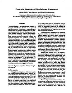


![[inria-00485915, v1] Delaunay Triangulation of ...](https://m.moam.info/img/260x300/inria-00485915-v1-delaunay-triangulation-of-_5b85cc58097c47b73c8b45fc.jpg)