delay estimation techniques working in the digital domain. First, it is eminently suitable to handle delays that are fractions of the sampling interval. This is in ...
Delay Estimation Using Adjustable Fractional Delay All-Pass Filters Mattias Olsson, Håkan Johansson, and Per L¨owenborg Link¨oping University, Div. of Electronic Systems, Dept. of Electrical Engineering, SE-581 83 Link¨oping, Sweden E-mail: {matol, hakanj, perl}@isy.liu.se ABSTRACT This paper presents a novel time-delay estimator utilizing an fractional-delay all-pass filter and Newton’s method. Solutions using a direct correlator and an average squared difference function are compared. Furthermore, an analysis of the effects of the batch length dependence is presented.
taken care of in a proper manner. The problem is now to find an estimate of the sub-sample difference d0 . In this paper we will look at two different basic principles for TDE. The first is the DC. The DC TDE estimator for a finite batch length N can be written as dbDC = min GDC (d) (3) d
1. INTRODUCTION
where
The need for time-delay estimation (TDE) between two signals arises in many different fields, including biomedicine, communications, geophysics, radar, and ultrasonics. In [1], a technique utilizing Farrow-based digital fractional-delay (FD) filters [2] was introduced for this purpose, filters with both amplitude and delay errors. In this paper we instead use all-pass FD filters with only delay error and lower filter orders [3] than their Farrow equivalents. The use of FD filters has two major advantages over other delay estimation techniques working in the digital domain. First, it is eminently suitable to handle delays that are fractions of the sampling interval. This is in contrast to methods that require additional interpolation [4]. Second, it can handle general bandlimited signals. This is in contrast to techniques that assume a known input signal, like a sinusoidal signal [5]. In general, two main basic principles for TDE have been used, Direct Correlation (DC) and Average Squared Difference Function (ASDF). In the literature it has been seen that ASDF has better performance for a finite batch length, although the DC principle can be shown to be ML (Maximum Likelihood). Using a single frequency signal (sinusoid) we will explain this phenomenon. Depending on the application, TDE can either be used in a batch-wise or a tracking fashion. In this paper we have assumed batch-wise operation, mainly because it simplifies the analysis. Following this introduction, Section 2 will provide a short introduction to TDE, followed by a presentation of the proposed delay-estimation technique in Section 3 and simulations in Section 4. Finally some conclusions are drawn.
GDC (d) =
N−1 1 X y(n, d)v(n) N n=0
(4)
and y(n, d) is a delayed version of x(n). It is shown in [6] that the DC principle is the Maximum-Likelihood (ML) TDE when noise is assumed to be Gaussian. However, since the observation time is finite the correlation can only be estimated. Another requirement is that the signals are optimally prefiltered. Another common basic TDE principle is ASDF. The ASDF TDE for a finite batch length N can be written as dbASDF = min FASDF (d) d
where
FASDF (d) =
N−1 1 X (y(n, d) − v(n))2 . N n=0
(5)
(6)
If we assume that the noise is uncorrelated and stationary and let N tend towards infinity, (4) and (6) become lim GDC = E{y(d)v} = Rvy (d)
(7)
lim FASDF = E {(y(d) − v)} = σ2y + σ2v − 2Rvy (d),
(8)
N→∞
and N→∞
Two (or more) discrete-time signals, originally coming from one source, might experience different delays. We model this as
where Rvy (d) is the correlation between v(n) and y(n, d). From these equations is seems like the two estimators are identical, except for the constant noise variances. However, this is not true, as can be seen in for example [7]. In simulations it is also seen that, when the noise becomes small, the DC algorithm reaches an error floor. This is due to the truncation of the estimation window, i.e. finite N. In Section 3 we give a more in-depth explanation of the effect of the limited window width.
x(n) = xa (nT ) + e1 v(n) = xa (nT − d0 T ) + e2
3. PROPOSED TIME-DELAY ESTIMATOR
2. TIME-DELAY ESTIMATION
(1) (2)
where d0 is the unknown sub-sample delay difference between the signals, T is the sampling period and φ is additive noise. It is assumed that e1 and e2 are uncorrelated with each other and with xa (t). Furthermore, we assume that the delay d0 is a fraction of T and that any integer sample delay has already been
To calculate y(n, d), the delayed version of x(n), a number of techniques can be used. The most straightforward is to use linear or higher order interpolation. This has problems though, since it is difficult to control the static delay error. In this paper we instead use adjustable fractional-delay all-pass filters.
3.1. Fractional Delay All-Pass Filters
d0
v(n)
-
The transfer function of a general all-pass filter of order M can be written as
(.)2
x(n) y(n,d)
FD
HA (z) =
z
−M
M X
−1
A(z ) where A(z) = 1 + am z−m . A(z) m=1
x(n)
(9)
am (d) =
C pm d p
m=1
(11)
Different methods exist to design the filter. In [9] a closed form technique to design all-pass filters with approximate linear phase is described. However, this method results in a filter order that is unnecessarily high. In this paper we have instead used a minimax ptimization approach described in [3], which gives a lower filter order. Let d˜ = τA (ω, d) − M + d be the delay error. The minimax solutions is then obtained by minimizing
(18)
The difference equation corresponding to the all-pass FD filter (9) is equal to y(n, d) = x(n − M) +
P X M X p=0 m=1
� � d p C pm x(n + m − M) − y(n − m, d) . (19)
The derivatives of (19) with respect to d needed for (15) and (16) are then calculated as y′ (n, d) =
y′′ (n, d) =
The minimization of (6) or the maximization of (4) can be done iteratively, for example using the well known Newton-Raphson algorithm, according to (14)
This algorithm converges very fast, typically three or four iterations are sufficient. Depending on the allowed implementation cost or time requirements we might also for example use a fixed value for the step-size (the inverse of the second derivative) or use an approximation of the second derivative (the Hessian) as in [4]. In Fig. 1 the principle of the proposed iterative estimator can be seen. The derivatives needed for (14) can be calculated analytically, for the ASDF approach, as (15)
and N−1 � � 2 X ′ y (n, d)2 + y(n, d) − v(n) y′′ (n, d) N n=0
N−1 1 X v(n)y′′ (n, d). N n=0
� p d p C pm (x(n + m − M)− d p=1 m=1 i y(n − m, d)) − C pm y′ (n − m, d)
P X M X
(20)
and
3.2. Iterative Estimation
′′ FASDF (d) =
G′′DC (d) =
(13)
over a range of ω and d.
N−1 2 X ′ (y(n, d) − v(n))y′ (n, d) (d) = FASDF N n=0
(17)
and
The phase delay response of the filter for a certain d can be written as ! PM 2 m=1 am (d) sin mω (12) τA (ω, d) = M − arctan PM ω 1 + m=1 am (d) cos mω
F ′ (dbn ) dbn+1 = dbn − F ′′ (dbn )
d 2/ d d 2
N−1 1 X v(n)y′ (n, d) N n=0
G′DC (d) =
p=0
˜