Change-point Problems. IMS Lecture Notes - Monograph Series (Volume 23, 1994). DESIGN OF CONTROL CHARTS. FOR DETECTING THE CHANGE POINT.
Change-point Problems IMS Lecture Notes - Monograph Series (Volume 23, 1994)
DESIGN O F C O N T R O L CHARTS FOR DETECTING THE CHANGE POINT BY YANHONG
WU
University of Toronto The discrete time change-point detecting problem is considered. The main purpose is to review some accurate approximations for the operating characteristics (ARLQ and ARL\) for three well-known detecting procedures: CUSUM, EWMA, and Shiryayev-Roberts procedures, based on the boundary correction technique. These approximations are shown to be very accurate compared with simulation and numerical values. The results can be used for the design of these control charts.
l Introduction. Suppose Xi,..., XΘ-I , XΘ-> ? Xn-> a r e a sequence of independent random variables, where Xι,..., X$-i are iid with the density a r e function /o(#), XQ, - 5-Xn? ϋd with the density function /i(#), and θ is the change-point and assumed to be unknown. The purpose is to find a detecting procedure in order to raise an alarm as soon as possible after the change occurs. The change-point problem has many applications in a variety of areas such as the surveillance of a system, monitoring the quality of production processes, and alarming for a flood etc.. For the convenience of discussion, we shall use the terminology from quality control. And for simplicity, we consider the normal case with /o following N(0,l), and f\ N(μ, 1) with μ > 0 unknown. Denote EQ[.] as the expectation when the change is at θ. In particular, EOQ and E\ denote the probability and expectation calculated when the change-point is at infinity and at the beginning, respectively. For a stopping rule r as the alarming time associated with a detecting procedure, two mostly used operating characteristics are the average in-control run length(AiZio) and the average out-of-control run length(Ai?JLi), defined by
AMS 1991 Subject Classification: Primary 62N10. Key words and phrases: Average run length, boundary correction, CUSUM, EWMA, Shiryayev-Roberts procedure.
Y. WU
331
and ARL\ are used to be evaluated by simulation as drawn by nomograms. Recent approaches are mostly through numerical methods such as the Markov chain method when the detecting process is Markovian, see Brook and Evans (1971) for the CUSUM procedure and Lucas and Saccucci (1990) for the EWMA procedure. The goal of this paper is to provide another simple method based on the boundary correction technique as discussed in Siegmund (1985) for the CUSUM procedure. The basic idea is to correct the control limit by adding the average overshoot at the alarming time. This method has several advantages. First, it has a clear relationship with the result in the continuous time case which usually has a simple close form. Second, it gives very simple formula which is extremely useful for the design purpose. Third, it has quite satisfactory accuracy for practical use. Three detecting procedures, i.e. CUSUM, EWMA and Shiryayev-Roberts procedures will be discussed. In Section 2, we first give the formulas for the approximations for ARUs when the control limit is large. The emphasis is for ARLo since it is crucial for the design. Comparisons with numerical values are made to show their accuracies. The main contribution of this paper is to give a simple design method for the EWMA procedure. In Section 3, we give some general guidelines on the practical use of these three procedures. Section 4 gives the technical details for the proofs of the related results in two subsections. First, we check the accuracy of the approximations for the ARL's in the CUSUM procedure. Then, we give the boundary correction results for the EWMA procedure. ARLQ
2. Approximation for ARVs. In this section, we give the approximations of ARL's for the three procedures and checking their accuracies by comparing with the numerical values. We begin with the CUSUM procedure. 2.1. CUSUM Procedure. When μ is unknown, we usually select a reference value δ to form a simple procedure. The CUSUM process for detecting the shift δ is defined by (1) where YQ is usually taken as 0. An alarm is made at T = min{n > 1 : Yn > d}. Siegmund (1985) gives the corrected diffusion approximations of ARL^s for the CUSUM procedure under the exponential family. In the normal case, AKLQ
«
332
DESIGN OF CONTROL CHARTS
as 6 -> 0, d -* oo, and id -+ constant, where /> = 0.583 for relatively small 6. Theorem 10.16 of Siegmund (1985) shows that the error of approximation (2) is on the order of o(l/δ). A careful reevaluation shows that the approximation is accurate in the order of o(l) as δ —• 0, see Section 4.1. The same conclusion is true for ARL\ where the approximation is given by ARL1(μ)
»
for μ > £/2. A more general discussion for the second order approximation for the ARVs of the CUSUM procedure can be seen in Pollak and Siegmund (1986). One may note that if we ignore the correction factor 2/>, (2) and (3) are the results for the continuous time CUSUM procedure (Taylor (1975)). Van Dobben de Bruyn (1968) uses several numerical methods to evaluate ARUs for the CUSUM procedure. Table 1 gives the comparison of the approximations (2) and (3) with the numerical values for δ < 1.2 and d = 2,2.5,3,4,5,6 respectively. We find that the relative error is within 2%. For large tf, higher order expansions for the mean overshoot will be necessary for a more accurate approximation, see Section 4.1 for the first order expansion. 2.2. Shiryayev-Roberts Procedure. The discrete time Shiryayev-Roberts procedure was first given by Roberts (1966). The procedure was formally discussed by Pollak and Siegmund (1985) in the continuous time case and shown to have similar behaviors as the CUSUM procedure. The ShiryayevRoberts process is defined as (4) with RQ = 0 for the chosen reference value δ. An alarm is made at r = inf{n > 0 : Rn > T}. The approximation for ARLo is given by Pollak (1987) for the exponentially family, from which, a simple approximation is given by ARLo « Tepδ,
(5)
where p is given as before. The accuracy of approximation (5) is even better than that for the CUSUM procedure. Table 2 gives the comparison with the simulated results for T = 100,300,500 respectively. The simulation is replicated 10,000 times. From the table, we see that for δ < 2.0, the approximation is very satisfactory.
Y. WU
333
For ARLι(μ), the approximation appears slightly complicated which is given by
ARL1(μ) = JT^-ΓΛ^T
+ Mn
see PoUak (1987). 2.3. EWMA Procedure. It is not difficult to derive the CUSUM and Shiryayev-Roberts procedures based on the likelihood principle and Bayesian approach, respectively. A more intuitive idea is to smooth the previous data in order to reduce the effect of noises in the sampling procedure. Two common methods are the moving average and the exponential smoothing (Roberts (1966)). The EWMA procedure based on the exponential smoothing has several quite interesting features. First, it gives the estimation of current mean, and thus can be used as a detecting process. Second, it is the optimal predicted value for the IMA(O,1,1) process which has been used for modeling the quality characteristic process for gradually increasing variation (Box and Jenkins (1963)). Third, it is Markovian and thus one can evaluated its operating characteristics quite easily (Lucas and Saccucci (1990)). Define the exponential smoothing of X\,..., Xn by
with ZQ = 0 and 0 < β < 1. The limiting variance of Zn can be easily found as
To detect a positive shift of mean, the usual EWMA procedure is defined to make an alarm at T = mi{n >l:Zn>B
= bσ^}.
From the definition of Z n , we see that after the change, the mean of Zn exponentially increases to the true mean δ. The design of EWMA procedure is rather complicated. In order to be able to detect the shift efficiently, a^b should be taken less that ί, and as small as possible in order to have small average delay time. However, b and β have to be chosen to satisfy the condition for ARLQ. Thus, there is an optimal design problem of choosing β and b which minimizes the average delay time for given ARLQ. In the continuous time case, Srivastava and Wu (1993) have considered this optimal design problem in terms of the stationary average delay time (Shiryayev (1963)). The main result shows that as ARL0 = T -> oo, in the
334
DESIGN OF CONTROL CHARTS
first order, the optimal smoothing parameter β* and control limit b* satisfies the following two equations: β = 2c*δ2/b*2,
(6)
1
4" Γ[Φ(x)Γ Hx)dx = T = ARL0,
(7)
P* Jo where c* = 0.5117. An approximation for β* can be obtained as 2
2
2
1 2
/Γ « 0.51176 /ln[0.40836 T(21n(0.4083ί T)) / ]
(8)
where obviously, the right hand side is required to be positive. Furthermore, it follows from (6) that as T —• oo, B =fcσoo« δ(/?/2)1/2 « 0.7156. This implies that the optimal control limit for Z n is approximately set at 0.715(5. Under this optimal design, for μ > 0.7156, we have
V V(l - 0.7156/μ)2 1)
+
°U* 2 J J '
see Section 4.2 for the exact results in the discrete time case. One can see that comparing to the CUSUM and Shiryayev-Roberts procedures, the approximation for the EWMA procedure is less accurate as the error is on the order of 1/lnT rather than lnT/Γ for the other two. Also when μ = ί, it is not difficult to check that the EWMA procedure is not as efficient as the other two procedures as the same ARLQ —> oo (Srivastava and Wu (1993)). The approximation (7) is too crude to be acceptable in the discrete time case. In Section 4.2, a more accurate approximation is obtained by adding the mean overshoot ER = E(ZT — δσoo) tofeσoo,which is roughly estimated as ER « β*p9
(9)
where p w 0.583 as before. By this correction, ARLo is about ARLo « e° 8 3 4 *Γ, in the first order, where T is given by (7), see Section 4.2. In order to detect a shift value 6 with ARL0 = Γ, the design for an EWMA procedure can be done in the following way. First, select a β based on
Y. WU
335
(8) with T replaced by Γe" 0 * 8 3 4 *. Then, let B = 0.715£ - 0.583/3. Although this does not give the ideal optimal design, it is quite good enough for practical use. An interesting method based on the Edgeworth expansion of the crossing probability is given by Robins and Ho (1978) by calculating the first four moments recursively. Table 3 gives some comparisons between the corrected diffusion approximation, the numerical values given in Robins and Ho (1978) , and the lower bound given by (16) of Section 4.2 which is the approximation by ignoring the overshoot. We see that the corrected boundary approximation gives much improved values than the lower bound. Ironically, the corrected diffusion approximation achieves its best accuracies around the region of {0.1 < β < 0.25}, which, according to Montgomery (1991), is the most desirable region for the value of β in practice. Table 1: Comparison of ARL0 and ARLX for CUSUM d 2.0
2.5
3.0
4.0
5.0
6.0
δ 0.0 0.4 0.8 1.2 0.0 0.4 0.8 1.2 0.0 0.4 0.8 1.2 0.0 0.4 0.8 1.2 0.0 0.4 0.8 0.0 0.4 0.8
ARL0 Num Approx 10.0 15.9 28.0 54 13.4 23.3 46.1 104 17.3 32.8 73.6 195 26.6 60.3 178 660 38.1 104 414 51.6 171 940
10.2 16.02 28.30 55.37 13.44 23.34 46.40 105.54 17.36 32.83 74.01 197.63 26.69 60.37 178.81 673.81 38.02 103.92 415.11 51.35 171.34 944.06
ARLt Num 10.0 6.86 5.06 3.96 13.4 8.73 6.24 4.79 17.3 10.7 7.44 5.62 26.6 14.9 9.88 7.28 38.1 19.4 12.4 51.6 24.0 14.9
Approx 10.2 6.85 5.04 3.92 13.44 8.71 6.21 4.74 17.36 10.69 7.40 5.56 26.69 14.91 9.84 7.22 38.02 19.39 12.31 51.35 24.04 14.80
*Numerical values are taken from Van Dobben de Bruyn (1968)
336
0.1 0.2 0.5 1.0 1.5 2.0
DESIGN OF CONTROL CHARTS
Table 2: Comparison of ARLQ for the Shiryayev-Roberts Procedure T = 300 T = 500 T = 100 Sim Approx Approx Sim Sim Approx 106.00 106.58 (0.49) 318.01 316.31 (1.99) 530.02 532.48 (3.74) 112.37 113.43 (0.77) 337.10 333.94 (2.74) 561.84 562.86 (4.87) 133.84 136.12 (1.23) 401.53 400.63 (3.83) 669.84 682.72 (6.46) 179.14 181.18 (1.75) 537.42 532.72 (5.12) 895.70 905.27 (8.97) 239.77 238.14 (2.39) 719.30 724.18 (7.16) 1198.84 1194.40 (12.0) 320.91 314.08 (3.17) 962.74 950.90 (9.46) 1604.57 1559.69 (15.62)
Table 3: Comparison of Approximations of ARLQ for EWMA procedure
0.05 2.0
2.25
2.50
2.75
3.0
3.5
4.0
LB Num. Approx LB Num. Approx. LB Num. Approx LB Num. Approx
LB Num. Approx LB Num. Approx LB Num. Approx
203.31 244.99 268.77 319.86 391.62 432.19 526.66 660.84 730.20 915.99 1183.63 1307.16 1694.79 2242.04 2493.02 7103.38 9136.09 11090.78 39349.64 45821.86 64773.33
0.10 98.98 149.15 142.85 155.72 244.62 230.10 256.40 424.14 450.25 445.94 778.81 833.96 825.09 1504.96 1651.16 3458.18 6582.11 6017.31 19156.82 37821.50 34875.90
0.25
36.25 80.51 74.28 57.03 137.32 125.86 93.90 248.42 226.21 163.32 477.26 433.75 302.18 974.68 890.44 1266.52 4936.30 4627.41 7015.98 33197.59 31729.11
*LB: Lower bound; Num: Robins and Ho (1978); Approx: corrected boundary approx.
Y. WU
337
3. General Discussion. (l)In the above section, we emphasized the approximations for ARLo since it is critical for the design of these control charts. The traditional approximation by ignoring the overshoot significantly underestimates the true value as we can see from Tables 1-3. The approximation of ARLi is also important if we want to compare these three procedures and to consider the economic design. The comparisons among the three procedures have been done by many authors by a variety of methods. Roberts (1966) compared several charts by simulation. The currently most used method in quality control literature is the Markov chain method, see Lucas and Saccucci (1990) for the comparison between the CUSUM procedure and the EWMA procedure. This method is obviously very space-consuming. The theoretical comparisons have been done by Pollak and Siegmund (1985) and Srivastava and Wu (1993) under the continuous time model. A more recent study by Pollak and Siegmund (1991) also considered the case when the initial level is unknown. (2) Only comparing ARL\ may be misleading as it considers only the case when the change occurs at the beginning. A typical example is the FIR (fast initial response ) technique, and also see Srivastava and Wu (1993) for an example in the one-sided EWMA procedure. Thus, more reasonable measures for the average delay time should be chosen. Three interesting ones are the conditional stationary average delay time, the unconditional stationary average delay time and the maximum conditional delay time (Pollak and Siegmund (1985), Shiryayev (1963), and Lorden (1971)). The CUSUM procedure is optimal in the worst case and the Shiryayev-Roberts procedure is optimal in the stationary case. The asymptotic behaviors of the conditional and the unconditional stationary delay time are almost same as ARLo is large. The comparisons among these three procedures can be seen in the literature mentioned above. (4) In this note, we only considered the one-sided shift case. The twosided shift case can be similarly discussed (Siegmund (1985), Pollak and Siegmund (1991), Lucas and Saccucci (1990)). A theoretical treatment for the two-sided as well as the multivariate EWMA procedures will be discussed in another communication. 4. Technical Results. In this section, we give some technical details for the results given in Section 2. The readers are assumed to be familiar with Wald's likelihood identity and Stone's strong renewal theorem. We refer to Siegmund (1985) for a more detailed discussion. We have two objectives. One is to show that the approximations given in (2) and (3) are accurate in the second order of δ under appropriate conditions. The other is to give a heuristic argument for the approximation of ARLQ for the EWMA procedures by using
338
DESIGN OF CONTROL CHARTS
the boundary correction technique. 4.1. Error Checking for the Approximations (2) and (3). We only give the details for ARLQ. For ARL\ as well as the stationary average delay time, Pollak and Siegmund (1986) have given a more general discussion in the exponential family. Define N = inf{n > 0 : Sn < 0 or > d}, and τd = inf{n > 0 : Sn > d}, and r_ ( + ) = inf{n > 0 : Sn < (>)0}. Then
EoN Po(SN>d)
ΔΏT
E0SN -δ/2P0(SN>dy
The key to guarantee the accuracy of the following approximations is the strong renewal theorem which states that as d —• oo, uniformly for δ > 0 and y>o, \Pi(STd
-d>y)~
P1(R
> y)\ - o ( e " ^ ) ,
for a positive constant r, where Pι(R G dy) = P\(ST+ > y)/EιSr+dy, see Siegmund (1979) and some refined result by Lotov (1991). LEMMA 1.
Pχ(SN The proof can be obtained similar to Lemma 4. LEMMA 2.
P^r.
= oo)/Eo(Sτ_) =
-δEie-SR.
LEMMA 3. rd
E0SN = EO(ST_) + ErfPoiSN > d)(l + o(e--rd)) + E0(SN; SN > d). PROOF.
Note that E0SN = E0(SN; SN < 0) + E0(SN; SN > d).
339
Y. WU On the other hand, EO(ST_) = EO(ST_;SN = E0(SN
< 0) + EO(ST_;SN
SN < 0) + Eo[Eo[Sτ_ ; 5 N < 0) + E1RP0(SN
> d) \SN]\SN>d] > d)(l + o(e" r < ί )).
Based on Lemmas 1-3, we get
^)-iPa(r_ = oo) E0(SN\SN
> d)](l +
o(e-rd))
•o(e-rd)).
The only remaining thing is to evaluate EQ(SN\SN
> d). This is given by
LEMMA 4. Ji/QyoN\oN > d) = α H———_^p (^1 + oye
)).
PROOF. By noting that
E0(STd -d;τdd)
+ E0(STd -d;τd
d) =• 1
- d)e-ss^\SN};
SN < 0]
δd
* - e- EQ[ExRe-δReSSN;SN = e-SdE1Re-δRP1(SN
< 0])(l + o(e~rd))
d
where Lemma 1 is used in the last step. Finally, we have THEOREM 1. As d —• oo,
e
d
>
340
DESIGN OF CONTROL CHARTS
By using Holder inequality and the fact that (Eλe-δR)-χ we get
EλRe~δR
^""'-•-'^^M.-')
> EXR,
do)
As δ is small, we may replace E\R by p when the drift is taken as zero, which gives us (2). Thus, (2) slightly overestimates the true ARLo, which is also confirmed from Table 1. A similar argument shows that (3) slightly underestimates the true ARL\. In the following, we shall show that (2) is actually accurate in the order of o(l) as δ —» 0 and d —> oo such that δd remains bounded. By taking Taylor series expansion, it follows that Eλe-δR
= 1 - δExR + ^EτR2
+ o(δ2).
(11)
A result from Problem 10.2 of Siegmund (1985) gives that EιR = p+δ-(p2-p2)
+ o(δ),
(12)
where p2 = E\R2. Substituting (12) into (11) and simplifying it, we get Eλe-SR
= e-sp(l
+ o(δ2)).
(13)
On the other hand,
(Ihe-MyiEiRe-*11
= EΎR - δ{ErR2 - (E^R)2) + o{6)
= P- \{P2 - P2) + o(δ). Combining with (12), we get 811
EtR + (Exe-s^ExRe-
= 2p + o(δ).
(14)
Substituting (13) and (14) into (10), we see that the approximation (2) is actually accurate up to order o(l), which slightly improves Theorem 10.16 of Siegmund (1985) and also confirms accuracy of the approximation. The above argument can be easily adapted to the exponential family case. In the nonsymmetric case, the second order approximations involve the third moment of i2, see Pollak and Siegmund (1986) for some specific results. When 6 is too large, even this second order approximation may not be satisfactory. In this case, we should use the result of Theorem 1 and take more terms in the expansion for E\R in δ. 4.2. Boundary Correction for EWMA Procedure. In this subsection, we discuss in detail the approximations for the EWMA procedure. The key is to form a martingale for the EWMA process Zn which only involves Zn and the
Y. WU
341
time n. We write B = δσoo as the control limit for the EWMA process. The following lemma is the key for our discussion. n
1
Denote φ(u) = Σ£° c((l — β) ~ βu) as the cumulant generating function for ZQO, where c(u) is the cumulant generating function for Xχm From Novikov (1990), it is known that LEMMA 5.
Yn = Γ
uZ
i(e » - l)e-+Mdu + nln(l - β)
is a martingale. In the normal case,
when the mean is μ after the change. By changing the order of integrals, we have i fZrn&rt* ARLo = _ln(1_β)E Jo [ _Hl_β)
j\φ(χ)ΓιΦ(x)dχ,
(16)
which is similar to (7) in the continuous time case by simply changing -ln(l β) to β. As we showed in Table 3, this lower bound is too crude for practical use. We thus consider the effect of the overshoot. Similar to the random walk case, we define the following ladder variables based on the EWMA process Zn\ TW = inf{n > 0 : Zn > 0}, τ& = inf{n > 0 : Z n + τ ( 1 ) > Z τ ( 1 ) }, generally, τW = inf{n > 0 :
342
DESIGN OF CONTROL CHARTS
Thus, r = rW +
+ r W with N =i
By writing ^n
=
we see that Zn and Z n are distributionally equivalent. If we approximate Zτ(i)+...+r(N-i) by B, then the mean overshoot can be approximated by E[Zr-B]&E[Zv-(l-(l-βγ)B], where v = min{n > 0 : Zn > (1 - (1 - β)n)B}. Thus, the calculation of the mean overshoot is transformed into another boundary crossing problem with a curved boundary. In the following, we look at the mean overshoot behavior as β -+ 0 as required under the optimal design. As β —> 0, Zn/β behaves like a random walk with drift 0, and on the other hand, (1 - ( 1 -β)n)/β
-n.
Locally speaking, the ladder variables for the EWMA process can be approximated as a sequence of boundary crossing times for a random walk with randomly increasing drift parameters. Thus, a better approximation can be obtained as ER « βρ(-B) as β -> 0, where ρ(-B) = ES*+/2EST+ is evaluated with mean -B. As δ -> 0, p(-J5) -* p = 0.583. The numerical comparison with the numerical values given in Table 3 shows that this approximation is generally good. For example, for β = 0.10 and b = 2.0, the corrected diffusion approximation gives 149 which is very close to the numerical value 143 given by Robins and Ho (1978). To see how much effect of this overshoot on ARLQ, we consider the first order approximation as 6 -> oo. Under the optimal design, recall that b(β/(2/ • 0.715£. Based on this, the following rough approximation can be
Y. WU
343
obtained. 1 A R L o
=
-\n(l-β)E [φ(x)]-1Φ(x)dx
- β)E / Jo
as £ is small. Therefore, in the first order, the correction factor for the EWMA procedure lies between the correction factors of CUSUM and Shiryayev-Roberts procedures. Similar to the other two procedures, this correction may become less satisfactory when B = bσoo becomes larger. A more accurate approximation can be obtained by taking the second order expansion for p(μ) in μ. Partial results have been given by Chang (1989). For example,
EμSτ+ = -±=(l + μp+£p2
+ o(μ>)).
Finally, we point out that the above argument is only heuristic, a formal treatment can be done similar to the method used by Pollak (1987) by considering the behaviour of Zn in the region (B(l — β),5) with a properly chosen small 6. More specifically, let rB-t
= inf{n >0;Zn>
B(l - e)}.
Γ
Consider the process {^τBn_c)+n} f° n > 1. Then it will either cross the boundary B soon, or "not at all" in a near future. If it does, then locally, it behaves like a random walk; if it doesn't, wait until next time it crosses B — e again. Details will be presented somewhere else. A different approach may be to use the method of Siegmund (1985, Chap. 4) based on the time-scale transformation. Acknowledgement: I am grateful to the referee for many helpful suggestions. This research is partially supported by a Postdoctoral Fellowship from NSERC.
344
DESIGN OF CONTROL CHARTS
REFERENCES Box, G. E. P and JENKINS, G. M. (1963). Further contributions to adaptive quality control: simultaneous estimation of dynamics: Non-zero costs. Bull. Internet. Statist. Inst. 34, 943-974. D. and EVANS, D. A. (1971). An approach to the probability distribution of CUSUM lengths. Biometrika, 59 539-549.
BROOK,
T. (1989). Random Walks, Moderate Deviations, and the CUSUM Procedure, Ph.D. dissertation, Stanford University.
CHANG,
VAN DOBBEN DE BRUYN,
C. S. (1968). Cumulative Sum Tests. Griffin, London.
G. (1971). Procedures for reacting to a change in distribution. Ann. Math. Statist. 42, 1897-1908.
LORDEN,
V. I. (1991). On random walks in a strip. Theory Prob. Appl. 36, 165-170.
LOTOV,
J. M. and SACCUCCI, M. S. (1990). Exponentially weighted moving average control schemes: properties and enhancements. Technometrics, 32, 1-29.
LUCAS,
D. C. (1991). Introduction to Statistical Quality Control. 2nd ed., John Wiley and Sons, New York.
MONTGOMERY,
A. (1990). On the first passage time of an autoregressive process over a level and an application to a "disorder" problem. Theory Prob. Appl. 35, 269-279.
NOVIKOV,
PAGE,
E. S. (1954). Continuous inspection schemes. Biometrika, 41, 100-114.
M. (1987) Average run lengths of an optimal method of detecting a change in distribution. Ann. Statist., 15, 749-779.
POLLAK,
M. and SIEGMUND, D. (1985). A diffusion process and its applications to detecting a change in the drift of Brownian motion. Biometrika, 72, 26780.
POLLAK,
M. and SIEGMUND, D. (1986). Approximations to the ARL of CUSUM tests. Technical Report, Department of Statistics, Stanford University.
POLLAK,
M. and SIEGMUND, D. (1991). Sequential detection of a change in a normal mean when the initial value is unknown. Ann. Statist., 19, 394-416.
POLLAK,
S. W. (1959). Control chart tests based on geometric moving average. Technometrics, 1, 239-250.
ROBERTS,
S. W. (1966). A comparison of some control chart procedures. Technometrics, 8, 411-430.
ROBERTS,
Y. WU
345
P. B. and Ho, T. Y. (1978). Average run length of geometric moving average charts by numerical methods. Technometrics, 10, 85-93.
ROBINS,
A. N. (1963). On optimum methods in quickest detection problems. Theory Prob. AppL 13, 22-46.
SHIRYAYEV,
D. (1979). Corrected diffusion approximations in certain random walk problems. Adv. AppL Prob. 11, 701-719.
SIEGMUND,
D. (1985). Sequential Analysis: Tests and Confidence Intervals. Springer, Berlin.
SIEGMUND,
M. S. and YANHONG WU (1993). Comparison of EWMA, CUSUM and Shiryayev-Roberts procedures for detecting a shift in the mean. (To appear in Ann. Statist. )
SRIVASTAVA,
H. M. (1975). A stopped Brownian motion formula. Ann. Prob., 3, 234-246.
TAYLOR,
Wu, YANHONG (1991). Some Contributions to On-line Quality Control. Thesis, University of Toronto. DEPARTMENT OF STATISTICS UNIVERSITY OF TORONTO TORONTO, ONTARIO, CANADA M5S
1A1
Ph.D.