Abstract— This correspondence deals with the segmentation of a video clip into independently moving visual objects. This is an important step in structuring ...
1
Detection of moving objects in video using a robust motion similarity measure Hieu T. Nguyen,
Marcel Worring,
Abstract— This correspondence deals with the segmentation of a video clip into independently moving visual objects. This is an important step in structuring video data for storage in digital libraries. The method follows a bottom-up approach. The major contribution is a new well founded measure for motion similarity leading to a robust method for merging regions. The improvements with respect to existing methods have been confirmed by experimental results. Keywords— motion similarity, motion segmentation, content-based indexing, video analysis
I. I NTRODUCTION Video is becoming an important datatype in digital libraries. Besides the traditional verbal user queries, the library should support queries based on object shape and motion. Objects and their characteristics therefore form basic units for content-based retrieval and presentation of video. They are further useful for video compression and the creation of hypervideo documents. Our correspondence deals with motion segmentation, i.e. the decomposition of a video scene into independently moving visual objects. Starting from an oversegmentation of the scene, it merges regions based on motion similarity. The paper is structured as follows. In Section II we formulate the problem and provide a short review of existing literature. Our new region merging method is described in Section III. Section IV shows the results of applying the method on some standard test image sequences. II. P ROBLEM
FORMULATION
Suppose there are K moving rigid objects in the scene, we want to recover their regions of projection C1 , ..., CK on the image plane. When a surface of a rigid moving object is planar or distant enough from the camera, its optic flow at position x = (x, y) is well modeled by the quadratic transformation [1]: vx vy
= =
a1 + a2 x + a3 y + a7 xy + a8 x2 a4 + a5 x + a6 y + a7 y2 + a8 xy
(1)
where ϑ = (a1 , . . . , a8) are the motion parameters of the moving surface. In existing literature the modelling of the optic flow of a region by a parametric model is used either in the direct form (1) or in combination with the intensity matching equation. In both cases we can consider it in the generalized form: y(x) = f(x; ϑk ) + εx
∀x ∈ Ck ;
k = 1, ..., K
(2)
where y(x) is the measurement at pixel x. In (1) y would correspond to the vector (vx , vy ). f is a known function. ϑk is the vector of motion parameters of region Ck which is unknown a The authors are with the Intelligent Sensory Information Systems group, University of Amsterdam, Faculty of WINS, Kruislaan 403, NL-1098 SJ, Amsterdam, The Netherlands. Email: { tat,worring,anuj }@wins.uva.nl
and Anuj Dev
priori and is to be estimated together with Ck . The term εx represents the measurement error. The problem can then be viewed as segmenting the data, which are described by multiple regression models, into groups so that data in each group is described by a common model. The challenge is that both Ck and ϑk are not known a priori. First, a granularity level for regions has to be selected. Pixelwise classification is inherently not reliable due to the aperture problem as pixels in homogeneous regions can be assigned to any model. Trying to overcome this problem recent methods start from homogeneous regions, usually obtained through intensity or color segmentation. Then regions are merged according to motion based criteria. Several criteria have been proposed [1], [8], [5], [2]. The earliest method [8] used a scaled Euclidean distance. This measure has been criticized to be sensitive to inaccuracy in parameter estimation as well as the choice of the scaling matrix [5], [2]. Furthermore, we have shown that the merging results depend on the choice of the origin of the coordinate system [6]. In [9] the merging decision is based on whether residuals in two regions can be expressed by one Gaussian distribution. We found that the measure tests for the difference in motion parameters of the regions as well as difference in noise variance. The latter test is, in fact, not needed. Altunbasak et al [2] proposed a merging procedure minimizing the residual over all regions. The global minimum corresponds to the maximum likelihood solution for both region labels and motion parameters. The problem is that the objective function usually has very many minima and the proposed technique finds a local minimum only. A good starting point is therefore required. An elaborate method was developed by Moscheni et al [5]. However, an asymmetric similarity measure is used. Moreover, the method depends on a large number of parameters that need to be set. In conclusion, existing merging criteria are still ad-hoc. To this end, we propose a new rigorous approach for definition of motion similarity and develop a new merging method utilizing the strengths of the methods of [9] and [2] and at the same time overcoming their shortcomings. III. N EW
ROBUST METHOD FOR REGION MERGING .
A. Motion statistics based region similarity Let R1, ..., RM be the regions obtained from the initial oversegmentation. We assume that the initial segmentation is such that there are no regions occluding the object boundaries, hence, each Ri is a subregion of one Ck . Let θ i be the vector of motion parameters of Ri, then θi ∈ {ϑ1 , ..., ϑK }. Obviously, two regions undergo a common motion and therefore are supposed to be merged if and only if θ i = θj . In practice, however, we have ˆ i of θ i which is commonly to base our decision on an estimate θ
2
where
obtained via least squares minimization: X
ˆ i = arg min Si (θ) where Si (θ) = θ |y(x) − f(x; θ)|2 θ x∈Ri (3) In the presented method we first apply the robust estimation technique given in [4] to detect outliers defined as pixels whose measurement is not described by the same model as the majority of pixels in the region. Then the parameters are reestimated for the clean data using least-square. Although the influence of the ˆ may be different from the true θ due to outliers is reduced, θ noise. As a consequence, two regions of the same object may turn out to have different estimated motion parameters. Therefore, inference about the equality of θ i and θ j should be made by means of a statistical test. We need to test the hypothesis : H0 : θ i = θ j versus H1 : θ i 6= θ j
(4)
The problem is much like testing whether two sets of data y
Sˆi = min Si (θ) θ
∆(i, j)
ˆ ij = (Hi + Hj )−1 (Hi θ ˆ i + Hj θ ˆj ) θ
Fig. 1. Test if two sets of data points represent the same model.
points represent the same line ( see Figure 1). Let L be the likelihood function of the measurements in Ri and Rj , given θ i and θ j : L(y(x), x ∈ Ri ∪ Rj |θi , θj ) = (2πσi2 )−ni /2(2πσj2 )−nj /2 × 1 1 exp{−[ 2 Si (θ i ) + 2 Sj (θ j )]} 2σi 2σj (5) where σi and ni are the variance of the measurement errors and the number of pixels in Ri respectively. We construct the loglikelihood ratio statistic: (6)
If ∆ exceeds a given threshold T , H0 is rejected in favor of H1. It is easy to show that: Si (θ) Sj (θ) Si (θ) Sj (θ) ∆ = min[ 2 + ] − min 2 − min σi σj2 σj2 θ θ σi θ
(7)
Although in practice noise variance may show minor variation over the image, it is advantageous to assume it is constant over the whole image. That means σi = σj = σ. Then ∆=
1 ˆ [Sij − Sˆi − Sˆj ] σ2
1 ˆ ˆj )> Hi (Hi + Hj )−1 Hj (θ ˆi − θ ˆj ) (θ i − θ 2σ2 1 ˆ ˆj )> [H−1 + H−1 ]−1(θ ˆi − θ ˆ j ) (9) (θ i − θ i j 2σ2
where Hi is the hessian matrix of Si (θ), which is constant if f is linear. This matrix is a by-product of minimization of Si (θ). It is important to note that 2σ 2 H−1 is the covariance matrix of i ˆ i. Moreover, when a merging decision is accepted, the optimal θ motion parameters and the hessian of the union Ri ∪ Rj can be obtained directly from those of Ri and Rj as follows [6]:
x
∆(i, j) = −2 log( sup L/ sup L) θ i =θ j θ i 6=θ j
= =
θ2
R2
Sˆij = min[Si (θ) + Sj (θ)] θ
Hence, ∆ is proportional to the increase in the residual sum of squares when a common model is chosen for the two regions instead of the optimal model for each one. This statistic yields our measure for similarity between motions of two regions Ri and Rj . As an aside if we test the hypothesis: H0 : θi = θ j AND σi = σj versus H1 : θ i 6= θj OR σi 6= σj we then get the statistic used in [9]: Λ = nij log(Sˆij /nij ) − ni log(Sˆi /ni ) − nj log(Sˆj /nj ). The drawback of Λ is that it is non-zero even if the motion parameters estimated in the two regions are equal. For simplicity we now focus on the case where f is linear with respect to θ. If not, all results below are applicable if Taylor’s approximations of f are made. We have shown that [6]:
θ1
R1
and
(8)
Hij = Hi + Hj (10) We also want to assess how close the motion of Ri is to a hypothesized motion model with parameters ϑ. In this case ϑ is deterministic and its covariances are zero, eq. (9) then becomes: ˆi , ϑ) = ∆1 ( θ
and
1 ˆ ˆ i − ϑ) (θ i − ϑ)> Hi (θ 2σ2
(11)
This expression coincides with the Mahalanobis distance beˆ i and the class center ϑ. tween θ B. Properties of the proposed measure −1 It is important to note that 2σ1 2 [(H−1 + H−1 in (9), the i j )] ˆ ˆ j , is the inverse of the covariance matrix of the vector θ i − θ optimal scaling matrix. This contrasts the ad-hoc one used in [8]. The other desirable properties of ∆ are given in the following theorem, proofs of which can be found in [6]: Theorem 1: The similarity measure ∆(i, j) defined in (9) satisfies the following properties: 1. ∆(i, j) > 0; ∆(i, i) = 0; ∆(i, j) = ∆(j, i) 2. ∆ has a chi-squared distribution χ2p (λ) with degree of freedom p equal to the number of the motion parameters, whose non-centrality parameter is:
λ=
1 (θ i − θj )> Hi (Hi + Hj )−1 Hj (θ i − θj ) 4σ2
(12)
3. For the velocity model (1) ∆ is invariant to affine transformations of the coordinates in the image space.
3
The second property guarantees that ∆ well discriminates regions undergoing the same motion from those undergoing different motions. In the former case θ i = θj and, hence, λ = 0 and ∆ has a central chi-squared distribution. In the latter case λ > 0, the distribution of ∆ becomes non-central and the measure tends to be large as the chance it exceeds the threshold T is much higher. The third property guarantees the independence of the merging result from translation or rotation of the coordinate system which is not the case for some earlier methods [8]. The proposed measure is not a metric as required by many standard clustering methods. It satisfies the conditions of positivity and symmetry as shown above, but not the triangular inequality. Thus, ∆ is a good measure when an appropriate merging method is developed. C. Merging procedure Maximum likelihood approach for merging regions requires minimization of the residual sum of squares over all regions: S(z, ϑ1 , . . ., ϑK ) =
M X
Si (ϑzi ) =
i=1
M X X i=1
|y(x)−f(x; ϑzi )|2
x∈Ri
(13) where z = (z1 , .., zM ) and zi ∈ {1, . . ., K} is the region label specifying the index of the global moving surface to which R i belongs. A similar approach was used in [2]. We now show that the above minimization can be viewed as a generalized version of standard K-means clustering and the algorithm used in [2] can be improved to save computations. Considering f is linear with respect to the motion parameters and applying Taylor’s theorem, it is easy to show that: 1 ˆ > ˆ Si (ϑzi ) = Sˆi + (θ i − ϑ zi ) H i (θ i − ϑ zi ) 2
(14)
Since Sˆi is constant, the minimization of S boils down to minimization of S0 where: 1X ˆ ˆ i − ϑz ) (θ i − ϑzi )> Hi (θ i 2 M
S0(z, ϑ1 , .., ϑK )
=
i=1
=
σ
2
M X
MERGING STAGE 2 1. Assign each θˆi to the nearest cluster center ϑzi , using the distance measure ∆1, defined in (11). 2. Update the cluster centers ϑk so that the sum of differences between the center and the cluster members is minimized. As we showed in [6] the new ϑk can be found by solving the following system of equations: X X ˆi ( Hi )ϑk = Hi θ (16) zi =k
zi =k
3. Repeat 1 and 2 until cluster membership is unchanged. Since the number of objects is specified in the beginning, the value of variance of noise does not affect the final result and we do not have to specify σ. The convergence in the second stage is guaranteed as the cost function always decreases. Actually, if starting from the same initial set of cluster centers, the second stage gives the same result as the two-step iterative procedure used in [2] does 1 . However, our algorithm requires much less ˆ i and Hi are already obtained computations, considering that θ from the least-squares minimization of Si . Note also, that the above algorithm merges non-adjacent regions as well, which is not the case for some methods [1], [9], [5]. IV. R ESULTS In Figures 2 and 3 we show the results of applying the proposed merging algorithm on standard test sequences. The initial segmentation was obtained with the morphological multiscale technique [7]. The results for Table Tennis and Flower Garden were obtained with optic flow matching. As measurements y(x) we used the dense optic flow field, computed from two successive images using the hierarchical method in [3]. For the Calendar sequence we used the model, which is based on the linearized intensity matching equation [6]. The improvements due to the use of the new similarity measure are confirmed by comparison with Figure 2c,d, in which we show the results of the existing methods in [9] and [2] applied for the same set of initial regions. More elaborate evaluation can be found in [6]. V. C ONCLUSION
ˆi , ϑz ) ∆1 ( θ i
(15)
i=1
This is, in fact, similar to the objective function in the K-means ˆ i and algorithm except that the Euclidean distance between θ ϑzi is replaced with the Mahalanobis distance (11). Like traditional K-means, good initial cluster centers are required. The ad-hoc pixel-based technique used in [2] for deriving the initial set of global motions is very likely to miss the motion of foreground objects. We propose an algorithm encompassing two stages where the first one performs hierarchical region merging and provides a good starting point for the generalized K-means iterative procedure in the second: MERGING STAGE 1 1. Specify K, the number of objects. Initialize each cluster with one region: Cm = {Rm }; m = 1, ..., M . 2. Merge the two adjacent clusters Ci and Cj with the smallest ∆ defined in (9). Repeat until the number of clusters is reduced to K.
We have proposed a new criterion for similarity of regions movement in a video scene based on a statistical test for equality of motion parameters. The uncertainty in parameter estimation is incorporated in an optimal way. Using this measure we have developed a new merging algorithm consisting of two stages. The agglomerative merging in the first stage provides a good starting point for the second stage in which the regions are merged according to a K-means like algorithm. The improved performance over existing methods has been demonstrated on real sequences. As extracted objects and their motion parameters are accurate, they can be used for content-based video retrieval in digital libraries. R EFERENCES [1] G. Adiv, “Determining 3d motion and structure from optical flows generated by several moving objects,” IEEE Trans. on PAMI, vol. 7, no. 4, pp. 384–401, 1985. 1 We note, by the way, that in [2, section 4.3] the mixed use of intensity matching and optic flow matching dose not guarantee convergence.
4
a)
b)
c)
d)
Fig. 2. a) One frame from Table Tennis and the initial segmentation, consisting of 23 regions; b) Merging result of the proposed method, K=4; c) Result of the method in [9]; d) Result of the method in [2].
a)
b)
Fig. 3. Merging result of the proposed method for a) Flower Garden, K=3; and b) Calendar, K=5. Object boundaries are marked by white lines.
[2] Y. Altunbasak, P.E. Eren, and A.M. Tekalp, “Region-based parametric motion segmentation using color information,” Graphical Models and Image Proc., vol. 60, no. 1, pp. 13–23, Jan. 1998. [3] J.R. Bergen, P. Anandan, K.J. Hanna, and R. Hingorani, “Hierarchical model-based motion estimation,” in Proc. 2nd European Conf. of Comp. Vision, 1992, pp. 237–252. [4] P.J. Huber, Robust statistic, John Wiley, New York, 1981. [5] F. Moscheni, S. Bhattacharjee, and M. Kunt, “Spatiotemporal segmentation based on region merging,” IEEE Trans. on PAMI, vol. 20, no. 9, pp. 897– 915, Sept. 1998. [6] H.T. Nguyen, M. Worring, and A. Dev, “Robust motion-based segmentation in video sequences,” Tech. Rep. 4, Intell. Sensory Inf. Sys. Group, Univ. of Amsterdam, Dec. 1998, available at http://carol.wins.uva.nl/˜rein/isis.html. [7] P.Salembier, “Morphological multiscale segmentation for image coding,” Signal Processing, vol. 38, no. 3, pp. 359–386, Sept. 1994. [8] J.Y.A. Wang and E.H. Adelson, “Representing moving images with layers,” IEEE Trans. on Image Proc., vol. 3, no. 5, pp. 625–628, Sept. 1994. [9] L. Wu, J. Benois-Pineau, Ph. Delagnes, and D. Barba, “Spatio - temporal segmentation of image sequences for object-oriented low bit-rate image coding,” Signal Proc. : Image Comm., vol. 8, pp. 513–543, Sept. 1996.