Many of those students feel that learning mathematics â at least to the extent that it is usually .... students a deep understanding of numerical analysis and therefore do not contain the technical .... cessing â blurring, deblurring and embossing:.
DEVELOPMENT AND IMPLEMENTATION OF APPLICATION-BASED EXERCISES FOR THE MATHEMATICS EDUCATION OF ENGINEERS M. Plaue, M. Scherfner ¨ Berlin (GERMANY) Technische Universitat {plaue, scherfner}@math.tu-berlin.de
Abstract In mathematics courses for engineers, student motivation frequently suffers from the lack of a clear connection of the purely mathematical subjects to topics that the students feel are more relevant for their specific field of study. One method to establish such a connection is the additional employment of application-driven exercises. In this paper, we describe the development of such exercises and their ¨ Berlin, implementation with the courses Analysis I and II for engineers held at the Technische Universitat Germany. One particular novelty of the problem sheets we developed, compared to commonly available applicationbased problem collections, is the fact that they are especially designed so that the mathematical content parallels the regular curriculum of the course. Very similar to a student project, each set of exercises examines one basic topic in engineering or natural science with particular emphasis on mathematical problem solving. Each student chooses a project at the beginning of the semester which is then worked on collaboratively in small groups during the whole term. In total, we developed 13 problem sheets that aim at covering the scope of at least 14 different fields of engineering as well as computer science while conveying the skills and knowledge necessary for successfully completing the mathematics course. As particular examples, we will discuss two of the projects in more detail, namely on the subjects of the tractrix (limits and differentiability) and image processing (partial differential equations). The latter was particularly designed for students of computer science to show them that some inherently discrete problems they will be confronted with, like the processing of digital images, may be efficiently modeled with the continuous methods of mathematical analysis. In this project, the students make extensive use of the numerical computing software MATLAB. Finally, we will present the results of a student evaluation showing a generally positive reaction to the new curriculum. Keywords: mathematics education for engineers, application-based exercises
1 INTRODUCTION In most universities, the mathematics education of engineering students is separately organized from their applied courses. There are a number of immediate practical reasons why this is not done differently, some of which are: • The mathematical content is extensive and mostly self-contained; • introducing a new mathematical concept or tool each time it arises with an applied problem is cumbersome and would lead to topically fragmented courses and confusion among students; • students of different branches of engineering need to learn – more or less – the same mathematical topics; • it would be more difficult to assess if a particular student has learning problems with the mathematical content or the specific concepts of her or his main field of study. However, a major disadvantage of this approach are the motivational problems teaching assistants and lecturers of mathematics courses frequently experience with first-year students of engineering (or physics). Many of those students feel that learning mathematics – at least to the extent that it is usually taught – is detached and of lesser importance to their particular field of study. Considering the fact that many applications of the more complex mathematical concepts arise only in topics covered by courses
of later semesters, they cannot be blamed for this assessment. One way to overcome these motivational problems is the implementation of application-based exercises ¨ (TU) Berlin – where mathematics is taught with the mathematics courses. At the Technische Universitat to engineers from more than 14 different fields – we designed problem sheets each of which covers a basic topic of natural science or engineering. The exercises included with these problem sets convey the mathematical content of the courses Analysis 1 and 2 for engineers where they were successfully integrated. At the beginning of the semester, each student chose a problem set she or he wishes to work on together with two fellow students. It should be noted that while there are many collections of application-driven math exercises available (for example, [4]) we designed our problem sets specifically to parallel the curriculum of said courses. In the following section, we will give a general description of our problem sheet design and present two of the sheets in more detail. The implementation of these problem sheets should not lead to less time for teaching the mathematical content, and it is imperative to minimize the additional workload for the teaching staff and the students. In Section 3, we will describe how we accomplished this. In Section 4, we will shortly present a student evalution and conclude with Section 5, giving some final remarks and practical hints.
2 EXERCISES In order to help each student with choosing the problem sheet that suits her or his particular interests best, each problem set is preceded by a detailed introduction in which the main applied topics and scope is illustrated. Since the necessary background for understanding the more technical content would still have to be conveyed during the course, mathematical explanations are kept to a minimum at this point. However, a short list of mathematical topics is included for the sake of completeness. More importantly, we included a list of fields of engineering for which the respective application may be regarded as most important. The actual exercises of each problem sheet are divided into three parts, each containing 3–4 mandatory exercises. The last part includes an additional optional exercise which usually involves the use of a computer algebra system to visually illustrate some of the results obtained from the mandatory problem set. In some cases, we included an appendix explaining more details of general interest or additional mathematical tools not communicated during the lectures. In Tables 1 and 2, we list the problem sets and the main mathematical topics covered by each. To exemplify the problem sheet design, the following subsections describe two of them in more detail, namely the Tractrix and Image Processing exercises. It should be noted that the original exercises are much more detailed and explained (typically 10 to 20 pages); this is just a summary of the main features. Applied problem Bending forces Chemical reactions Control theory Electric impedance Growth of bacteria Thermodynamics 3-phase electric power Tractrix
Main math. topics min–max problems, polynomials regression analysis ordinary differential equations complex numbers infinite sequences, exponential function min–max problems, regression analysis trigonometric functions limits, differentiability
Table 1: List of exercises for Analysis I
3.1 Tractrix In this problem set, targetted at students of architectural, civil, mechanical and traffic engineering, we discuss the tractrix, i.e., the trajectory of an object (e.g., a car trailer) pulled by another object (e.g., a vehicle) around a sharp corner while keeping the distance between pulled object and puller constant,
Applied problem Heat transfer Image processing Electrodynamics Electrostatics Energy quantization
Main math. topics heat equation, Fourier analysis numerical analysis, (anisotropic) diffusion equation, convolution Maxwell’s equations, differential operators coordinate transforms, scalar potentials ¨ Schrodinger’s equation
Table 2: List of exercises for Analysis II
see Figure 1. In the introduction to this problem sheet, we explain in detail the importance of modelling this process for traffic and facility layout planning as well as the development of CAD software for this purpose. This is an applied exercise for illustrating the topics of a basic analysis course. In our experience, such exercises are particularly difficult to design since the students do not yet have the necessary mathematical skills to be introduced to real-life applied problems that do not appear overly artificial. However, the tractrix presents a nice example for a problem modeled by a function where tests for continuity and differentiability have a concrete practical meaning. This problem sheet includes several hints and additional formulas that are necessary or helpful to solve the exercises but which we will not mentioned here.
Y
F
a
H
Part I The first part of this problem set is devoted to the basic properties of the function describing a tractrix. The derivation of the actual formula will be delayed until the last two parts of the problem set. In our experience, this does not result in motivational problems for the students as long as we provide a plot of the function that looks like a plausible solution to the problem.
f(x)
0 0
x
L
X
Figure 1: The tractrix: An object H is pulled by a vehicle F
Exercise A. Determine the maximal domain of the function � � q L f (x) = L arcosh − L2 − (L − x)2 , L−x where L > 0. Although the puller moves around a sharp corner the pulled object does not “jump” accordingly, i.e., the tractrix is differentiable. This fact will be demonstrated in the last exercises of this part. Exercise B. Figure 1 illustrates the trajectory of an object that is pulled around a sharp corner. As we will show in the last two parts of this problem set, this trajectory is given by the graph of the function ( 0 for x ∈ ]−∞, 0] , y(x) = f (x) for x ∈ ]0, L[ . Show that y is a continuous function. What would it mean practically if y were not continuous?
Exercise C. Is y even differentiable? If so, determine the derivative of y.
Part II As already mentioned above, the last two parts of this problem sheet is devoted to the actual modeling of the problem and derivation of the tractrix formula. In order to do so, the students extensively train their skills in interpreting graphs, as well as computing derivatives and integrals via a number of methods. Exercise D. By inspection of Figure 1, establish that f 0 (x) =
q
� L 2 −1 L−x
for x ∈ ]0, L[.
Exercise E. Is it possible to extend f 0 (x) continuously to x = 0? The next two exercises are preliminary work for integrating f 0 to obtain the final solution, which is the subject of the last part.
Exercise F. Show that tanh (arcosh(x)) =
Exercise G. Show that
d dt
q
1 − x12 for x ≥ 1.
(t − tanh(t)) = (tanh(t))2 for t ∈ R.
Part III
Exercise H. Compute f by integrating f 0 , substituting cosh(t) =
L L−x .
Exercise I. Consider the following alternative representation of f 0 , p L2 − (L − x)2 0 f (x) = , L−x p and compute f by integrating f 0 , substituting t = L2 − (L − x)2 .
Exercise J. Show that the tractrix may also be written as L f (x) = ln 2
! q p L2 − (L − x)2 p − L2 − (L − x)2 . L − L2 − (L − x)2 L+
Exercise (optional). Plot a tractrix with a computing software of your choice (e.g., Maple [1], Mathematica [2] or MATLAB [3]).
3.2 Image processing This problem set differs from the others as it addresses students of computer science in particular, and is designed to leverage skills in numerically solving problems of multi-dimensional analysis via the fourthgeneration programming language MATLAB. In our experience, first-year students of computer science – a field which is commonly associated with discrete mathematics – often underestimate or are unaware
of the strength of the continuous methods of mathematical analysis in efficiently modelling important problems in their field. Many of these problems arise in image processing and are the scope of the problem set described in the following. It should be noted that the exercises are not designed to give the students a deep understanding of numerical analysis and therefore do not contain the technical details which would usually be discussed in a course on that subject. The programming exercises are rather designed to be solved in a playful, trial-and-error manner, and to give the mathematical concepts a more applied look and feel the students can relate to. In the introduction, we illustrate the importance of image processing in a number of contexts, listing image reconstruction (e.g., in forensic analysis), segmentation in medical imaging, image data compression (JPEG), face recognition for biometric authentication, and so on. In order to establish the link with multi-dimensional analysis, we also explain that a gray-valued image may be effectively modeled as a function u : Ω → R, where Ω ⊂ R2 is the image domain (usually a rectangle). It is also noted that a color image may be regarded as a map ~v : Ω → R3 , where ~v(~x) is an element of some suitable color space (RGB, HSV) for each ~x ∈ Ω.
Part I For the first part of this problem sheet, as already hinted in the introduction, the relationship of continuous and discrete image data is explained in more detail and visually illustrated as in Figure 2. Summarized, the first part contains the following exercises to give the students a feel for this correspondence, and to teach them that this correspondence is not unique: Exercise A. From the lectures, you know that for a differentiable function f : R → R, f 0 (x) = lim
h→0
f (x + h) − f (x) h
for all x ∈ R. Show that also f 0 (x) = lim
h→0
f (x + h) − f (x − h) f (x) − f (x − h) and f 0 (x) = lim h→0 h 2h
holds. Now assume that f is twice differentiable. Show via the Taylor expansion that f 00 (x) = lim
h→0
f (x + h) − 2 f (x) + f (x − h) . h2
(1)
(1)
After some explaining how the first three formulas translate into the difference schemes (∆x U)i, j = (3) (2) Ui, j+1 −Ui, j , (∆x U)i, j = Ui, j −Ui, j−1 and (∆x U)i, j = 21 (Ui, j+1 −Ui, j−1 ) for computing the partial derivative ∂u ∂ x (x, y), we employ the first programming exercises: (1)
(2)
(3)
Exercise B. Determine the analogous difference schemes ∆y , ∆y , ∆y and write a MATLAB function to compute any given partial derivative for any of the three methods.
Exercise C. From equation (1), determine discrete versions of to compute these derivatives.
∂ 2u ∂ x2
and
∂ 2u . ∂ y2
Write a MATLAB function
Exercise D. Test your algorithms with a gray-valued image of your choice.
Part II In the second part of this problem set, we apply the basic concepts of numerical differentiation from the first part to two important problems in image processing: edge detection and edge-preserving image
Figure 2: From a continuous gray-valued function to a gray-valued matrix
denoising. Along the way, the students are introduced to applications of differential operators like the gradient, divergence and Laplacian, and solve a partial differential equation numerically. Exercise E. Write a MATLAB function to determine areas with a large gray-value gradient, i.e., edges. Test your algorithm with an image of your choice.
Exercise F. Write a MATLAB function to determine edges via the zeros of the Laplacian. Explain how this works. Test your algorithm with an image of your choice.
Exercise G. It is possible to smooth a noisy image u0 (~x) while preserving edges by solving the anisotropic diffusion equation ∂u (t,~x) = div (c(t,~x)grad u(t,~x)) . ∂t 1
with c(t,~x) = (1 + kgrad u(t,~x)k)− 2 and u(0,~x) = u0 (~x). The time-discrete version would be u(t + h,~x) = u(t,~x) + h · div (c(t,~x)grad u(t,~x)) with a suitable time step parameter h > 0. Write a MATLAB function to denoise an image via anisotropic diffusion and test the algorithm with an image of your choice.
Part III The last part of this problem set is devoted to the mathematical operation of convolution which is in important tool for (linear) image filtering and is linked to one of the main mathematical topics of the last part of the course Analysis 2, namely integrating functions of multiple variables. Here, we go the opposite way that was introduced in the first part of this problem set: First, we introduce the discrete version of the convolution and then transfer this operation into the continuous setting. After a detailed introduction of matrix convolution, the first exercise is designed to show that this operation may be used to efficiently calculate the discrete derivatives introduced in the first part: Exercise H. (by hand) the convolution of � � Compute � � � � a general discrete image (Ui, j ) with the matrices a = 1 −1 , b = 12 1 0 −1 , and c = 1 −2 1 . Compare the results with the difference schemes
of part I. The second exercise introduces some further applications of the convolution operation in image processing – blurring, deblurring and embossing: Exercise I. Use the MATLAB function conv2 to compute the convolution of the matrices 0 1 0 1 1 1 1 , d = 5 0 1 0 0 −1 0 e = −1 5 −1 , 0 −1 0 −2 −1 0 f = −1 1 1 . 0 1 2 with an image of your choice. Interpret the results. Also compute e ∗ (d ∗U) and interpret the result. After this exercise, it follows a detailed explanation about the convolution in the continuous setting and the relationship between diffusion and Gaussian convolution. The goal of the following exercise is to show that Gaussian convolution does not affect the flat parts of an image: Exercise J. Compute by hand the convolution u ∗ v of the Gaussian function � 2 � x1 + x22 1 2 exp − u : R → R, u(x1 , x2 ) = 2πσ 2 2σ 2 with the constant function v : R2 → R, v(x1 , x2 ) = 1. But, Gaussian convolution smoothes edges and noise: Exercise K. Denoise an image of your choice with MATLAB by convolving with a Gaussian function; test this for four different values of σ > 0. Finally, we hint to image restoration via variational methods: Exercise (optional). Compute the Euler–Lagrange equation that corresponds to the functional ZZ
E(u) =
kgrad u(x, y)k2 dxdy.
Ω
Guess a non-constant solution of this equation.
3 IMPLEMENTATION The problem sets were designed beforehand in such a way that the mathematical skills and knowledge necessary to solve each of the three parts would have been taught during the lectures by the time of three corresponding dates within the course schedule. These three dates were set as the submission deadlines for each part. At the TU Berlin, the mathematics curriculum for engineering students is rather fixed and the lecturers are advised to keep their teaching pace within the given schedule, so this did not present a problem. In order to keep the additional workload of the students and teaching staff to
a minimum, the regular problem sheets scheduled around the time of the submission deadlines for the applied exercises were edited to contain less exercises. In addition to the regular requirements to successfully complete the course, the students were to work in fixed groups of three students on one specific problem set of their choice. At the beginning of the semester, each teaching assistant was assigned for reviewing and supervising one or two specific problem sheets. At each submission deadline, the students’ solutions to the exercises were submitted during the lectures with standardized cover sheets and distributed among the teaching assistants to be reviewed and graded; an overall score of at least 50% was required. After the first deadline we assessed how many submissions of each exercise had to be reviewed and adjusted the teaching assistants’ assignments accordingly.
4 EVALUATION In Figure 3, results of a student evaluation conducted for the course Analysis 1 are shown. The blue (gray) bar represents the mean (median) value and standard deviation (median absolute deviation). As can be seen from these figures, 86% of the students in this course actively participated in solving the exercises. 38% of the students felt that the exercises helped to liven up the mathematical content whereas 26% did not. The problem sets were viewed upon as fairly hard but with detailed enough descriptions.
Figure 3: Student evaluation, Analysis 1 summer 2008
5 FINAL REMARKS We would like to list some practical hints that have accrued from our experience: • One should be as flexible as possible with respect to the curriculum while designing the exercises in order to easily make last-minute changes if needed, • take special interest in motivating mathematics that have fewer applications (e.g., multi-dimensional analysis in computer science), • balance the applied and mathematical aspects of the problems, • enforce the use of standardized cover sheets and clearly instruct the teaching assistants, • prevent the distribution of the sample solutions among students by providing them only as a hardcopy, to be read under supervision during the regular office hours of the teaching assistants. Although the problem sets include a large variety of applied problems and topics of mathematical analysis there is still much room for improvements and additions. For example, one could add new problems to the collection, e.g., hydrodynamics for Analysis II, or devise and implement exercises for the Linear Algebra, Numerical Analysis, PDE courses etc.
This work is part of the OWL project (Offensive Wissen durch Lernen, Knowing By Learning Initiative) ¨ Berlin. In addition to the authors, the following people parsupported by the Technische Universitat ticipated in this project: Stefan Born, Dirk Ferus, Friederike Sziegoleit and Erhard Zorn. The problem sheets (in German) may be downloaded from http://www.mulf.tu-berlin.de/aimee/.
REFERENCES [1] Waterloo Maple Inc., http://www.maplesoft.com/ [2] Wolfram Research, http://www.wolfram.com/ [3] The MathWorks, http://www.mathworks.com/ [4] L. Papula: Mathematik fur ¨ Ingenieure und Naturwissenschaftler. Anwendungsbeispiele, Vieweg+Teubner (2004)