Dec 10, 2013 - Given that probability logics, serving as decision-making or decision- ..... LFP - a Logical Framework wi
Development and Verification of Probability Logics and Logical Frameworks Petar Maksimovic
To cite this version: Petar Maksimovic. Development and Verification of Probability Logics and Logical Frameworks. Logic in Computer Science [cs.LO]. Université Nice Sophia Antipolis, 2013. English.
HAL Id: tel-00907854 https://tel.archives-ouvertes.fr/tel-00907854v2 Submitted on 10 Dec 2013 (v2), last revised 13 Dec 2013 (v3)
HAL is a multi-disciplinary open access archive for the deposit and dissemination of scientific research documents, whether they are published or not. The documents may come from teaching and research institutions in France or abroad, or from public or private research centers.
L’archive ouverte pluridisciplinaire HAL, est destinée au dépôt et à la diffusion de documents scientifiques de niveau recherche, publiés ou non, émanant des établissements d’enseignement et de recherche français ou étrangers, des laboratoires publics ou privés.
UNIVERZITET U NOVOM SADU
UNIVERSITÉ DE NICE SOPHIA ANTIPOLIS
FAKULTET TEHNIČKIH NAUKA U NOVOM SADU
ECOLE DOCTORALE DE SCIENCES ET TECHNOLOGIES DE L'INFORMATION ET DE LA COMMUNICATION
PETAR MAKSIMOVIĆ
DEVELOPMENT AND VERIFICATION OF PROBABILITY LOGICS AND LOGICAL FRAMEWORKS DOCTORAL DISSERTATION CO-TUTELLE DOCTORAL STUDIES BETWEEN THE UNIVERSITY OF NOVI SAD AND THE UNIVERSITY OF NICE SOPHIA ANTIPOLIS
JURY: PRESIDENT:
ZORAN MARKOVIĆ
RESEARCH PROFESSOR, MATHEMATICAL INSTITUTE SANU
REVIEWERS:
PIERRE LESCANNE HUGO HERBELIN
PROFESSOR EMERITUS, ENS LYON RESEARCH DIRECTOR, INRIA, TEAM πρ2
EXAMINERS:
FURIO HONSELL MARINA LENISA ZORAN OGNJANOVIĆ
FULL PROFESSOR, UNIVERSITY OF UDINE ASSOCIATE PROFESSOR, UNIVERSITY OF UDINE RESEARCH PROFESSOR, MATHEMATICAL INSTITUTE SANU
ADVISORS:
SILVIA GHILEZAN LUIGI LIQUORI
FULL PROFESSOR, UNIVERSITY OF NOVI SAD RESEARCH DIRECTOR, INRIA, TEAM LOGNET
INVITED:
JOVANKA PANTOVIĆ JOËLLE DESPEYROUX
FULL PROFESSOR, UNIVERSITY OF NOVI SAD RESEARCHER, I3S, TEAM MDSC
NOVI SAD/SOPHIA ANTIPOLIS, 2013.
In loving memory of my father and of my grandfather. You will always live on in my heart.
For my mother, who has stood by me through all these years with the strength and courage that I can only pray to have someday myself.
Without you, none of this would have been possible.
Acknowledgments Five years ago, I have had the good fortune to have been o�ered what then were one of the very �rst co-tutelle doctoral studies between Serbia and France. At �rst, reluctantly, I turned the o�er down, but after a little soul searching, ultimately accepted. That turned out to be the best decision of my life. During the course of my studies, I have had the privilege of working together with some of the �nest researchers in my �eld of expertise and of experiencing �rst-hand the magic that is science. It was a once-in-a-lifetime experience. However, as professionally ful�lling as I have found that to be, it has no choice but to stand eclipsed by the wonderful people that I have encountered in the process, lifelong friendships and connections that I have witnessed both form and dissolve, and the multi-cultural exchange of thoughts and ideas on anything and everything, through which I have grown immensely as a person. With the defense of my thesis, this beautiful chapter of my life arrives to a close, and the time comes for me to share my gratitude with the people who helped it to be the amazing journey that it truly was. First of all, I would like to thank my three de facto advisers - professors Luigi Liquori, Zoran Ognjanovi¢, and Silvia Ghilezan. Thank you Luigi, for your optimism, enthusiasm, dedication, and your endless �ow of ideas. Thank you Zoran, for your directions, insights, and meticulousness. Thank you Silvia, for your calmness, persistence, and unyielding support. Thank you all for gifting me with this incredible, life-changing experience. I am indebted to you forever. In May and June 2011, I have had the opportunity of being a visiting researcher at the University of Udine, and the privilege of collaborating with professors Furio Honsell, Marina Lenisa, and Ivan Scagnetto, on what was then an idea o� the top of our heads, but what has since evolved to be the keystone of my thesis. Your methodicalness, precision, and drive have helped me improve as a researcher, and understand and appreciate the growing world of typed
λ-calculi
ever more so. Thank you all so much for that.
I would also like to thank professor Pierre Lescanne and professor Hugo Herbelin, for doing me the honour of being rapporteurs for my thesis, as well as professor Zoran Markovi¢ and professor Jovanka Pantovi¢, for graciously accepting to be part of the jury. Finally, my deepest gratitude goes to my family and to my friends, old and new alike. You have been a never-ending source of love and support, patience and wittiness, in good times and bad. I am so grateful for having you in my life. Thank you.
Belgrade, Novi Sad, Udine, and Sophia Antipolis, 2008-2013.
Abstract The research for this thesis has followed two main paths: the one of probability logics and the other of type systems and logical frameworks, bringing them together through interactive theorem proving. With the development of computer technology and the need to capture real-world dynamics, situations, and problems, reasoning under uncertainty has become one of the more important research topics of today, and one of the tools for formalizing this kind of knowledge are probability logics. Given that probability logics, serving as decision-making or decision-support systems, often form a basis for expert systems that �nd their application in �elds such as game theory or medicine, their correct functioning is of great importance, and formal veri�cation of their properties would add an additional level of security to the design process. On the other hand, in the �eld of logical frameworks and interactive theorem proving, attention has been directed towards a more natural way of encoding formal systems where derivation rules are subject to side conditions which are either rather di�cult or impossible to encode naively, in the Edinburgh Logical Framework
LF
or any other type-theory based Logical Framework, due to
their inherent limitations, or to the fact that the formal systems in question need to access the derivation context, or the structure of the derivation itself, or other structures and mechanisms not available at the object level. The �rst part of the thesis deals with the development and formal veri�cation of probability logics. First, we introduce a Probability Logic with Conditional Operators - LPCP, its syntax, semantics, and a sound and strongly-complete axiomatic system, featuring an in�nitary inference rule.
We prove the obtained formalism decidable, and extend it so as to represent evidence,
making it the �rst propositional axiomatization of reasoning about evidence. Next, we show how to encode probability logics
LP P1Q and LP P2Q in the Proof Assistant Coq.
Both of these logics extend classical logic with modal-like probability operators, and both feature an in�nitary inference rule.
LP P1Q
allows iterations of probability operators, while
LP P2Q
does
not. We proceed to formally verify their key properties - soundness, strong completeness, and non-compactness. In this way, we formally justify the use of probabilistic SAT-solvers for the checking of consistency-related questions. In the second part of the thesis, we present
LFP
- a Logical Framework with External Pred-
icates, by introducing a mechanism for locking and unlocking types and terms into the use of external oracles. We prove that
LFP
LF,
allowing
satis�es all of the main meta-theoretical properties
(strong normalization, con�uence, subject reduction, decidability of type checking). We develop a corresponding canonical framework, allowing for easy proofs of encoding adequacy. We provide a number of encodings - the simple untyped
λ-calculus
with a Call-by-Value reduction strategy,
the Design-by-Contract paradigm, a small imperative language with Hoare Logic, Modal Logics in Hilbert and Natural Deduction style, and Non-Commutative Linear Logic (encoded for the �rst time in an
LF-like
framework), illustrating that in
LFP
we can encode side-conditions on
the application of rules elegantly, and achieve a separation between derivation and computation, resulting in cleaner and more readable proofs. We believe that the results presented in this thesis can serve as a foundation for fruitful future research.
On the one hand, the obtained formal correctness proofs add an additional
level of security when it comes to the construction of expert systems constructed using the veri�ed logics, and pave way for further formal veri�cation of other probability logics. On the other hand, there is room for further improvement, extensions, and deeper analysis of the
LFP
LFP
and
framework, as well as the building of a prototype interactive theorem prover based on discovering its place in the world of proof assistants.
Contents 1 Introduction
I
1
1.1
Probability in Logic
. . . . . . . . . . . . . . . . . . . . . . . . . . . . . . . . . .
3
1.2
A Word on
λ-calculi
. . . . . . . . . . . . . . . . . . . . . . . . . . . . . . . . . .
7
1.2.1
The Simply-Typed Lambda Calculus . . . . . . . . . . . . . . . . . . . . .
8
1.2.2
The Lambda Cube . . . . . . . . . . . . . . . . . . . . . . . . . . . . . . .
10
1.2.3
The Curry-Howard Correspondence . . . . . . . . . . . . . . . . . . . . . .
12
1.3
Interactive Theorem Proving and the Proof Assistant Coq . . . . . . . . . . . . .
13
1.4
Probability,
λ-calculus,
and Formal Veri�cation
. . . . . . . . . . . . . . . . . . .
Probability Logics
17
19
2 A Probability Logic with Conditional Probability Operators LPCP LPCP . .
21
2.1
Syntax and Semantics of
. . . . . . . . . . . . . . . . . . . . . . . . . . . .
22
2.2
An Axiomatization of
. . . . . . . . . . . . . . . . . . . . . . . . . . . .
24
2.3
Soundness of
. . . . . . . . . . . . . . . . . . . . . . . . . . . . . . . . . .
26
2.4
Strong Completeness of
. . . . . . . . . . . . . . . . . . . . . . . . . . . .
26
2.5
Decidability of
. . . . . . . . . . . . . . . . . . . . . . . . . . . . . . . . .
31
2.6
An Interlude: Reasoning about Evidence . . . . . . . . . . . . . . . . . . . . . . .
33
LPCP
LPCP .
LPCP .
2.7
Representing Evidence with
2.8
Summary
LPCP
. . . . . . . . . . . . . . . . . . . . . . . . . .
33
. . . . . . . . . . . . . . . . . . . . . . . . . . . . . . . . . . . . . . . .
34
3 Formal Veri�cation of the Probability Logic LP P2Q in Coq
35
3.1
Q Syntax of LP P2
3.2
Q Semantics of LP P2
. . . . . . . . . . . . . . . . . . . . . . . . . . . . . . . . . .
37
3.3
A Complete Axiomatization . . . . . . . . . . . . . . . . . . . . . . . . . . . . . .
39
3.4
Key Properties of
3.5
. . . . . . . . . . . . . . . . . . . . . . . . . . . . . . . . . . . .
AxLP P Q
35
. . . . . . . . . . . . . . . . . . . . . . . . . . . . . . .
41
3.4.1
Soundness . . . . . . . . . . . . . . . . . . . . . . . . . . . . . . . . . . . .
41
3.4.2
Completeness . . . . . . . . . . . . . . . . . . . . . . . . . . . . . . . . . .
42
3.4.3
Non-Compactness
. . . . . . . . . . . . . . . . . . . . . . . . . . . . . . .
49
3.4.4
Concerning Decidability . . . . . . . . . . . . . . . . . . . . . . . . . . . .
49
Summary
2
. . . . . . . . . . . . . . . . . . . . . . . . . . . . . . . . . . . . . . . .
4 Formal Veri�cation of the Probability Logic LP P1Q in Coq
50
51
4.1
Q Syntax of LP P1
4.2
Semantics of
. . . . . . . . . . . . . . . . . . . . . . . . . . . . . . . . . .
52
4.3
A Complete Axiomatization . . . . . . . . . . . . . . . . . . . . . . . . . . . . . .
54
4.4
Key Properties of
4.5
. . . . . . . . . . . . . . . . . . . . . . . . . . . . . . . . . . . .
LP P1Q
AxLP P Q
51
. . . . . . . . . . . . . . . . . . . . . . . . . . . . . . .
55
4.4.1
Soundness . . . . . . . . . . . . . . . . . . . . . . . . . . . . . . . . . . . .
55
4.4.2
Completeness . . . . . . . . . . . . . . . . . . . . . . . . . . . . . . . . . .
56
4.4.3
Non-Compactness
. . . . . . . . . . . . . . . . . . . . . . . . . . . . . . .
60
. . . . . . . . . . . . . . . . . . . . . . . . . . . . . . . . . . . . . . . .
61
Summary
1
x II
Contents A Logical Framework with External Predicates
63
5 Introducing LFP
65
5.1
A Brief Detour into Philosophy . . . . . . . . . . . . . . . . . . . . . . . . . . . .
66
5.2
Comparison with Related Work . . . . . . . . . . . . . . . . . . . . . . . . . . . .
68
5.3
Synopsis of the Upcoming Chapters.
69
. . . . . . . . . . . . . . . . . . . . . . . . .
6 The LFP System 6.1
The
LFP
71
Type System . . . . . . . . . . . . . . . . . . . . . . . . . . . . . . . . .
6.2
βL-reduction
6.3
Several Comments on the
6.4
Summary
and De�nitional Equality in
LFP
. . . . . . . . . . . . . . . . . . .
75
Typing System . . . . . . . . . . . . . . . . . . . .
76
. . . . . . . . . . . . . . . . . . . . . . . . . . . . . . . . . . . . . . . .
76
LFP
7 Properties of LFP
77
7.1
Strong Normalization . . . . . . . . . . . . . . . . . . . . . . . . . . . . . . . . . .
77
7.2
Con�uence . . . . . . . . . . . . . . . . . . . . . . . . . . . . . . . . . . . . . . . .
80
7.3
Subject Reduction
82
7.4
A Word on the Expressive Power of
7.5
Summary
. . . . . . . . . . . . . . . . . . . . . . . . . . . . . . . . . . .
LFP
. . . . . . . . . . . . . . . . . . . . . . .
84
. . . . . . . . . . . . . . . . . . . . . . . . . . . . . . . . . . . . . . . .
85
8 The Canonical LFP Framework 8.1
Syntax and Type System for
8.2
Properties of
8.3
Summary
LFCP
87 . . . . . . . . . . . . . . . . . . . . . . . . . . .
87
. . . . . . . . . . . . . . . . . . . . . . . . . . . . . . . . . . . .
91
. . . . . . . . . . . . . . . . . . . . . . . . . . . . . . . . . . . . . . . .
95
LFCP
9 Encodings in LFP 9.1
9.2
III
73
The Untyped
97
λ-calculus
. . . . . . . . . . . . . . . . . . . . . . . . . . . . . . . .
9.1.1
A Closer Look at the Expressiveness of the Predicates
9.1.2
Adding a Call-by-Value Reduction Strategy
9.1.3
Capturing Design-by-Contract . . . . . . . . . . . . . . . . . . . . . . . . . 103
Substructural Logics
. . . . . . . . . . .
97 99
. . . . . . . . . . . . . . . . . 101
. . . . . . . . . . . . . . . . . . . . . . . . . . . . . . . . . . 105
9.2.1
Modal Logics in Hilbert style. . . . . . . . . . . . . . . . . . . . . . . . . . 105
9.2.2
Modal Logics in Natural Deduction Style.
9.2.3
Non-commutative Linear Logic
. . . . . . . . . . . . . . . . . . 107
. . . . . . . . . . . . . . . . . . . . . . . . 109
9.3
Imp with Hoare Logic
. . . . . . . . . . . . . . . . . . . . . . . . . . . . . . . . . 112
9.4
Probabilistic SAT-Checkers as Oracles for
9.5
Several further comments on
9.6
Summary
LFP
LFP
. . . . . . . . . . . . . . . . . . . 114
. . . . . . . . . . . . . . . . . . . . . . . . . . . 114
. . . . . . . . . . . . . . . . . . . . . . . . . . . . . . . . . . . . . . . . 116
Conclusions
10 Concluding Remarks and Directions for Further Work
117
119
10.1 Concluding Remarks . . . . . . . . . . . . . . . . . . . . . . . . . . . . . . . . . . 119 10.2 Further Work . . . . . . . . . . . . . . . . . . . . . . . . . . . . . . . . . . . . . . 120
Bibliography
123
List of Figures λ-cube
1.1
The
1.2
The general axioms and rules for the
. . . . . . . . . . . . . . . . . . . . .
12
1.3
The speci�c axioms and rules for
. . . . . . . . . . . . . . . . . . . . .
12
1.4
The Logic Cube . . . . . . . . . . . . . . . . . . . . . . . . . . . . . . . . . . . . .
13
3.1
LP P2Q LP P2Q
Axiom schemata
. . . . . . . . . . . . . . . . . . . . . . . . . . . . . . . .
39
. . . . . . . . . . . . . . . . . . . . . . . . . . . . . . . . .
39
Axiom schemata
. . . . . . . . . . . . . . . . . . . . . . . . . . . . . . . .
54
4.2
LP P1Q LP P1Q
. . . . . . . . . . . . . . . . . . . . . . . . . . . . . . . . .
54
6.1
The pseudo-syntax of
6.2
Main one-step-βL-reduction rules in
3.2 4.1
. . . . . . . . . . . . . . . . . . . . . . . . . . . . . . . . . . . . . . .
Inference rules
Inference rules
LFP
λ-cube the λ-cube
. . . . . . . . . . . . . . . . . . . . . . . . . . . . . . .
11
71
6.4
LFP . . βL-closure-under-context for families of LFP βL-de�nitional equality in LFP . . . . . . .
7.1
An extension of
8.1
Syntax of
8.2
Erasure to simple types
. . . . . . . . . . . . . . . . . . . . . . . . . . . . . . . .
89
8.3
Hereditary substitution, kinds and families . . . . . . . . . . . . . . . . . . . . . .
89
8.4
Hereditary substitution, objects and contexts
90
9.1 9.2
LFP LFP
9.3
Hilbert style rules for Modal Logics . . . . . . . . . . . . . . . . . . . . . . . . . . 105
9.4
The signature
9.5
Pseudo-code of the predicate
9.6
Modal Logic rules in Natural Deduction style
9.7
The signature
6.3
LFCP
signature signature
LFP
. . . . . . . . . . . . . . . . . . . . .
75
. . . . . . . . . . . . . . . . . . . . .
75
. . . . . . . . . . . . . . . . . . . . .
76
typing rules for Subject Reduction
. . . . . . . . . . . . . .
83
. . . . . . . . . . . . . . . . . . . . . . . . . . . . . . . . . . . . . .
87
. . . . . . . . . . . . . . . . . . . .
Σλ for the untyped λ-calculus . . . . . . Σ for the design-by-contract λ-calculus . Σ�
ΣS
. . . . . . . . . . . . . . .
98
. . . . . . . . . . . . . . . 104
for Modal Logics in Hilbert style . . . . . . . . . . . . . . . . . 106
for classic
Closed
S4
. . . . . . . . . . . . . . . . . . . . . . . . . 107
Modal Logic in
. . . . . . . . . . . . . . . . . . . . 108
LFP
. . . . . . . . . . . . . . . . . 108
Chapter 1
Introduction Contents
1.1 Probability in Logic . . . . . . . . . . . . . . . . . . . . . . . . . . . . . . . 1.2 A Word on λ-calculi . . . . . . . . . . . . . . . . . . . . . . . . . . . . . . .
3 7
1.2.1
The Simply-Typed Lambda Calculus . . . . . . . . . . . . . . . . . . . . . .
8
1.2.2
The Lambda Cube . . . . . . . . . . . . . . . . . . . . . . . . . . . . . . . .
10
1.2.3
The Curry-Howard Correspondence
12
. . . . . . . . . . . . . . . . . . . . . .
1.3 Interactive Theorem Proving and the Proof Assistant Coq . . . . . . . 13 1.4 Probability, λ-calculus, and Formal Veri�cation . . . . . . . . . . . . . . 17
Context.
This Ph.D. thesis has been accomplished in co-tutelle between the Faculty of Tech-
nical Sciences, University of Novi Sad, Serbia, and the University of Nice Sophia Antipolis, France.
It is one of the outcomes of a pilot Ph.D. program in Information Technology, de-
veloped within the Tempus DEUKS (Doctoral School towards European Knowledge Society) Project JEP-41099-2006. The research for this thesis has been performed, over a period of three and a half years, in the following institutions:
•
Mathematical Institute of the Serbian Academy of Sciences and Arts, Belgrade, Serbia and the Faculty of Technical Sciences, University of Novi Sad, Serbia (under supervision of Research Professor Zoran Ognjanovi¢ and Professor Silvia Ghilezan).
•
INRIA Sophia Antipolis Méditerranée, France (under supervision of INRIA Research Director Luigi Liquori).
•
Università di Udine, Italy (in collaboration with Professors Furio Honsell, Marina Lenisa, and Ivan Scagnetto).
Motivation and Research Directions. paths:
The research for this thesis has followed two main
the one of probability logics and the other of type systems and logical frameworks,
bringing them together through interactive theorem proving. With the development of computer technology and the need to capture real-world dynamics, situations, and problems, reasoning under uncertainty has become one of the more important research topics of today. One instrument for formalizing this kind of reasoning are probability logics. In their various forms, they constitute a framework for encoding probability-related statements, and o�er a possibility and methodology for deducing conclusions from such statements, in a manner analogous to that present in classical or intuitionistic logic, using axioms and inference rules. Probability logics, serving as decision-making or decision-support systems, often form a basis for expert systems that �nd their application in �elds such as game theory or medicine. As such, their correct functioning is of great importance, and formal veri�cation of their properties appears as a natural step for one to take. To the author's knowledge, the subject of probability
2
Chapter 1. Introduction
logics has not yet been approached in that context. In this thesis, probability logics have been treated from two perspectives - that of development, and that of veri�cation. First, we present a new probability logic with conditional probability operators (LPCP), its syntax, semantics, a corresponding strongly-complete axiomatic system, and show how this logic can be used to represent evidence (Chapter 2). Next, we encode in Coq and provide a formal veri�cation of the soundness, strong completeness and non-compactness for two rationally-valued probability logics, each with their own speci�cities (Chapter 3 and Chapter 4). The proofs for these two logics share a common outline, which can be adapted and re-used for proving properties of other probability and modal-like logics. The Edinburgh Logical Framework or
LF is one of the better-known logical frameworks today.
After being introduced in 1993, it has found widespread usage in theoretical and applied research. It is one of the systems of Barendregt's
λ-cube
[Barendregt 1992], and constitutes the basis of
several proof assistants. However, it does have its limitations. For instance, there are formal systems where derivation rules are subject to side conditions which are either rather di�cult or impossible to encode naively, in
LF
or any other type-theory based Logical Framework, due to
their inherent limitations, or to the fact that the formal systems in question need to access the derivation context, or the structure of the derivation itself, or other structures and mechanisms not available at the object level (modal and program logics, for one).
Bearing this in mind,
together with the idea of developing a framework in which pre- and post-conditions could be encoded naturally, we have developed
LFP
- an extension of
LF
with external predicates. These
predicates act as locks in the �ow of reduction, blocking it until a condition has been (possibly externally) veri�ed to be true. In this way, not only can we encode the aforementioned systems with greater ease, but we also manage to, in a sense, separate derivation and computation, by �outsourcing� the latter to an external veri�er. We introduce
LFP
(Chapter 5) present its
type system (Chapter 6) prove all of the important meta-theoretical properties (Chapter 7), construct an appropriate canonical framework illustrating the features and bene�ts of
Contributions of the Thesis.
LFP
LFCP
(Chapter 8), and present a series of encodings
(Chapter 9).
In a nutshell, the original contributions of this thesis are
threefold: 1. A new probability logic with conditional probability operators (LPCP) with its corresponding strongly-complete axiomatic system, which can be used to represent evidence, 2. Formal veri�cation of the soundness, strong completeness and non-compactness for two rationally-valued probability logics, in the proof assistant Coq, and 3.
LFP
- a Logical Framework with dependent types, extending the Edinburgh Logical Frame-
work
LF with calls to external oracles.
The main novelty of this framework are locked types,
which block the �ow of reduction until a given condition holds, allowing substantially easier encodings of systems with side conditions and an elegant separation between derivation and computation.
Publications.
This thesis relies on the following published conference and journal papers:
1. Petar Maksimovi¢, Dragan Doder, Bojan Marinkovi¢ and Aleksandar Perovi¢.
A Logic th
with a Conditional Probability Operator. In Kata Balogh, editor, Proceedings of the
13
ESSLLI Student Session, pp. 105-114, 2008, Hamburg, Germany. 2. Dragan Doder, Bojan Marinkovi¢, Petar Maksimovi¢, Aleksandar Perovi¢. A Logic with
Conditional Probability Operators. Publication de l'Institut Mathématique, N.S. 87(101), pp. 85-96, 2010.
1.1. Probability in Logic 3. Petar Maksimovi¢.
3
Formal Veri�cation of Key Properties for Several Probability Logics
in the Proof Assistant Coq.
First National Conference on Probability Logics and their
Applications, Book of Abstracts, p. 25, Belgrade, Serbia. 29-30 September, 2011. 4. Petar Maksimovi¢. Probability Logics in Coq. TYPES 2013: Types for Proofs and Programs, Book of Abstracts, pp. 60-61,
19th
TYPES Meeting, April 22-26, 2013, Toulouse,
France. 5. Furio Honsell, Marina Lenisa, Luigi Liquori, Petar Maksimovi¢, Ivan Scagnetto.
LFP
- A
Logical Framework with External Predicates. In Proceedings of LFMTP 2012: The Seventh International Workshop on Logical Frameworks and Meta-languages, Theory and Practice, pp. 13-22, Copenhagen, Denmark, 08-09 September, 2012. 6. Furio Honsell, Marina Lenisa, Luigi Liquori, Petar Maksimovi¢, Ivan Scagnetto. An Open
Logical Framework. Journal of Logic and Computation, 2013, to appear.
1.1 Probability in Logic In this section, we provide a historical overview of the development of probability logics, re�ecting on the ideas of the most important researchers in this �eld. The following text was adapted, in the better part, from [Ognjanovi¢ 2009]. The �rst one to consider incorporating the notions of probability and logic together was the famous German mathematician and philosopher Gottfried Wilhelm Leibnitz.
As he searched
for a universal basis for all sciences and sought to establish logic as a generalized mathematical calculus, he considered probability logic as a tool for estimation of uncertainty, and de�ned probability as a measure of knowledge. In a number of his essays [Leibnitz 1665, Leibnitz 1669, Leibnitz 1765], Leibnitz suggested that the tools which have been developed for analyzing games of chance should be directed towards the development of a new kind of logic addressing degrees of probability and that this logic could then facilitate rational decision-making on apparently con�icting claims. He distinguished between two calculi. The �rst one, forward calculus, was concerned with estimating the probability of an event if the probabilities of its conditions are known, whereas the second one, reverse calculus, dealt with estimations of probabilities of causes, once the probability of their consequence is known. Although most of Leibnitz's logical works were published long after his death (in the early 1900s), he did have a number of followers, the most important of whom, when it comes to probabilistic logic, were the brothers Jacobus and Johann Bernoulli, Thomas Bayes, Pierre Simon de Laplace, Bernard Bolzano, Augustus De Morgan, George Boole, John Venn, Charles S. Peirce, etc. Jacobus Bernoulli was the �rst who made advance along Leibnitz's ideas in his un�nished work [Bernoulli 1713, Part IV, Chapter III]. By making use of Huygen's notion of expectation,
i.e. the value of a gamble in games of chance, he o�ered a procedure for determining numerical degrees of certainty of conjectures produced by arguments.
He used the word argument to
represent statements, as well as the implication relation between premises and conclusions. He divided arguments into categories according to whether the premises and the argumentation from premises to conclusions are contingent or necessary. For example, if an argument were to exist contingently (i.e. it is true in cases when
b > 0,
and is not true in cases when
implies a conclusion necessarily, then such an argument would establish
c > 0)
and
b b+c as the certainty of
the conclusion. Bernoulli also discussed the question of computing the degree of certainty when there was more than one argument for the same conclusion. In [Bayes 1764], T. Bayes �rst presented a result involving conditional probability. In modern notation, he considered the problem of �nding the conditional probability the proposition � P (E)
∈ [a, b]�,
and
B
is the proposition �an event
E
P (A|B) where A is p and did not
occurred
4
Chapter 1. Introduction
occur
q
times in
p+q
independent trials�. A. De Morgan devoted a chapter of [de Morgan 1847]
to probability inference, o�ering a defense for the numerical probabilistic approach as a part of logic. Instead of giving a systematic treatment of the �eld, he described several problems and tried to apply logical concepts to them. It is interesting that in his work, De Morgan made some mistakes, mostly due to his ignoring of (in)dependence of events. The calculus presented by G. Boole in [Boole 1847, Boole 1854] led to a rapid development of mathematical logic. Boole sought to make his system the basis of a logical calculus as well as a more general method to be applied in probability theory. The most general problem (originally called the �general problem in the theory of probability�) Boole claimed that he could solve, con-
{f1 (x1 , . . . , xm ), . . ., fk (x1 , . . . , xm ), F (x1 , . . . , xm )} p1 = P (f1 (x1 , . . . , xm )), . . ., pk = P (fk (x1 , . . . , xm )), and terms of p1 , . . . , pk . He elaborated on the relation between the
cerned an arbitrary set of logical functions and the corresponding probabilities asked for
P (F (x1 , . . . , xm ))
in
logic of classical connectives and the formal probability properties of compound events using the following assumptions. He restricted disjunctions to the exclusive ones, and believed that any compound proposition can be expressed in terms of, maybe ideal, simple and independent components. Thus, the probability of an or-compound is equal to the sum of the components, whereas the probability of an and-compound is equal to the product of the components. In such a way, it was possible to convert logical functions of events into a system of algebraic functions of the corresponding probabilities. Boole attempted to solve such systems using a procedure equivalent to Fourier-Motzkin elimination. His procedure, although not entirely successful, provided an important basis for probabilistic inferences. In [Hailperin 1984, Hailperin 1986] a rationale and a correction for the Boole's procedure were given using the linear programming approach. In the 1870's, J. Venn developed the idea of extending the frequency of occurrence concept of probability to logic. Venn thought that probability logic is the logic of sequence of statements. A single element sequence of this type attributes to the given proposition one of two values 0 or 1, whereas an in�nite sequence attributes any real number which lies in the interval [0, 1]. Some of the traditional logicians were dissatis�ed with the inclusion of the induction in the de�nition of the concept of probability, but the others continued to work in that direction. During the �rst half of the twentieth century, there were at least three directions in the development of theory of probability.
The researchers who belonged to the �rst one, Richard
von Miss and Hans Reichenbach, for example, regarded probability as a relative frequency and derived rules of the theory from that interpretation.
The second approach was charac-
terized by the development of formal calculus of probability. Some of the corresponding authors were Georg Bohlmann [Bohlmann 1901], Sergei Natanovich Bernstein [Bernstein 1917], and Émil Borel [Borel 1924, Borel 1925]. These investigations culminated in A. N. Kolmogorov's axiomatization of probability [Kolmogorov 1933]. Finally, some of the researchers, like John M. Keynes [Keynes 1921], Hans Reichenbach [Reichenbach 1935, Reichenbach 1949], and Rudolf Carnap [Carnap 1950, Carnap 1952] continued Boole's approach connecting probability and logic. In spite of the works of these researchers, the main streams of development of logic and probability theory were almost separated during the second half of XX century.
Namely, in
the last quarter of the nineteenth century, independently of the algebraic approach, there was a development of mathematical logic inspired by the need of giving axiomatic foundations of mathematics.
The main representative of that e�ort was Gottlob Frege.
He tried to explain
the fundamental logical relationships between the concepts and propositions of mathematics. Truth-values, as special kinds of abstract values, were described by Frege according to whom every proposition is a name for truth or falsity. It is clear that, according to Frege, the truth values had a special status that had nothing to do with probabilities. That approach culminated with Kurt Gödel's proof of completeness for �rst order logic [Gödel 1929]. Since those works, �rst order logic played the central role in the logical community for many years, and only in the late 1970s a wider interest in probability logics reappeared.
1.1. Probability in Logic
5
The most important advancement in probability logic, after the works of Leibnitz and Boole, was made by H. Jerome Keisler. The purpose of his famous paper [Keisler 1977] was to introduce a model-theoretic approach into probability theory, using non-standard analysis.
P x > r, with the intended meaning has probability greater than r . A which is denoted by LAP ) was given by
Keisler introduced several probability quanti�ers, such as
(P x > r)φ(x)
that the formula
holds if the set
{x : φ(x)}
recursive axiomatization for these logics (the main of
D. Hoover [Hoover 1978], using admissible and countable fragments of in�nitary predicate logic (but without resorting to two standard quanti�ers -
∀ and ∃).
In the following years, Keisler and
Hoover made very important contributions in the �eld. They proved completeness theorems for various kinds of models (probability, graded, analytic, hyper�nite etc.) and many other modeltheoretical theorems.
The development of probability model theory has engendered the need
for the study of logics with greater expressive power than that of the logic introduced in [Keisler 1985] as an equivalent of the logic
LAP ,
LAP .
The logic
properties of random variables in an easier way. In this logic, the integral quanti�ers are used in place of the quanti�ers The logic
LAI
LAI ,
allows the user to express many
R
. . . dx
P x > r.
is not rich enough to express probabilistic notions involving conditional ex-
pectations of random variables with respect to
σ -algebras,
such as martingales, Markov pro-
cess, Brownian motion, stopping time, optional stochastic process, etc.
These properties can
be naturally expressed in a language with both integral quanti�ers and conditional expectation operators.
The logics
LAE
and
LAad ,
introduced by Keisler in [Keisler 1985], are ap-
propriate for the study of random variables and stochastic processes.
The model theory of
these logics has been developed further by Rodenhausen in [Rodenhausen 1982], Fajardo in [Fajardo 1985], Keisler in [Keisler 1986a, Keisler 1986b], Hoover in [Hoover 1987], and Ra²kovi¢ in [Ra²kovi¢ 1985, Ra²kovi¢ 1986, Ra²kovi¢ 1988]. Since the middle of the 1980s, the interest in probabilistic logics began to grow, mainly because of the development of many �elds of application of reasoning about uncertain knowledge: economics, arti�cial intelligence, computer science, medicine, philosophy, etc. Many researchers attempted to combine probability-based and logic-based approaches to knowledge representation.
In a logical framework for modeling uncertainty, probabilities express degrees of belief.
For example, one can say that �probability that Homer wrote the Iliad is at most one half �, thus expressing one's disbelief into the truthfulness of that statement. The �rst in line of those papers is [Nilsson 1986] (a revision of which can be found in [Nilsson 1993]) which resulted from the development of an expert system in medicine, where Nilsson tried to construct a logic with probabilistic operators as a well-founded framework for uncertain reasoning. Sentences of this logic provided information on probabilities, and he was able to express a probabilistic generalization of modus ponens as �if
t,
then the probability of
β
is
α holds with probability s, and β follows from α with probability r�. In this way, Nillson gave a procedure for probabilistic entail-
ment that, given probabilities of premises, could calculate bounds on probabilities of the derived sentences. Nillson's approach was semantic in nature and it motivated some authors to provide axiomatizations and decision procedures for the logic. In the same year, Gaifman published a paper [Gaifman 1986] that studied higher-order probabilities and connections with modal logics. In [Fagin 1990], Fagin, Halpern and Megiddo presented a propositional logic with real-valued probabilities in which higher level probabilities were not allowed (similar to
LP P2Q ,
presented
in Chapter 3). The language of that logic allowed basic probabilistic formulas of the form
n X
ai w(αi ) ≥ s,
i=1 where
ai
and
s
are rational numbers,
the probability that
αi
holds.
αi
are classical propositional formulas, and
w(αi )
denotes
Probabilistic formulas are treated as boolean combinations of
6
Chapter 1. Introduction
basic probabilistic formulas.
A �nitary axiomatic system for the logic was given, and since
the compactness theorem does not hold for their logic, the authors were able to prove simple completeness only, using the tools of the theory of real closed �elds. The papers [Fagin 1994, Halpern 1991], by the same authors, introduced a probabilistic extension of the modal logic of knowledge, which is similar to
LP P1Q ,
presented in Chapter 4.
First-order probability logics
were discussed in [Abadi 1994, Halpern 1990]. It was shown that the set of valid formulas of the considered logic is not recursively enumerable, and thus, no �nitary axiomatization is possible. Finally, we will give mention to the probability logics that have been developed, over the last 20 years, by a group of researchers at the Mathematical Institute of the Serbian Academy of Sciences and Arts, led by Miodrag Ra²kovi¢, himself a student of H. Jerome Keisler.
The
approach taken there extends classical (propositional or �rst order) calculus with operators that provide information on probability, whereas the truth values of the formulas can still only be either true or false. In this way, one is able to construct statements of the form intended meaning �the probability that
α
holds is at least
P≥s α
with the
s�.
These probability operators behave like modal operators and the corresponding semantics consist in special types of Kripke models (involving possible worlds) with the addition of probability measures de�ned on algebras of subsets of these worlds. One of the main proof-theoretical problems with the approach in question is providing an axiom system which would be strongly complete (�every consistent set of formulas has a model�, in contrast to the simple completeness �every consistent formula has a model�). This problem arises from the inherent non-compactness of such systems, namely the possibility to de�ne an inconsistent in�nite set of formulas, every �nite subset of which is consistent (e.g.
{¬P=0 α} ∪ {P< 1 α | n ∈ N}). n
These logics include, but
are not limited to the following ones:
• LP P1 ,
a probability logic which is built atop classical propositional logic, with itera-
tions of probability operators and real-valued probability functions [Ognjanovi¢ 1999a, Ognjanovi¢ 2000] (a variant of this logic, with rationally-valued probability functions, has been formally veri�ed in Chapter 4,
F r(n)
• LP P1 , similar to LP P1 , but with probability functions restricted to {0, n1 , . . . , n−1 n , 1} [Ognjanovi¢ 1996, Ognjanovi¢ 1999a, Ognjanovi¢ 2000],
have the range
• LP P1LT L , a probability logic similar to LP P1 , but with discrete linear-time temporal logic LT L as the underlying logic [Ognjanovi¢ 1998, Ognjanovi¢ 1999a, Ognjanovi¢ 2006], • LP P2
and
F r(n)
LP P2
, probability logics similar to
LP P1
and
F r(n)
LP P1
, but without
iterations of probability operators [Ognjanovi¢ 1999a, Ognjanovi¢ 2000, Ra²kovi¢ 1993] (a variant of this logic, with rationally-valued probability functions, has been formally veri�ed in Chapter 3,
• LP P2,� ,
a probability logic similar to
LP P2 ,
but allowing reasoning about qualitative
probabilities [Ognjanovi¢ 2008],
• LP P2I ,
a probability logic similar to
LP P1 ,
but with propositional intuitionistic logic as
the underlying logic [Markovi¢ 2003a, Markovi¢ 2003b, Markovi¢ 2004],
F r(n)
• LF OP1 , LF OP1
, and
F r(n)
LF OP2 , �rst-order counterparts of LP P1 , LP P1
, and
LP P2
[Ognjanovi¢ 2000, Ra²kovi¢ 1999],
• LQp , a probability logic with probabilities in the �eld Qp of p-adic numbers [Ili¢-Stepi¢ • LF OCP
and
LF P OIC = ,
2012],
�rst-order condidional probability logics without and with iter-
ations [Milo²evi¢ 2012, Milo²evi¢ 2013].
1.2. A Word on λ-calculi
7
Brie�y on the relationship between probability and fuzzy logics.
Another method for
reasoning under uncertainty are fuzzy logics. Just as probability logics, fuzzy logics also fall into the category of weighted logics, i.e. logics in which more than two truth values can be assigned to formulas (usually values from the real unit interval [0, 1]). In this way, we can apply a �ne granulation atop the classical bipolar concept of truth. The key di�erence between fuzzy and probability logics, in the propositional case, is the mechanism through which the truth value of a formula is calculated once the truth values of its propositional letters are known. In probability logics, we use the principle of additivity, and have that the value of the formula
ϕ(p1 , . . . , pn )
is uniquely calculated based on the values of �nite conjunctions of distinct propositional letters from the set
{p1 , . . . , pn }.
There, every classical tautology has the maximal possible measure.
On the other hand, fuzzy logics make use of the principle of truth functionality, where each connective is assigned its corresponding truth function. and the dual
s-norms
(or
t-conorms)
t-norms
are assigned to conjunctions,
are assigned to disjunctions. The set of valid formulas in
fuzzy logics is a proper subset of the set of classical tautologies.
1.2 A Word on λ-calculi λ-calculus
is a formal system invented in the 1920s, whose aim was to describe the most basic
properties of functional abstraction, application and substitution in a very general setting. The history of
λ-calculus
1
can be divided into three main periods: the �rst period comprised
several years of intensive and very fruitful initial study in the 1920s and 1930s, and one of its most notable results is the �rst proof that predicate logic is undecidable.
Next ensued
a second period of almost 30 years of relative stagnation, featuring specialized results such as completeness, cut-elimination and standardization theorems that found many uses later. Finally, in the late 1960s, came an increase of activity motivated by advances in higher-order function theory, newly-found connections with programming languages, and new technical discoveries. The main contributions of the third period, from the 1960s onward, include constructions and analyses of models, development of polymorphic type systems, deep analyses of the reduction process, and many others. With the aim of developing a foundation for logic which would be more natural than the type theory of Russell or the set theory of Zermello, Alonzo Church came to invent the �rst
λ-calculus in 1928 [Church 1932]. This calculus featured abstraction λx[M ] and {F }(X), notation that has, over the years, evolved into the more familiar λx.M
application and
(F X).
The system from [Church 1932] was a type-free logic with unrestricted quanti�cation, with the law of excluded middle excluded, and explicit formal rules of
λ-conversion included.
However, it
also featured a contradiction which was discovered almost immediately upon publication. The system was revised a year later [Church 1933], and in the revised paper Church stated a hope that Gödel's (then) recent incompleteness theorems for the system of [Russell and Whitehead 1913] would not extend to his own revised system, and that a �nitary proof of the consistency of this system might be found. In this revised paper, Church �rst introduced the
λ-terms
representing
positive integers, today known as the Church numerals. In the subsequent works of Church, Kleene and Rosser, the developments on Church's 1933 logic and the underlying pure
λ-calculus
resulted in somewhat surprising discoveries: that the
λ-calculus could have a number of inλ-calculus was proven [Church and Rosser 1936], ensuring the and λ-de�nable numerical functions were proven equivalent to
1933 logic is, in fact, inconsistent, and that the pure triguing uses. Con�uence of the consistency of the pure system,
both Herbrand-Gödel recursive functions [Kleene 1936, Church 1936] and Turing-computable
1
The historical account of the development of the
from [Cardone 2005].
λ-calculus presented in this section has mostly been adapted
8
Chapter 1. Introduction
functions [Turing 1937], leading Church to his conjecture that
λ-de�nability
exactly captured
the informal concept of e�ective calculability, today known as Church's Thesis. Numerous advances and discoveries concerning
λ-calculi
have been made in the subsequent
years and are still being made today, including the connection between
λ-calculi, logics and λ-calculus, and
programming languages. Many systems have been constructed on top of the pure
to describe them all, or even representatively, would constitute a book-worthy e�ort. However, since this thesis relies on typed A typed
λ-calculus
λ-calculi,
we will take a moment to present them in more detail.
is essentially an extension of the pure
λ-calculus
with types.
Here, types
are usually objects of a syntactic nature which are assigned to lambda terms, following a set of rules which we refer to as a typing system. There are many such formalisms, and the exact nature of a type varies from one to the other.
We will provide a brief overview of some of
these systems, starting from the most basic example: the simply-typed detailed information on this and many other
λ-calculi
λ-calculus.
For more
with types, we kindly refer the reader to
[Barendregt 2013].
1.2.1
The Simply-Typed Lambda Calculus
The simply-typed
•
λ-calculus λ→
is de�ned in the following way:
We need to �x a family of base types
B.
The types in
B
are sometimes also called type
constants or atomic types. Examples of base types could be
nat
or
bool,
and could, for
instance, serve to representing integers or boolean values in a programming language.
•
Given
B,
the syntax of types is given by
understand the type
σ→τ
τ ::= b | τ → τ ,
σ and produce an output that is of type τ . nat → nat or (bool → nat) → bool. •
b ∈ B.
Intuitively, we can
Some examples of valid types would be
Another item we need to �x is a family of term constants its base type
b ∈ B.
where
as the set of functions which require an input that is of type
C,
where each
For instance, if there would be a type constant
natural numbers, the appropriate term constants could be
0, 1,
nat
or
c ∈ C is assigned nat representing
etc. Term constants form
what we call a typing signature.
•
Given
C,
the syntax of terms is given by
M ::= c | x | λx:τ.M | M M , where c ∈ C λ-abstraction or an application.
- a
term can either be a term constant, a variable, a
However, we can a priori decide only the types for term constants, whereas the typing assignments for all of the other terms are handled by the rules of the typing system. We also need a typing context
x:σ , y:τ ,
Γ, which contains variables and their respective types, such as, for instance λ→ are the following:
etc. The rules of the typing system of
1. If the variable
x
has type
σ
in the context
Γ,
then
x
is of type
σ:
Γ, x:σ, Γ0 ` x : σ 2. A constant term has its base type in any context:
c
is a constant of type
T
Γ`c:T x has type σ , we have that M x, λx:σ.M is of type σ → τ :
3. If, in a context where without
is of type
Γ, x:σ ` M : τ Γ ` λx:σ.M : σ → τ
τ , then, in the same context
1.2. A Word on λ-calculi
9
M is of type σ → τ M N is of type τ :
4. If, in a certain context, in that same context
and in that same context
N
is of type
σ,
then
Γ`M :σ→τ Γ`N :σ Γ`MN :τ Using this system, we can arrive to certain conclusions. Let us assume, for instance, that we have base types
σ, τ ,
and
1.
x:σ ` x:σ
2.
` λx:σ.x : σ → σ
ρ.
Then, with the context
{x:σ},
we could derive: by rule 2.
or, with the context
from 1, by rule 3.
{x:σ, y:τ },
we could derive:
1.
x:σ, y:σ ` x:σ
2.
x:σ ` λy:τ.x : τ → σ
from 1, by rule 3.
3.
` λx:σ.λy:τ.x : σ→(τ →σ)
from 2, by rule 3.
or, with the context
by rule 2.
{x:σ→(τ →ρ), y:σ→τ, z:σ},
we could derive:
1.
x : σ→(τ →ρ), y : σ→τ, z:σ ` x : σ→(τ →ρ)
by rule 2.
2.
x : σ→(τ →ρ), y : σ→τ, z:σ ` y : σ→τ
by rule 2.
3.
x : σ→(τ →ρ), y : σ→τ, z:σ ` z:σ
by rule 2.
4.
x : σ→(τ →ρ), y : σ→τ, z:σ ` xz : τ →ρ
from 1 and 3, by rule 4.
5.
x : σ→(τ →ρ), y : σ→τ, z:σ ` yz : τ
from 2 and 3, by rule 4.
6.
x : σ→(τ →ρ), y : σ→τ, z:σ ` xz (yz) : ρ
from 4 and 5, by rule 4.
7.
x : σ→(τ →ρ), y : σ→τ ` λz:σ.xz (yz) : σ→ρ
from 6, by rule 3.
8.
x : σ→(τ →ρ) ` λy:σ→τ .λz:σ.xz (yz) : (σ→τ )→(σ→ρ)
from 7, by rule 3.
9.
` λx:σ→(τ →ρ).λy:σ→τ .λz:σ.xz (yz) : (σ→(τ →ρ))→((σ→τ )→(σ→ρ))
from 8, by rule 3.
The reader can notice that the types of the �nal terms in the previous examples resemble tautologies from intuitionistic (as well as classical) propositional logic. As we will see later, this is not a coincidence.
1.2.1.1 β -reduction and Meta-theoretical Properties Apart from the typing system,
λ-calculi
feature a reduction mechanism capturing the idea of
function application. This mechanism is called
β -reduction,
is denoted by
→β ,
and functions in
the following manner:
(λx:σ.M ) N →β M [N/x] x has been x[M/x] ≡ M , and we can see that λx:σ.x behaves as the identity function. Terms of the form (λx:σ.M ) N are called β -redexes, and we say that a term M is in normal form if it contains no β -redexes. If one were to view λ-calculi as idealized functional programming languages, one could think of β -reduction as a computational step. These steps can be performed in sequence and can
where
M [N/x]
denotes the term
substituted with the term
N.
M
in which every free occurrence of the variable
For instance, the term
(λx:σ.x) M
reduces to
either terminate, when one of the normal forms of the term is reached, or can be performed inde�nitely, depending on the term and calculus in question. Naturally, the preference would be for this sequence of reductions to terminate, and is expressed through the following property:
10
Chapter 1. Introduction
Strong Normalization.
A term calculus is strongly normalizing if every sequence of reductions
of every term of the calculus eventually terminates to a normal form. A term calculus satisfying this property can be viewed as a programming language in which every program terminates, which is a very useful property, but renders the calculus Turing-incomplete, meaning that there are computable functions that cannot be de�ned within the calculus. As there can be several
β -redexes
at a time within one term, a natural question one could
ask is �Does the order in which reductions are performed impact the �nal result?�. The property addressing this issue is:
Con�uence.
If, for a given term calculus, the answer to this question is �No.�, then the
calculus is con�uent. Using the symbol
→ →β
to denote the re�exive and transitive closure of
→β ,
con�uence can be expressed more formally as follows: If
M→ →β M 0
and
for every term
M
M→ →β M 00 , of the
then there exists an
λ-calculus
M 000 ,
such that
M0 → →β M 000
and
M 00 → →β M 000 ,
in question. In con�uent calculi, all reduction sequence can
be made to meet at a common expression. However, this does not mean that they must meet at this expression. Also, con�uence implies uniqueness of normal forms, meaning that if a term
M
0 reduces to a term M in normal form, then this normal form is unique. In other words, if there 00 00 0 00 exists an M in normal form, such that M reduces to M , then M and M must be equal. There are several more important properties that a
Subject Reduction. subject, i.e. if
σ,
and
M →β M 0 ,
then also
it is decidable whether or not
Γ`M :σ
λ-calculus
of the
Γ,
term
M
is derivable.
In a given signature, and for a given context
it is decidable whether or not there exists a term The simply-typed
β -reduction
Γ ` M 0 : σ.
In a given signature, and for a given context
Decidability of Type Inhabitation. σ,
would be desired to satisfy:
This property states that typing is preserved under
Γ ` M : σ,
Decidability of Type Checking. and type
λ-calculus
M,
such that
Γ`M :σ
Γ and type
is derivable.
satis�es all of these properties, with the decidability of type
inhabitation being PSPACE-complete. However, it is fairly restrictive, as we can neither have full recursion nor construct more expressive types which we could think of, for instance, polymorphic types or types depending on other types or terms.
1.2.2
The Lambda Cube
λ-calculus, there are many other more λ-terms. Some of these include polymorphic
Apart from the simply-typed
complex formalisms relying
on assigning types to
types (terms depending on
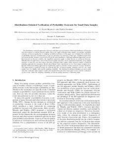
types), higher-order types (types depending on types), dependent types (types depending on terms), intersection types (terms with multiple types), etc. An elegant way to subsume some of these systems is Barendregt's How does the
λ-calculi?
λ-cube
λ-cube
[Barendregt 1992], presented in Figure 1.1.
actually work, and what is the mechanism which connects these eight
and
s, s1 , s2 ∈ S ,
Type
and
we can express the eight systems via a set of general axioms and rules (Figure
1.2) and rules speci�c to each of the systems (Figure 1.3).
(s1 , s2 )
∗ and �. In the literature Kind. If we let S = {∗, �},
First, we select two constants, called sorts, and name them
and, perhaps, more informatively, they are often known as
speci�c rule with elements of
S
Essentially, by instantiating the
and adding these instantiations to the general axioms
and rules, we can arrive to each of these eight systems. One very interesting thing which can be observed here is the apparent �modularity� of this segment of typed lambda calculi. Starting from the core rules, we can arrive to many di�erent systems and levels of expressiveness, each of them important in its own right, by adding instances
1.2. A Word on λ-calculi
11
Figure 1.1: The
λ-cube
of one single rule schema, akin to simply plugging in an add-on module, which we can also combine together. Let us examine it in more detail. The
(∗, ∗)
instantiation of
(s1 , s2 )
gives us the simply-typed
λ-calculus λ→ ,
and places us in
the bottom-left corner of the cube. From there, we can move in the following three directions: 1.
Upward:
(�, ∗) rule, we arrive at the system λ2, which is also known as the λ-calculus or Girard's System F [Girard 1972], where we can have terms with polymorphic types, such as Πα:∗.(α → α), arriving at terms depending on types, which would not be possible in λ→ . Also, since here we can derive ` Πα:∗.(α → α) : ∗, we by adding the
second-order typed
e�ectively bring impredicativity (self-referencing) back in the game whenever we introduce type polymorphism (the four systems on the top side of the cube). 2.
Forward: such as
by adding the
λα:∗.α → α
(�, �) rule,
we arrive at the system
λω ,
where type constructors
(types depending on types) can be formed and used to create new
higher-order constructors and types, which cannot be used in
λ→
or
λ2.
The systems
allowing higher-order constructions are on the back side of the cube. 3.
Sideways:
by adding the
(∗, �) rule, we arrive at the system λP , where we have dependent
types, or types depending on terms.
Here, we can, for instance, capture the notion of
predicates, and have derivations such as kind of predicates on
A),
The remaining three systems (λ2P , presented here, with
λC ,
A:∗ ` (A → ∗) : �
(meaning that
A→∗
is the
which is not possible in any of the previous systems.
λω
and
λC )
are combinations of the four which we have
which is also known as the Calculus of Constructions, being the most
expressive one and combining all of the demonstrated features. One may view typed
λ-calculi
as an interesting and amusing theoretical exercise. However,
perhaps somewhat unexpectedly, they share a fundamental connection with mathematical logic and have very important applications in computer science. Typed lambda calculi are, in fact, in the foundations of programming languages, and form the base of typed functional programming languages such as Haskell and ML, as well as, albeit more indirectly, typed imperative programming languages.
12
1.2.3
Chapter 1. Introduction
Figure 1.2: The general axioms and rules for the
λ-cube
Figure 1.3: The speci�c axioms and rules for the
λ-cube
The Curry-Howard Correspondence
It was �rst noticed, by Haskell Curry [Curry 1934], that the types of some of the combinators (K and
S,
for example) in the simply-typed
λ-calculus
could be seen as axiom schemata for in-
tuitionistic implicational logic. Some twenty years later [Curry 1958], he concluded that Hilbertstyle deduction systems correspond, in some fragment, to the typed fragment of combinatory logic, while Howard [Howard 1980] was the �rst to state that intuitionistic natural deduction can directly be interpreted as a typed variant of the
λ-calculus.
This observation is known as
the Curry-Howard correspondence. Essentially, it tells us that two formalisms which we need
1.3. Interactive Theorem Proving and the Proof Assistant Coq
13
not have expected to be similar - lambda calculi (as models of computation) and mathematical logics (as proof systems) - are structurally the same. Through the Curry-Howard correspondence, we arrive at the important notion of propositions-
as-types, meaning that propositions of a proof system correspond to types within a typed
λ-
calculus. In that case, if the proposition is provable in the proof system, the corresponding type will be inhabited in the
λ-calculus,
and the term inhabiting it can be seen as its proof. Even
further, this term can be seen as an executable program. The logics corresponding to the systems of the in a format similar to the
λ-cube
λ-cube
and the relationships between them,
(called the logic cube), are shown in Figure 1.4. All of the
logics of the logic cube are intuitionistic.
PROP
Propositional logic (PPL)
PROP2
Second-order PPL
PROPω
Weakly higher-order PPL
PROPω
Higher-order PPL
Predicate logic (PRL)
PRED2
Second-order PRL
Weakly higher-order PRL
PREDω
Higher-order PRL
PRED PREDω
Figure 1.4: The Logic Cube
1.3 Interactive Theorem Proving and the Proof Assistant Coq An interactive theorem prover or a proof assistant is a software tool that allows the user to describe within it concepts such as mathematical theories or programming languages, formulate a certain problem or state certain properties with respect to that concept, and specify a solution or verify that that property holds. The proving process is guided by the user and assisted by the proof assistant, in the sense that the user provides the steps and the proof assistant veri�es that these steps are correct.
The steps themselves mostly mimic pen-and-paper reasoning,
and involve concepts such as proof by induction or contradiction, case analysis, application of already proven theorems, and many more.
While parts of the proof within a proof assistant
can be automated, it is the user who concentrates on the creative details and truly guides the proving process, separating clearly proof assistants from automated theorem provers, whose task is to autonomously construct the entire proof. The proofs produced using automated and interactive theorem provers have a higher degree of certainty when compared to pen-and-paper proofs, because they rely on a trusted core - a
14
Chapter 1. Introduction
collection of code on which the theorem prover is based, that is small enough to be manually veri�able, that is declared correct, and upon which all of the subsequent inferences are made. This higher degree of certainty is required in �elds and contexts (such as medicine, aviation, robotics and security) where software faults could introduce a life-threatening risk. Currently, there is a number of interactive theorem provers available to researchers, all essentially de�ned by their respective underlying formalisms. The Curry-Howard correspondence has paved way for the development of several of them, while the others rely on set theory and higher-order logic. Here is a non-exhaustive list of the most widely used proof assistants today:
• ACL2 - A Computational Logic for Applicative Common Lisp
[Kaufmann 2000]
is a software system consisting of a programming language, an extensible theory in a �rstorder logic, and a mechanical (capable of working in both interactive and automatic modes) theorem prover, in the Boyer-Moore tradition [Boyer 1995].
It is designed to support
automated reasoning in inductive logical theories, mostly for the purpose of software and hardware veri�cation.
• Agda
[The Agda development team 2013] is a proof assistant for developing constructive
proofs as well as a functional programming language with dependent types. It is based on the idea of the Curry-Howard correspondence. It has a certain degree of support for tactics and proofs are dominantly written in functional programming style. The language has ordinary programming constructs such as data types, pattern matching, records, let expressions and modules, and a Haskell-like syntax.
• Coq [The
Coq development team 2013, Bertot 2004] is based on an extension of
λC known
as the Calculus of Inductive Constructions [Coquand 1988, Paulin-Mohring 1996], and is, therefore, at the very �top� of the
λ-cube
when it comes to expressiveness. It allows the
expression of mathematical assertions, is capable of mechanically checking proofs of these assertions, allows the use of various tactics for the �nding of these formal proofs, and can extract a certi�ed program from the constructive proof of its formal speci�cation. It has been developed over the past two decades in the French National Institute for Research in Computer Science and Control (INRIA). Coq is written in a typed functional language called Objective CaML, an extension of the core Caml language with a fully-�edged objectoriented layer, also developed in INRIA.
• HOL [Gordon
2013] (Higher Order Logic) denotes a family of interactive theorem proving
systems sharing similar (higher-order) logics and implementation strategies. Systems in this family are implemented as a library in some programming language.
This library
implements an abstract data type of proven theorems so that new objects of this type can only be created using the functions in the library which correspond to inference rules in higher-order logic.
As long as these functions are correctly implemented, all theo-
rems proven in the system must be valid.
The latest system from this family is HOL4
[The Hol4 development team 2013].
• Isabelle [The
Isabelle development team 2013] is an interactive theorem prover, successor
of the HOL theorem prover. It is written in Standard ML, and is based on a small logical core guaranteeing logical correctness. Isabelle is generic: it provides a meta-logic (a weak type theory), which is used to encode object logics like First-order logic (FOL), Higherorder logic (HOL) or Zermelo-Fraenkel set theory (ZFC). Isabelle's main proof method is a higher-order version of resolution, based on higher-order uni�cation. Though interactive, Isabelle also features e�cient automatic reasoning tools, such as a term rewriting engine and a tableaux prover, as well as various decision procedures.
1.3. Interactive Theorem Proving and the Proof Assistant Coq • PVS
15
[The PVS development team 2013] is a mechanized environment for formal speci�-
cation and veri�cation. PVS consists of a speci�cation language, a number of prede�ned theories, a type checker, an interactive theorem prover that supports the use of several decision procedures and a symbolic model checker, various utilities including a code generator and a random tester, documentation, formalized libraries, and examples that illustrate di�erent methods of using the system in several application areas. It is based on a kernel consisting of an extension of Church's type theory with dependent types, and is fundamentally a classical typed higher-order logic.
• Twelf
[The Twelf development team 2013] is language used to specify, implement, and
prove properties of deductive systems such as programming languages and logics. It features dependent types, relies on the Curry-Howard correspondence and is based on the calculus and the
LF
λP
logical framework.
Let us now take a more detailed look into the inner workings of Coq, the proof assistant relevant for this thesis. Coq o�ers a variety of tools and mechanisms for encoding and veri�cation:
• All the tools of λC . As the basis of Coq is the Calculus of Inductive Constructions, which subsumes λC , we have immediately at our disposal dependent types, polymorphism, and higher-order constructions. All of the objects in Coq have a type, and even types have their own types, which we call sorts.
In Coq, there are two sorts:
Type
and
Prop,
the
former applicable to data, and the latter for logical propositions.
• Inductive types.
Using inductive types, i.e. by de�ning types through a case-by-case
description of the type, with possibly making use of previously constructed terms of that type, it is possible to naturally encode notions such as natural numbers, integers, lists, binary trees, propositional formulas, and virtually any structure inductive in nature. For instance, we would encode natural numbers as
Inductive nat : Type = 0 : nat | S : nat -> nat.
• Induction.
As a mechanism for proving assertions over inductive types, structural in-
duction is one of the built-in mechanisms of Coq. Furthermore, it is possible to de�ne a custom induction principle, which, of course, has to �rst be proven correct.
• Proof tactics.
There is a number of methods for proof simpli�cation, or tactics, readily
available. Some of these tactics involve simple manipulations on the syntactic and semantic levels of higher-order intuitionistic logic and equality (intros,
apply or reflexivity), inversion) or the
whereas others involve more complicated mechanisms (induction or
use of computational tools (omega).
• Records. jects.
Coq also provides support for records, which are essentially collections of ob-
Using records, we can, for instance, elegantly exploit dependent types to express
side conditions of a certain type. We will illustrate this on the following example:
Record typeRestriction (U : Type) (W : U -> Prop) : Type := mkTypeRes {origU :> U; inW : W origU}. where, starting from a given type
typeRestriction U W
U
and its subset
W
we have constructed a new type
which contains only the elements of
three things we can notice about this de�nition: tures dependent types (since the type of
W
U
which are in
it is parametric over
depends on the term
U,
U
W. and
There are
W,
it fea-
and the type of the
16
Chapter 1. Introduction origU), and it also features another of Coq's useful mechanisms, which is coercion, denoted by :>, which tells the system that objects of type typeRestriction U W can be treated, if necessary, as objects of type U.
condition
inW
depends on the term
• In�nite objects.
In addition to inductive types, Coq also o�ers co-inductive types,
which allow reasoning about in�nite objects while still remaining in the �nite con�nes of a computer. Some of the objects we can construct in this manner are streams, lazy lists and lazy binary trees, whereas one of the notions we can capture using co-inductive types is bisimilarity.
• Modules.
Coq provides pre-formalized collections of facts, lemmas, and theorems regard-
ing various topics, such as set theory, number theory and linear algebra, all organized in importable modules. The user can also de�ne his own modules, which can be compiled and re-used across developments. As the underlying logic of Coq is intuitionistic, there exists a module (Classical) which adds the double negation elimination axiom to the axiom pool, making it possible to reason in classical terms.
• Program extraction.
Coq has the possibility to extract certi�ed and e�cient functional
programs from either Coq functions or Coq proofs of speci�cations. The output language of these programs can be Objective CaML, Haskell or Scheme. One of the most signi�cant, and one of the currently most complex examples of program extraction is the CompCert C certi�ed compiler of C-light (a large subset of the C language), intended for compilation of life-critical and mission-critical software [Leroy 2009a] [Leroy 2009b].
• CoqIDE.
Last, but not least, Coq comes with a graphical user interface called CoqIDE,
which is highly interactive, giving the user an overview of the current proof code, the state of the current proof, and the options at his disposal. So far, many important and fundamental theorems have already been proven in Coq, such as the denumerability of rational numbers, the non-denumerability of the continuum, Gödel's Incompleteness Theorem, the Cayley-Hamilton theorem.
Stirling's formula, etc.
However, as
the most important ones we could single out the Four Color Theorem (stating that, given any separation of a plane into contiguous regions, producing a map, no more than four colors are required to color the regions of the map so that no two adjacent regions have the same color) [Gonthier 2004] or, more recently, the Feit-Thompson Theorem (stating that every �nite group of odd order is solvable) [Gonthier 2012]. In conclusion, we present a very simple illustrative proof in Coq, showing that the well-known
(A → (B → C)) → ((A → B) → (A → C)) is indeed a tautology. The claim is stated Lemma, the name of which is example, and the syntax of the formulation is quite intuitive.
formula as a
Parentheses are written mostly for the bene�t of the reader, as most of them are not needed, due to the built-in associativity of the intuitionistic implication.
Prop
is the sort for propositions.
Lemma example : forall A B C : Prop, (A -> (B -> C)) -> ((A -> B) -> (A -> C)). Proof.
// The proof context is empty at this point, and our goal is stated in the format encountered after the name of the lemma.
intros A B C.
// The proposition has to hold for all A, B and C of sort Prop (boolean values - true and false). Hence, we can pull them into the context as A : Prop, B : Prop, and C : Prop, leaving us with the formula without the leading forall part as the goal.
intros Habc Hab Ha. // We usually prove an implication of the form A -> B by assuming to have A as an assumption, and then attempting to prove B, given that assumption. Here, we have several implication which we can pull back into the context as assumptions Habc : A -> (B -> C) is the first one, followed by Hab : A -> B, and Ha : A, leaving only C in the goal.
1.4. Probability, λ-calculus, and Formal Veri�cation
17
apply Habc.
// Also, if we have to prove a goal C, and we have an assumption of the form A -> C, it would be sufficient to prove A. Here, given that we have an assumption A -> (B -> C), it would be sufficient to prove A and to prove B. This splits the goal in two - one for A, one for B.
assumption.
// We already have A in the assumptions.
apply Hab.
// Similarly as before, our goal is B, and we already have A -> B in the hypotheses. Therefore, to prove our goal, it would be sufficient to prove A.
assumption.
// We already have A in the assumptions.
Qed.
// All the goals have been proven.
1.4 Probability, λ-calculus, and Formal Veri�cation Several works on the treatment of probability in
λ-calculi,
as well as formal veri�cation of
algorithms and programs involving probability and/or randomness can be found in the literature. In [Park 2006], the authors have presented a probabilistic language, called
λ◦ ,
which uni-
formly supports all types of probability distributions - discrete, continuous, and even those not belonging to either group. Its mathematical basis are sampling functions, i.e. , mappings from the unit interval
λ◦
(0, 1]
to probability domains. They have also described the implementation of
as an extension of Objective CAML and demonstrated its practicality with three applications
in robotics, with experiments carried out with real robots. In [Hurd 2002], where the proof assistant of choice was HOL, the author starts with an extensive formalization of measure theory and probability spaces. Next, using that formalization, the author proceeds to de�ne the notion of a probabilistic program that terminates with probability 1, and shows, both in theory and by example, how probabilistic programs can be speci�ed and formally veri�ed in that setting. In [Hurd 2005], the authors present a mechanization of the quantitative logic for the guarded command language pGCL [Morgan 1999], using the HOL theorem prover. pGCL is a language which allows for the expression of both probabilistic and demonic (arbitrary) choices, and it is suitable for reasoning about distributed random algorithms. The authors show that the mechanized theory supports the creation of an automatic proof tool which takes as input an annotated pGCL program and its partial-correctness speci�cation, and derives from that a su�cient set of veri�cation conditions. Finally, in [Audebaud 2009], the authors rely on [Hurd 2002] and [Park 2006] to be able to reason in a formal setting (the proof assistant Coq) about properties of randomized algorithms, namely the validity of general rules for estimating the probability that a randomized algorithm satis�es a speci�ed property. In this thesis, the formalization of the mathematics surrounding probability theory has been executed on a smaller scale than in [Hurd 2002], on a need-to-have basis (con�ned to �nitely additive measures), while probabilistic programs are not addressed, and the emphasis in put on meta-theoretic properties of probability logics.
Part I
Probability Logics
Chapter 2
LPCP - A Probability Logic with
Conditional Probability Operators Contents
2.1 2.2 2.3 2.4 2.5 2.6 2.7 2.8
Syntax and Semantics of LPCP . . . . . . An Axiomatization of LPCP . . . . . . . . Soundness of LPCP . . . . . . . . . . . . . Strong Completeness of LPCP . . . . . . . Decidability of LPCP . . . . . . . . . . . . An Interlude: Reasoning about Evidence Representing Evidence with LPCP . . . . Summary . . . . . . . . . . . . . . . . . . .
. . . . . . . .
. . . . . . . .
. . . . . . . .
. . . . . . . .
. . . . . . . .
. . . . . . . .
. . . . . . . .
. . . . . . . .
. . . . . . . .
. . . . . . . .
. . . . . . . .
. . . . . . . .
. . . . . . . .
. . . . . . . .
. . . . . . . .
. . . . . . . .
. . . . . . . .
. . . . . . . .
22 24 26 26 31 33 33 34
LPCP is a probability logic with multiple conditional probability operators, based on classical logic. Here, we present its syntax and semantics, together with a corresponding strongly complete axiomatization.
LPCP
is the outcome of a research e�ort which has followed the lines of
investigation presented in [Maksimovi¢ 2008, Ognjanovi¢ 2009, Fagin 1990, Lukasiewicz 2002, Ra²kovi¢ 2004, Ognjanovi¢ 2005] on the formal development of probability logics, in which probability-related statements can be expressed using probabilistic operators which specify bounds on probabilities of a propositional formulas. The work presented here originated from [Maksimovi¢ 2008], which has been presented at the
13th
ESSLLI Student Session in Hamburg,
in 2008, and which developed into a journal publication [Doder 2010], published in the Publications de l'Institut Mathematique, in 2010. As mentioned in the previous paragraph, in operators
LPCP
we have multiple conditional probability
CPi , i ∈ I , where I denotes a �nite non-empty set of indexes. These operators take as α and β , and produce as output the conditional probability that α
input two classical formulas holds if
β
holds. One interpretation which could be given to these operators is that each of them
represents an agent which has his own independent assessment of the conditional probability of an event. For instance, we would be able to formally write the statement �The conditional
α α given γ
β
probability of an event
given an event
probabilities of
viewed by agent
viewed by agent
j
and twice
γ
i
is at least the sum of conditional
given
α
viewed by agent
k .�
as
CPi (α, β) > CPj (α, γ) + 2 · CPk (γ, α). We provide the syntax and semantics of
LPCP,
accompanied with a strongly complete ax-
iomatization. We also prove that the developed logic is decidable, and show that it can be used to represent evidence, solving the problem of propositional axiomatization of reasoning about evidence, which has been presented in [Halpern 2006]. Before we examine the logic in detail, we will address a minor issue which is well-known in probability theory. In the classical Kolmogorovian sense, the conditional event � α given
β�
can
22
Chapter 2. A Probability Logic with Conditional Probability Operators
be considered only in the case when
P (β) > 0,
and for such a conditional event, we calculate its
probability in the following way:
P (α|β) = P (α ∧ β) · P (β)−1 .
(2.1)
−1 operator is not total, since
0 does not have an inverse, this approach could introduce di�culties into the formal construction of probabilistic formulas, and it would be better if P (α|β) were to be a well-de�ned term, regardless of the α, β , and the possible value of P (β). As the
We can reach an elegant solution to the situation by adopting the convention that
−1 is a
total operation, so that we can extend Kolmogorov's de�nition of conditional probability onto
P (α|β) = P (α ∧ β)P (β)−1 .
all of the events:
In particular, if
P (β) = 0,
then
P (α ∧ β) = 0,
and
P (α|β) = P (α ∧ β)P (β)−1 = 0 · P (β)−1 = 0. 0−1 is P (β) = 0 the
If we look closely at this last equation, we can observe that the actual value of essentially irrelevant for the computation of
P (α|β),
and that in the case when
conditional probability de�ned as above does indeed behave correctly. For the sake of simplicity, we will take
0−1
to be equal to
1.
The remainder of this chapter is organized as follows: in Section 2.1, the syntax of the logic
LPCP
is presented and the class of measurable probabilistic models is described. Section 2.2
contains the corresponding axiomatization and introduces the notion of deduction. A proof of the strong completeness theorem for
LPCP
is presented in Section 2.4, whereas the decidability
of the logic is analyzed in Section 2.5. Representing evidence in
LPCP
is discussed in Section
Section 2.7, and the concluding remarks are in Section 2.8.
2.1 Syntax and Semantics of LPCP Let
V ar = {pn | n < ω}
be the set of propositional variables.
propositional formulas over
V ar
will be denoted by
F orC ,
The corresponding set of all
and is de�ned as the smallest set
which satis�es the following conditions: 1. it contains all of the propositional variables, i.e.
V ar ⊂ F orC ,
2. it is closed under the following rules of construction: if then
¬α
and
Here, we will take
α∧β
α and β
are propositional formulas,
are propositional formulas.
¬ and ∧ to be the basic propositional connectives, and we de�ne the remaining
connectives in the usual manner for classical propositional logic. Propositional formulas will be denoted by
α, β
De�nition 1.
and
γ,
The set
possibly with indexes. Next, let
T erm
I
be a �nite non-empty set of indexes.
of all probabilistic terms is recursively de�ned as follows:
• T erm(0) = {s | s ∈ Q} ∪ {CPi (α, β) | α, β ∈ F orC , i ∈ I}. • T erm(n + 1) = {f, (f + g), (s · g), (−f) | f, g ∈ T erm(n), s ∈ Q}. • T erm =
∞ S
T erm(n).
n=0 Probabilistic terms will be denoted by
h, possibly with indexes. To simplify our f + g will represent (f + g), f + g + h will Pn represent ((f + g) + h). For n > 3, i=1 fi will represent ((· · · ((f1 + f2 ) + f3 ) + · · · ) + fn ). Similarly, −f will represent (−f) and f − g will represent (f + (−g)). The intended meaning f, g
and
notation, we introduce the following convention:
2.1. Syntax and Semantics of LPCP
23
behind probabilistic terms is for them to represent linear combinations of rationally-weighted conditional probabilities, in the sense that each term can be rewritten (using the axioms and inference rules from the next Section, which essentially correspond to the axioms of rational numbers) into an expression of the form
�X n
� si · CPi (αi , βi ) + s.
(2.2)
i=1
α CPi (α, β)
Finally, if term
and
β
are propositional formulas, and
i ∈ I,
then we will have the probabilistic
to be read as �the conditional probability of
further simplify the notation, we will be writing
Pi (α)
α
β viewed by agent i�. To CPi (α, >), where > denotes
given
instead of
an arbitrary tautology instance.
De�nition 2.
A basic probabilistic formula is any formula of the form
f > 0.
The set of all
probabilistic formulas is de�ned as the smallest set which satis�es the following conditions: 1. it contains all of the basic propositional formulas, 2. it is closed under the following rules of construction: if then
¬f
and
f∧g
f
and
g
are propositional formulas,
are propositional formulas.
As in the case of propositional formulas, illustrated above, here we also treat
¬
and
∧
as the
primitive connectives, while all of the other connectives are introduced in the usual way, as in classical propositional logic. Probabilistic formulas will be denoted by indexes, while the set of all probabilistic formulas will be denoted by
φ, ψ and θ, possibly with F orP . Furthermore, we
de�ne the following abbreviations: 1.
f60
represents
−f > 0.
2.
f>0
represents
¬(f 6 0).
3.
f 0).
4.
f=0
represents
f 6 0 ∧ f > 0.
5.
f 6= 0
represents
¬(f = 0).
6.
f>g
represents
f − g > 0.
We de�ne
f 6 g, f > g, f < g, f = g
and
f 6= g
in a similar way. By �formula�, we will be
referring to either a propositional formula or a probabilistic formula. We do not allow for the mixing of propositional and probabilistic formulas, nor for the nesting of probability operators
α ∧ CPi (β, γ) ≥ 0 or formulas such as CPi (CPj (α, β), γ) in LPCP. Formulas will be denoted by Φ, Ψ and Θ, possibly with indexes. The set of all of the formulas will be denoted by F or . Next, we proceed to the semantics of LPCP. We de�ne the notion of a model as a special kind of Kripke model. Namely, a model M is any quadruple hW, H, {µi | i ∈ I}, vi such that:
CPi .
Therefore, it is not possible to have formulas of the form
• W
is a non-empty set. As usual, we will be referring to its elements as worlds.
• H
is an algebra of sets over
•
for each
W.
i ∈ I , µi : H −→ [0, 1]
is a �nitely additive probability measure.
• v : F orC × W −→ {0, 1} is a truth assignment compatible v(¬α, w) = 1 − v(α, w) and v(α ∧ β, w) = v(α, w) · v(β, w).
with
¬
and
∧.
That is,
24
Chapter 2. A Probability Logic with Conditional Probability Operators
For a given model
M,
we will denote by
the context is clear, we will write
[α] ∈ H
for all
w ∈ W such that v(α, w) = 1. say that M is a measurable model
the set of all
instead of
[α]M .
We
If if
α ∈ F orC .
De�nition 3.
Let
|=
bility relation
[α]
[α]M
be any measurable model. We de�ne the satis�a-
recursively as follows:
1.
M |= α
2.
M |= f > 0
if
M = hW, H, {µi | i ∈ I}, vi
v(α, w) = 1 if
for all
fM > 0,
where
w ∈ W. fM
is recursively de�ned in the following way:
• sM = s. • CPi (α, β)M = µi ([α ∧ β]) · µi ([β])−1 ,
for any
i ∈ I.
• (f + g)M = fM + gM . • (s · g)M = s · gM . • (−f)M = −(fM ). 3.
M |= ¬φ
4.
M |= φ ∧ ψ
if
M 6|= φ. if
M |= φ
and
M |= ψ .
Φ is satis�able if there exists a measurable model M = hW, H, {µi | i ∈ I}, vi that M |= Φ; Φ is valid if it is satis�ed in every measurable model. We say that the set formulas is satis�able if there is a measurable model M such that M |= Φ for all Φ ∈ T .
A formula such
T
of
The reader can notice that the last two clauses of De�nition 3 guarantee the validity of each tautology instance.
2.2 An Axiomatization of LPCP In this section, we will introduce the axioms and inference rules for of our axiomatic system, which we denote by
AXLPCP ,
LPCP.
The set of axioms
is divided into three groups: axioms for
propositional reasoning, axioms for probabilistic reasoning, and arithmetical axioms.
Axioms for propositional reasoning:
A1a. τ (p1 , . . . , pn ) - all tautologies instantiated with propositional formulas A1b. τ (Φ1 , . . . , Φn ) - all tautologies instantiated with probabilistic formulas Axioms for probabilistic reasoning (i
A2. A3. A4. A5. A6. A7.
∈ I ):
Pi (α) > 0. Pi (>) = 1. Pi (⊥) = 0. Pi (α ↔ β) = 1 → Pi (α) = Pi (β). Pi (α ∨ β) = Pi (α) + Pi (β) − Pi (α ∧ β). P (β) = 0 → CP (α, β) = 0;
Capturing conditional probability:
Non-negativity of probability Something true will always occur Something false will never occur Equivalent formulas are equally probable The inclusion�exclusion principle Disallowing division by zero
2.2. An Axiomatization of LPCP
25
(Pi (α ∧ β) ≥ r ∧ Pi (β) ≤ s) → CPi (α, β) ≥ r · s−1 , −1 , A9. (Pi (α ∧ β) > r ∧ Pi (β) ≤ s) → CPi (α, β) > r · s −1 , A10. (Pi (α ∧ β) ≥ r ∧ Pi (β) < s) → CPi (α, β) > r · s −1 , A11. (Pi (α ∧ β) ≤ r ∧ Pi (β) ≥ s) → CPi (α, β) ≤ r · s −1 , A12. (Pi (α ∧ β) < r ∧ Pi (β) ≥ s) → CPi (α, β) < r · s −1 , A13. (Pi (α ∧ β) ≤ r ∧ Pi (β) > s) → CPi (α, β) < r · s A8.
s 6= 0. s 6= 0. s 6= 0. s 6= 0. s 6= 0. s 6= 0.
Arithmetical axioms: A14. A15. A16. A17. A18. A19. A20. A21. A22. A23. A24. A25. A26. A27. A28. A29. A30.
r > s, whenever r > s. r > s, whenever r > s. s · r = sr. s + r = s + r. f + g = g + f. (f + g) + h = f + (g + h). f + 0 = f. f − f = 0. (r · f) + (s · f) = r + s · f. s · (f + g) = (s · f) + (s · g). r · (s · f) = r · s · f. 1 · f = f. f > g ∨ g > f. (f > g ∧ g > h) → f > h. f > g → f + h > g + h. (f > g ∧ s > 0) → s · f > s · g. f = g → (φ(. . . , f, . . .) → φ(. . . , g, . . .)).
Compatibility of Compatibility of Compatibility of Compatibility of
> with > of Q ≥ with ≥ of Q · with · of Q, part + with + of Q
1
Commutativity of +
+
Associativity of
0
is the neutral for
+
+ · with + Distributivity of + with · Compatibility of · with · of Q, Neutrality of 1 Totality of ≥ Transitivity of ≥ Compatibility of ≥ with + Compatibility of ≥ with · Inverse terms for
Distributivity of
part 2
Contextual closure for terms
Inference rules:
α→β
R1. From
α
and
R2. From
α
infer
β;
infer
Pi (α) = 1,
from
for all
R3. From the set of premises
φ
and
φ→ψ
infer
ψ.
i ∈ I.
{φ → f > −n−1 | n = 1, 2, 3, . . . }
infer
φ → f > 0.
Let us brie�y comment on the axioms and inference rules. The axioms A2 through A6 provide the required properties of probability, the axioms A7 through A13 capture Equation 2.1, using the fact that
Q is dense in R, while the axioms A14 through A30 provide the properties required
for computation. As for the inference rules, R1 is modus ponens for classical and probabilistic formulas, R2 resembles necessitation, while the in�nitary rule R3 ensures that non-Archimedean probabilities are not permitted. Using the rule R3, we are able to syntactically deal with the
1 of
inherent non-compactness
LPCP and achieve strong completness.
Also, we can see that there
exist two levels of formulas - propositional and probabilistic, and that these levels are separate, in the sense that it is possible to cross from the propositional to the probabilistic level using the inference rule R2, but there is no mechanism to provide a crossing in the opposite direction.
De�nition 4
(Derivability)
.
A formula
Φ
is derivable from a set of formulas
there is an at most countable sequence of formulas or a formula from the set Particularly, a formula 1
In
LPCP,
Φ
T,
Φ0 , Φ1 , . . . , Φ,
or it is derived from the preceding formulas by an inference rule.
is a theorem (`
Φ)
if it is deducible from the empty set of hypotheses.
it is possible to construct a set of formulas that is not satis�able, but whose every �nite subset is {φ → f > 0} ∪ {φ → f < −n−1 | n = 1, 2, 3, . . . }.
satis�able. An example of this set is the set
2
such that every
T 2 (T ` Φ) if Φi is an axiom
We refer to formulas in
T
as assumptions or hypotheses.
26
Chapter 2. A Probability Logic with Conditional Probability Operators
De�nition 5
(Consistent and Inconsistent Sets)
at least one formula from
T.
Otherwise,
De�nition 6
T
F orC
.
A set of formulas
and at least one formula from
F orP
T
is consistent if there is
that are not deducible from
is inconsistent.
.
(Maximally Consistent Sets)
A consistent set
T
of sentences is said to be maxi-
α ∈ F orC , it holds that if T ` α then α ∈ T φ ∈ F orP , either φ ∈ T or ¬φ ∈ T .
mally consistent if for every
for all
i ∈ I,
and for every
De�nition 7 T ` Φ,
(Deductively Closed Sets)
.
A set
T
and
(Pi (α) = 1) ∈ T ,
is deductively closed if for every
Φ ∈ F or,
if
Φ ∈ T.
then
With the presented axioms and inference rules, one can notice that the length of the inference may be any successor ordinal lesser than the �rst uncountable ordinal in�nite (countable) proofs in
ω1 ,
i.e. that we can have
LPCP.
2.3 Soundness of LPCP The �rst meta-theoretical result we will prove about our logic will be the soundness theorem, which follows easily from the formulation of the axiom system and the inference rules.
Theorem 1
(Soundness)
.
If
Φ
is a theorem of
AXLPCP ,
then it is valid.
Proof. Essentially, we need to prove that the instances of all of the axioms of
AXLPCP
are valid,
and that applications of the inference rules preserve validity. As the axiom schemes are checked to be valid in the usual manner, we will focus on the application of the inference rules:
α and α → β are valid. This means that α and α → β ≡ ¬(α ∧ ¬β) are true in every world w ∈ W of every model M = hW, H, {µi |i ∈ I}, vi. However, since we have that ¬(α ∧ ¬β) is true, then it must be that β is true,
R1. Let us assume that the classical formulas
which concludes this part of the proof. The part for the modus ponens for probabilistic formulas is proven similarly.
α is valid. This means that α is true in every M = hW, H, {µi |i ∈ I}, vi. Therefore, we have that [α] = W , µi ([α]) = µi (W ) = 1, for all i ∈ I . This, in turn, means that
R2. Let us assume that the classical formula world
w∈W
of every model
meaning that we have that
M |= Pi (α) = 1,
which concludes this part of the proof.
{φ → f ≥ −n−1 | n = 1, 2, 3, . . .} is valid, i.e. that for every model M = hW, H, {µi |i ∈ I}, vi, it holds that M |= {φ → f ≥ −n−1 | n = 1, 2, 3, . . .}. Now, if M 6|= φ, then M |= φ → f ≥ 0 immediately,
R3. Let us assume that the set of probabilistic formulas
as the antecedent of the (classical) implication is false.
Therefore, let us assume that
M |= φ. Then, given the de�nition of implication via conjunction and negation, we have −1 | n = 1, 2, 3, . . .}, and we need to prove that M |= f ≥ 0. Given the that M |= {f ≥ −n M ≥ 1 | n = 1, 2, 3, . . .}, and we need to prove de�nition of satis�ability, we have that {f n M that f ≥ 0, which follows from the axiomatization of real numbers.
2.4 Strong Completeness of LPCP In this section, we will prove that the proposed axiomatization is strongly complete with respect to the class of all measurable models. As is quite common, the �rst step to take is to prove the Deduction Theorem.
2.4. Strong Completeness of LPCP Theorem 2 or
.
(Deduction theorem)
Φ, Ψ ∈ F orP .
Then, it holds that
27
T be an arbitrary set of formulas, T ` Φ → Ψ i� T ∪ {Φ} ` Ψ.
Let
and let
Φ, Ψ ∈ F orC
T ` Φ → Ψ. From this, regardless of whether Φ and Ψ are T ∪{Φ} ` Φ → Ψ. However, we also have that T ∪{Φ} ` Φ. Therefore, using the appropriate modus ponens (inference rule R1), we obtain that T ∪ {Φ} ` Ψ. Conversely, let T ∪ {Φ} ` Ψ. We proceed by structural induction on this inference with the goal of proving T ` Φ → Ψ. In case when the last applied rule was R1, the proof proceeds just as
Proof. First, let us assume that
classical or probabilistic, we have that
for classical logic. Next, let the last applied rule be the inference rule R2. In that case, we have that
Ψ is of the form Pi (α) = 1, for some i ∈ I , which was obtained from T ∪ {Φ} ` α.
However,
as the classical and probabilistic formulas are separate, the derivation of classical formulas does
T ` α. From there, using the inference T ` Pi (α) = 1. From here, using the tautology φ0 → (φ1 → φ0 ) and the axiom A1b, we obtain the desired T ` Φ → (Pi (α) = 1). Finally, let the last applied rule be R3. Then, Ψ is of the form φ → f > 0 and we have, −1 ) for all n. Since the formula by the induction hypothesis, that T ` Φ → (φ → f > −n (φ0 → (φ1 → φ2 )) ↔ ((φ0 ∧ φ1 ) → φ2 ) is a tautology, we also have that T ` (Φ ∧ φ) → f > −n−1 , for all n, with the help of the axiom A1b. Now, by the inference rule R3, we have that T ` (Φ ∧ φ) → f > 0, and by using the same tautology as above, that T ` Φ → Ψ. With this proof, the reader can appreciate why the `φ →' �pre�x� in needed in the rule R3 � without it, not depend on probabilistic formulas, and we have that rule R2, we obtain that
we could not have used the tautology required for the crucial application of the rule R3. We will use the result of the next technical lemma in the construction of a maximally consistent extension of a consistent set of formulas.
Lemma 1.
T
Let
T ∪ {φ → f > 0} is T ∪ {φ → f < −n−1 } is consistent.
be a consistent set of formulas. If
exists a positive integer
n
such that
inconsistent, then there
T ∪ {φ → f < −n−1 } is inconsistent for all positive −1 } ` ⊥. From positive integers n, T ∪ {φ → f < −n
Proof. Let us assume the converse, i.e. that integers
n.
Therefore, we have that, for all
this, using the Deduction Theorem, we have that
T ` φ → f > −n−1 , for all positive integers so we have that
T
n.
Now, using the inference rule R3, we have that
T ` φ → f > 0,
and
must be inconsistent, which is in contradiction with our original assumption,
therefore completing our proof.
De�nition 8.
T
be a consistent set of formulas, and let us have an enumeration of proba3 ∗ bilistic formulas, i.e. let F orP = {φi | i ∈ ω} . We de�ne a completion T of T as follows: 1.
Let
T0 = T ∪ {α ∈ F orC | T ` α} ∪ {Pi (α) = 1 | T ` α, i ∈ I}.
2. If
Ti ∪ {φi }
is consistent, then
3. If
Ti ∪ {φi }
is inconsistent, then:
(a) If
φi
(b) Otherwise, 4
ψ → f > 0, then Ti+1 = Ti ∪ {ψ → f < −n−1 }, 4 such that Ti+1 is consistent .
is of the form
positive integer
3
Ti+1 = Ti ∪ {φi }.
Ti+1 = Ti .
This is possible, as probabilistic formulas are countable by construction. The existence of such an
n
is provided by Lemma 1.
where
n
is a
28
Chapter 2. A Probability Logic with Conditional Probability Operators 4.
T∗ =
S∞
n=0 Tn .
Ti
We can prove that each that
T∗
Theorem 3.
Let
1. For each 2.
3.
T∗
is consistent by construction. In the next theorem, we will prove
is maximally consistent and deductively closed.
T
be a consistent set of formulas, and let
φ ∈ F orP ,
either
φ ∈ T∗
or
be constructed as above. Then:
¬φ ∈ T ∗ .
is consistent, i.e.
(a) There is a formula
α ∈ F orC ,
such that
α∈ / T ∗.
(b) There is a formula
φ ∈ F orP ,
such that
φ∈ / T ∗.
T∗
T∗
is deductively closed, i.e. if
T∗ ` Φ
then
Φ ∈ T ∗.
Proof. 1. Let us assume the opposite: let
¬φ ∈
T ∗ , or neither
φ ∈
φ
be a probabilistic formula such that both
T ∗ nor
that, in the above enumeration,
¬φ ∈ φ ≡ φi
T ∗.
Tk+1 ` φ ∧ ¬φ,
i.e. that
Tk+1
second case, by construction, we have that
and
Without loss of generality, we can assume
¬φ ≡ φj , and let k = max(i, j). Then, Tk+1 ` φ, and Tk+1 ` ¬φ. However, then
and
construction, in the �rst case, we have that also have that
φ ∈ T∗
by we
is inconsistent, which is not possible. In the
Tk+1 ∪ {φ} ` ⊥,
and that
Tk+1 ∪ {¬φ} ` ⊥.
From this, using the Deduction Theorem and the elimination of double negation, we again obtain that
Tk+1 2.
Tk+1 ` φ, and Tk+1 ` ¬φ, and from that, we have that Tk+1 ` φ ∧ ¬φ, i.e. that
is inconsistent, which is still not possible, and we have our claim.
(a) Since there are no classical formulas added during the formation of
T ∗,
all of the
∗ classical formulas which are in T are also in T0 . Therefore, if it were to hold that ∗ all classical α are in T , then all classical α would also have to be in T0 , making it inconsistent by de�nition, which is not the case. Therefore, there must be a classical formula
α,
such that
α∈ / T.
(b) This is a direct consequence of item 1. At this point, taking into consideration the manner in which e�ectively proven that
T∗
T0
is constructed, we have
is maximally consistent.
3. We will proceed by structural induction on the derivation of
T ∗ ` Φ.
Φ ∈ T0 ⊆ T ∗ . Otherwise, Φ ∈ F orP , and there is a non-negative integer i such that Φ ≡ φi of the ∗ above enumeration. Then, since ` Φ, it must be that Ti ` φi and so Φ ∈ Ti+1 ⊆ T .
(a) Let
Φ
(b) Let
T∗ ` Φ ≡ β
be an instance of an axiom. Then, if
be obtained from
T∗ ` α
Φ ∈ F orC
T∗ ` α → β α→β∈T β ∈ T0 ⊆ T ∗ .
and
∗ R1. Then, by the construction of T , we have that there, by the construction of
T0 ,
we have that
we have that
by the inference rule and
α ∈ T,
and from
T ∗ ` Φ ≡ φ be obtained from T ∗ ` ψ and T ∗ ` ψ → φ by the inference rule R1, and let ψ ≡ φi , ψ ≡ φj , and φ → ψ ≡ φk in the above enumeration. Then, φ is a deductive consequence of each Tl , where l > max(i, k) + 1. Next, let ¬φ ≡ φm . If φm ∈ Tm+1 , then ¬φ is a deductive consequence of each Tn , where n > m + 1. Therefore, for every n > max(i, k, m) + 1, we would have that Tn ` φ ∧ ¬φ, which is ∗ a contradiction with the consistency of Tn . Thus, it must be that ¬φ 6∈ T . However, ∗ given item 1, it must then be that φ ∈ T .
(c) Let
2.4. Strong Completeness of LPCP
i ∈ I be obtained from T ∗ ` α by the inference rule R2. However, this means that T ` α and, by the construction of T0 , we have ∗ that Pi (α) = 1 ∈ T0 ⊆ T for all i ∈ I .
(d) Let
T ∗ ` Φ ≡ Pi (α) = 1,
29
for some
T ∗ ` φ → f > −n−1 , for all n ≥ 0. −1 ∈ T ∗ , for all n ≥ 0. By the induction hypothesis, we then have that φ → f > −n / T ∗. Next, let φ → f > 0 = φi in the above enumeration, and let us assume that φi ∈ Then, Ti ∪ {φi } must be inconsistent, which means that, for some positive integer n, φ → f < −n−1 ∈ Ti+1 , according to item 3a of De�nition 8. Next, let φ → f ≥ −n−1 ≡ φj in the above enumeration. Then, for all k ≥ max(i, j) + 1, we have that Tk ` φ → f < −n−1 and Tk ` φ → f ≥ −n−1 , which is in contradiction with the consistency of Tk . Therefore, it must be that Φ ∈ T , and we have our claim.
(e) Let
T∗ ` Φ ≡ φ → f > 0
be obtained from
Next, for a given consistent set of formulas set
T ∗, 1.
we proceed to de�ne a canonical model
W
w : F orC −→ {0, 1}
is the set of all functions
• w
is compatible with
• w(α) = 1
for each
2.
v : F orC × W −→ {0, 1}
3.
H = {[α] | α ∈ F orC }.
4.
µi : H −→ [0, 1]
Lemma 2. M ∗
¬
α∈
T and its completion to a maximally consistent M ∗ = hW, H, {µi |i ∈ I}, vi as follows: with the following properties:
∧.
and
T ∗.
is de�ned by
is de�ned by
v(α, w) = 1
i�
w(α) = 1.
µi ([α]) = sup{s ∈ [0, 1] ∩ Q | T ∗ ` Pi (α) > s},
for all
i ∈ I.
is a measurable model.
Proof. Here, we need to prove that
H
is an algebra of sets and that each
µi
is indeed a �nitely
[α]∩[β] = [α∧β], H \ [α] = [¬α], from which we obtain that H is an algebra of sets. Concerning the measures µi , the non-negativity requirement (µi ([α]) ≥ 0) is the consequence of axiom A2 and the de�nition of µi , while the requirement that µi (W ) = 1 follows directly from the axiom A3, since W = [>]. Now, we will turn our attention to the proof of �nite additivity. Let µi ([α]) = a, µi ([β]) = b and µi ([α ∧ β]) = c. What we would like to prove is that additive probability measure. Given the properties of the measure, we have that
[α] ∪ [β] = [α ∨ β]
and
µi ([α ∨ β]) = a + b − c. Since the set of rational numbers Q is dense in R, we can choose an increasing sequence a0 < a1 < a2 < · · · and a decreasing sequence a0 > a1 > a2 > · · · in Q such that lim an = lim an = a. Using the de�nition of µi and item 1 of Theorem 3, we obtain that T ∗ ` Pi (α) > an ∗ ` P (φ) < a , for all positive integers n. In the same way, we can also choose and that T i n increasing sequences (bn )n∈ω and (cn )n∈ω , and decreasing sequences (bn )n∈ω and (cn )n∈ω in Q, such that lim bn = lim bn = b and lim cn = lim cn = c. For these sequences, we have that T ∗ ` Pi (β) > bn ∧ Pi (β) < bn and T ∗ ` Pi (α ∧ β) > cn ∧ Pi (α ∧ β) < cn . From here, using the arithmetical axioms, we have that
T ∗ ` Pi (α) + Pi (β) − Pi (α ∧ β) > an + bn − cn and
T ∗ ` Pi (α) + Pi (β) − Pi (α ∧ β) < an + bn − cn
30
Chapter 2. A Probability Logic with Conditional Probability Operators n. Using the axioms A6 and A30, we obtain that T ∗ ` Pi (α ∨ β) > T ∗ ` Pi (α ∨ β) < an + bn − cn , for all n. Finally, from the fact that
for all positive integers
an + bn − cn
and that
µi ([α ∨ β]) = sup{r ∈ Q | T ∗ ` Pi (α ∨ β) > r} and
lim an + bn − cn = lim an + bn − cn = a + b − c,
we obtain that
µi ([α ∨ β]) = a + b − c.
Now, we are ready to prove the main theorem:
Theorem 4 Proof. Let ∗
T
T
.
Every consistent set of formulas has a measurable model.
(Strong Completeness)
be a consistent set of formulas. We can extend it to a maximally consistent set
, and de�ne a canonical model
M ∗,
induction on the complexity of the formulas. First, we prove that if
M ∗ |= α. ` α, and α ∈ T ∗ .
1. As the base case, let
∗ have that T
M ∗ |= f > 0,
M ∗ |= Φ i� Φ ∈ T ∗ M ∗ |= Φ, then Φ ∈ T ∗ :
as above. We will now prove that
by
By the completeness of classical propositional logic, we
∗
f M ≥ 0. If f > 0 ∈ / T ∗ , from the construction of T ∗ , there exists −1 ∈ T ∗ . But then, by the construction of M ∗ , we a positive integer n, such that f < −n ∗ M < 0, which is a contradiction. Therefore, we have that f > 0 ∈ T ∗ . would have that f
2. Let
3. Let we
i.e.
M ∗ |= ¬φ. Then, by de�nition of |=, we get that M ∗ 6|= φ. By the induction hypothesis, ∗ ∗ have that φ 6∈ T , and �nally, by item 1 of Theorem 3, we have that ¬φ ∈ T .
4. Finally, let
M ∗ |= φ ∧ ψ .
|=, we have that M ∗ |= φ and M ∗ |= ψ . φ, ψ ∈ T ∗ , and �nally, by item 3 of Theorem 3,
Then, by de�nition of
By the induction hypothesis, we get that we have that
φ ∧ ψ ∈ T ∗.
T ∗ ` CPi (α, β) ≥ r implies that µi ([αi ∧βi ])µi ([βi ])−1 ≥ r. Indeed, if it were that µi ([αi ∧ βi ])µi ([βi ])−1 < r, there would exist a, b ∈ Q, such that a > µi ([αi ∧ βi ]), b ≤ µi ([βi ]), and µi ([αi ∧ βi ])µi ([βi ])−1 < ab < r. Using the previously proven ∗ ∗ direction, we would have that T ` Pi (α ∧ β) < a and T ` Pi (β) ≥ b, and hence, by A12, ∗ −1 that T ` CPi (α, β) < a · b , which would be a contradiction. Similarly, we can show that ∗ T ` CPi (α, β) ≤ r implies that µi ([αi ∧ βi ])µi ([βi ])−1 ≤ r. As a consequence, we have that µi ([αi ]|[βi ]) = sup{r ∈ Q | T ∗ ` CPni (α, β) > r}. Next, we proceed to prove the opposite ∗ ∗ direction: if Φ ∈ T , then M |= Φ: Here, it is important to notice that that
1. As the base case, let
M∗
Φ = α ∈ F orC .
If
α ∈ T ∗,
i.e.
T ∗ ` α,
then, by de�nition of
M ∗,
|= α.
2. Let us suppose that
f > 0 ∈ T ∗.
Then, using the axioms A16�A19, A22�A25 and A30, we
can prove that
T∗ ` f = s +
m X
si · CPni (αi , βi )
and
T∗ ` s +
i=1 for some
s, si ∈ Q
m X
si · CPni (αi , βi ) > 0,
i=1
and some
αi , βi ∈ F orC , ni ∈ I .
This is not surprising, given the
intended design of terms (cf. Equation 2.2). Moreover, given the axioms A7, A16, A20 and A30, we can e�ectively cancel out all of the subterms of
f in which we have conditional ∗ probabilities CPi (α, β) with Pi (β) = 0, and, therefore, may assume that T ` Pni (βi ) > 0. Next, let
ai = µni ([αi ∧ βi ])
and
bi = µni ([βi ]).
s+
m X i=1
We need to prove that
si · ai · b−1 i > 0.
(2.3)
2.5. Decidability of LPCP
31
dec (cinc i,k )k∈ω and decreasing sequences (ci,k )k∈ω −1 inc dec in Q, such that lim ci,k = lim ci,k = ai bi , for i ∈ {1, . . . , m}. Hence, we have that dec T ∗ ` CPni (α, β) > cinc i,k ∧ CPni (α, β) < ci,k , for i ∈ {1, . . . , m} and k ∈ ω .
Therefore, we can choose increasing sequences
Without loss of generality, we can assume that for
l < i 6 m.
Then, using the arithmetical axioms, we obtain that
T∗ ` s +
l X
and
∗
T `s+
l X
si · cdec i,k 6 s +
m X
si ·
cdec i,k
m X
+
si · CPni (αi , βi )
i=1
i=l+1
i=1
k.
m X
si · cinc i,k +
i=1
for all
T ∗ ` si > 0, for 1 6 i 6 l, and T ∗ ` si < 0,
si ·
cinc i,k
>s+
m X
si · CPni (αi , βi )
i=1
i=l+1
Consequently, we have that
m X
s+
si · ai ·
b−1 i
∗
= sup{r ∈ Q | T ` s +
m X
si · CPni (αi , βi ) > r}.
i=1
i=1
Now, Equation 2.3 follows from
T∗ ` s +
m X
si · CPni (αi , βi ) > 0.
i=1 3. Let
¬φ ∈ T ∗ .
Then, by item 1 of Theorem 3, we have that
∗ hypothesis, we have that M ∗ that M |= ¬φ. 4. Finally, let
6|= φ,
Φ = φ ∧ ψ ∈ T ∗.
φ 6∈ T ∗ .
Next, by the induction
and �nally, by the de�nition of satis�ability, we obtain
Then, by item 3 of Theorem 3, we have that
∗ Next, by the induction hypothesis, we have that M |= ∗ de�nition of satis�ability, we obtain that M |= φ ∧ ψ .
φ
∗ and M
|= ψ ,
φ, ψ ∈ T ∗ .
and �nally, by the
2.5 Decidability of LPCP Theorem 5.
Satis�ability of probabilistic formulas is decidable.
Proof. Up to equivalence, every probabilistic formula is a �nite disjunction of �nite conjunctions of literals, where a literal is either a basic probabilistic formula, or a negation of a basic probabilistic formula. Thus, it would be su�cient to show the decidability of the satis�ability problem for formulas of the form
^
^
fi > 0 ∧
i Suppose that
A1 , . . . , A2n
p1 , . . . , pn
gj < 0.
(2.4)
j
are all of the propositional letters appearing in Equation 2.4.
Let
be all of the formulas of the form
±p1 ∧ · · · ∧ ±pn , where
+p = p
and
−p = ¬p.
We can see that
>.
Furthermore, for each classical formula
set
Iα ⊆ {1, . . . , 2n }
α
Ai
are pairwise-disjoint and form a partition of
appearing in Equation 2.4, there exists a unique
such that
α↔
_ i∈Iα
Ai
32
Chapter 2. A Probability Logic with Conditional Probability Operators
is a tautology. Now, given Equation 2.2, we can equivalently rewrite Equation 2.4 as
^X i
sii0 CPni0
i0
� _
Ak ,
> ri ∧
Al
^X j
l∈Iβ
k∈Iαii0
Let the set
�
_ ii0
{i1 , . . . , im } ⊆ I
indexes which appear in Equation 2.4, and let
� s
ii0
k∈Iαii0 ∩Iβ
�
Furthermore, let
Al
< rj .
jj 0
σi (x(1,i1 ) , . . . , x(2n ,i1 ) , . . . , x(1,im ) , . . . , x(2n ,im ) ),
l∈Iβ
ii0
� � X �−1 x(k,nj 0 ) · x(l,nj 0 ) < rj .
X
sjj 0 ·
j0
l∈Iβ
be the formulas
ii0
and
X
Ak ,
k∈Iαjj 0
�
� � X �−1 x(k,ni0 ) · x(l,ni0 ) > ri
X
·
i0
j0
_
be the set of all of the di�erent conditional probability operator
δj (x(1,i1 ) , . . . , x(2n ,i1 ) , . . . , x(1,im ) , . . . , x(2n ,im ) ) X
sjj 0 CPnj 0
� _
k∈Iαjj 0 ∩Iβ
l∈Iβ
jj 0
jj 0
χ(x(1,i1 ) , . . . , x(2n ,i1 ) , . . . , x(1,im ) , . . . , x(2n ,im ) ) ^
^
x(1,ih ) + · · · x(2n ,ih ) = 1 ∧
be the formula
x(k,ih ) > 0.
k,h
h∈{1,...,m}
Then, we can notice that Equation 2.4 is satis�able if and only if the sentence
∃x(1,i1 ) . . . ∃x(2n ,i1 ) . . . ∃x(1,im ) . . . ∃x(2n ,im )
�^
σi (¯ x) ∧
i is satis�ed in the ordered �eld of reals. contain �
^
� δj (¯ x) ∧ χ(¯ x)
(2.5)
j
Formally, the �rst order language of �elds does not
−1 � and � −�. However, both of these functions are easily de�nable. For instance, � −1 �
can be de�ned by the following formula:
ϕ(x, y) : (x = 0 → y = 1) ∧ (x 6= 0 → xy = 1), (∀x)(∃1 y)ϕ(x, y) is satis�ed in every �eld. In particular, the −1 formula ψ(. . . , x , . . .) holds if and only if the formula ψ(. . . , y, . . .) ∧ ϕ(x, y) holds. Therefore,
since the �rst order sentence
Equation 2.5 can be seen as a �rst-order formula belonging to the language of ordered �elds
LOF
� de�nitions by extensions, see [Shoen�eld 1967]. Based on results presented in [Marker 2002], we have that the satis�ability of sentences of
LOF
in the ordered �eld of reals is decidable.
0−1 = 1 does not a�ect the aforementioned reasoning, as the conditional probability of α given β is equal to 0 i� the probability of α ∧ β is equal to 0, regardless of the value of the probability of β . It should be noted here that our choice to extend the operation
−1 so that
Now, let us suppose that there is only one conditional probability operator, i.e. that there exists only one agent. It should be noted that this logic can be embedded into the logic described in [Fagin 1990], which has a PSPACE containment for the decision procedure. Also, the rewriting of formulas from our logic into that logic can be accomplished in linear time:
CP (α, β)
is equivalent to
which can be represented easily in [Fagin 1990].
ω(α∧β) ω(β) ,
Furthermore, the generalization of the logic
from [Fagin 1990] to a multi-agent case is straightforward. Therefore, we conclude that our logic is also decidable in PSPACE.
2.6. An Interlude: Reasoning about Evidence
33
2.6 An Interlude: Reasoning about Evidence Imagine the following scenario: we have two coins, one of which is fair (with a head on one side and a tail on the other, with the probability of
50%
for each of the outcomes), while the other
one is extremely biased (e.g. with a probability of only
1%
for the tail to appear on top). We
also have the results of a series of tosses originating from one of the coins, but we do not know which. Furthermore, we have no information whatsoever regarding prior probability assigned to the choice of the coin, and we would like to make some sort of probabilistic inference as to which coin has actually been tossed only from the results of the tosses. Then, we can view these results as evidence in favor of or against one of the coins, and it is precisely this notion that we would like to model. The model should capture our intuition about the matter in question. For instance, if we were to have a series of 50 tosses with only three tails, we could induce that the coin in question is the biased one, while if we were to have a series of 50 tosses with 24 heads and 26 tails, we could induce that the coin in question is the fair one. The topic of evidence has been discussed comprehensively in philosophical literature, namely philosophy of science and, more precisely, con�rmation theory, where the main topic of discussion is the extent to which experimental evidence lends credence to various scienti�c theories [Good 1950, Popper 1959, Carnap 1962, Milne 1996]. There are three things which a framework capturing evidence should incorporate: probabilistic outcomes (such as the outcome of the actual coin toss), non-probabilistic outcomes (such as the choice of the coin toss), and, mainly, the change in likelihood of a hypothesis caused by the previous probabilistic outcomes. While there were many research e�orts which have successfully been able to capture the �rst two requirements [Halpern 1993, de Alfaro 1997, He 1995], it was not until [Halpern 2006] that the third one was also realized.
2.7 Representing Evidence with LPCP In [Halpern 2006], Halpern and Pucella have presented a �rst-order logic for reasoning about evidence. It includes propositional formulas on hypotheses and
P2
vation
H,
observations
of formulas before and after the observation, the evidence
o
for the hypothesis
h,
O,
probabilities
P1
E(o, h) provided by the obser-
and quanti�cation by real-valued variables. They have posed an
open question whether it would be possible to axiomatize their logic without using quanti�cation. Intuitively, the evidence function
e represents the �weight�
with which an observation leads
to the ful�llment of a hypothesis. Also, it was shown that evidence can be seen as a function which maps prior probability
P1
to posterior probability
P2 ,
using Dempster's Rule of Combi-
nation. For more details, we refer the reader to [Halpern 2006]. In this section, we will show how evidence can be represented using
LPCP.
We will introduce the following modi�cations:
V ar = H ∪ O, O = {o1 , . . . , on } are used to
1. There is a �nite number of propositional letters divided into two categories: where
H = {h1 , . . . , hm }
denote observations, and
are used to denote hypotheses,
H ∩ O = ∅.
2. There are only two conditional probability operators �
CP1
and
CP2 ,
which will be inter-
preted as prior and posterior conditional probabilities, respectively; 3. there is an additional syntactic object � 4. The de�nition of
T erm(0)
E(o, h),
where
o ∈ O , h ∈ H.
is adjusted accordingly to:
T erm(0) = {s | s ∈ Q} ∪ {CPi (α, β) | α, β ∈ F orC , i ∈ I} ∪ {E(o, h)|o ∈ O, h ∈ H}.
34
Chapter 2. A Probability Logic with Conditional Probability Operators 5. The de�nition of a model is extended to be a sextuple have
e : ({[o]|o ∈ O} × [{[h]|h ∈ H}]) → [0, 1]
hW, H, {µi |i ∈ I}, v, ei,
where we
by the formula
µ1 ([o ∧ h]) · µ1 ([h])−1 , −1 k=1 µ1 ([o ∧ hk ]) · µ1 ([hk ])
e([o], [h]) = Pm for
o ∈ O, h ∈ H.
6. The de�nition of satis�ability is extended to include:
M
E(o, h)
M
= (CP1 (o, h) ) ·
�X m
CP1 (o, hk )
M
�−1 ,
k=1 for
o ∈ O, h ∈ H.
7. There are nine additional axioms:
A33.
Wm V ( i=1 hi ) ∧ ( i6=j (hi → ¬hj )). Wn V ( i=1 oi ) ∧ ( i6=j (oi → ¬oj )). Vn i=1 (CP1 (oi , h1 ) + . . . + CP1 (oi , hm ) > 0).
A34.
(CP1 (oi , hj ) > r ∧ CP1 (oi , h1 ) + . . . + CP1 (oi , hm ) 6 s) → E(oi , hj ) > r · s−1 .
A35.
(CP1 (oi , hj ) > r ∧ CP1 (oi , h1 ) + . . . + CP1 (oi , hm ) < s) → E(oi , hj ) > r · s−1 .
A36.
(CP1 (oi , hj ) > r ∧ CP1 (oi , h1 ) + . . . + CP1 (oi , hm ) 6 s) → E(oi , hj ) > r · s−1 .
A37.
(CP1 (oi , hj ) 6 r ∧ CP1 (oi , h1 ) + . . . + CP1 (oi , hm ) > s) → E(oi , hj ) 6 r · s−1 .
A38.
(CP1 (oi , hj ) 6 r ∧ CP1 (oi , h1 ) + . . . + CP1 (oi , hm ) > s) → E(oi , hj ) < r · s−1 .
A39.
(CP1 (oi , hj ) < r ∧ CP1 (oi , h1 ) + . . . + CP1 (oi , hm ) > s) → E(oi , hj ) < r · s−1 ,
A31. A32.
8. There is one additional inference rule:
R4.
oi , i ∈ {1, . . . , n}, j ∈ {1, . . . , m}. P2 (hj ) = CP1 (hj |oi )
It can be shown, very similarly to the already laid-out proofs, that the logic with these modi�cations in place is also strongly complete and decidable in PSPACE. In this way, we have solved the problem of propositional axiomatization of reasoning about evidence, which was presented in [Halpern 2006].
2.8 Summary In this chapter, we have introduced a sound and strongly-complete axiomatic system for a probability logic with conditional probability operators
CPi , i ∈ I ,
LPCP-
which allows for linear
combinations and comparative statements. As it was noticed in [van der Hoek 1997], it is not possible to provide a �nitary strongly complete axiomatization for such a system. In our case, the strong completeness was made possible by adding an in�nitary rule of inference. The formalism which we have obtained is fairly expressive and allows for the representation of uncertain knowledge, where uncertainty is modeled by probability formulas. We have shown it to be decidable, and also that it can be extended in order to be used to represent evidence, making it the �rst propositional axiomatization of reasoning about evidence.
Chapter 3
Formal Veri�cation of Key Properties for LP P2Q - a Rationally-valued Probability Logic without Iterations in the Proof Assistant Coq Contents
3.1 3.2 3.3 3.4
Syntax of LP P2Q . . . . . . . Semantics of LP P2Q . . . . . . A Complete Axiomatization Key Properties of AxLP P . Q 2
. . . .
. . . .
. . . .
. . . .
. . . .
. . . .
. . . .
. . . .
. . . .
. . . .
. . . .
. . . .
. . . .
. . . .
. . . .
. . . .
. . . .
. . . .
. . . .
. . . .
. . . .
. . . .
. . . .
. . . .
. . . .
. . . .
35 37 39 41
3.4.1
Soundness . . . . . . . . . . . . . . . . . . . . . . . . . . . . . . . . . . . . .
41
3.4.2
Completeness . . . . . . . . . . . . . . . . . . . . . . . . . . . . . . . . . . .
42
3.4.3
Non-Compactness
49
3.4.4
Concerning Decidability
. . . . . . . . . . . . . . . . . . . . . . . . . . . . . . . . . . . . . . . . . . . . . . . . . . . . . . . . . . . . .
49
3.5 Summary . . . . . . . . . . . . . . . . . . . . . . . . . . . . . . . . . . . . . 50 LP P2Q - a probability logic that extends classical logic with probabilistic operators of the form P≥ rα, with the meaning that the probability that the classical formula α holds is at least r . This logic does not allow iterations of probability operators. We In this chapter, we introduce
present its syntax and semantics, as well as a strongly complete axiomatic system. We formally prove its main meta-theoretical properties (soundness, strong and simple completeness, and non-compactness) using the proof assistant Coq.
3.1 Syntax of LP P2Q In the logic
LP P2Q , there exist two types of formulas:
classical and probabilistic. For the classical
φ = {p0 , p1 , . . .}, and The set of all classical formulas F orC is then de�ned
formulas, we require a denumerably in�nite set of propositional letters: two propositional connectives:
¬c
and
→c .
as the smallest set that satis�es the following conditions:
•
it contains all of the propositional letters, and
•
is closed under the following formation rules: if
α, β ∈ F orC ,
then
¬c α, α →c β ∈ F orC .
These are, in fact, formulas as they are commonly de�ned in classical propositional logic and, as we will see in more detail later on, classical propositional logic will serve us as a base logic underneath the probabilistic level. In the encoding of classical formulas (represented by the inductive type
forC),
the propositional letters are represented by Coq's built-in type for natural
36
Chapter 3. Formal Veri�cation of the Probability Logic LP P2Q in Coq
nat, while the connectives ¬c and →c are, respectively, represented by the constructors NegC : forC -> forC and ImpC : forC -> forC -> forC. Next, let us denote by Q[0,1] the set of all rational numbers belonging to the unit interval. numbers
For the probabilistic formulas, we require a denumerably in�nite set of probabilistic operators
P≥s , s ∈ Q[0,1] , formulas
F orP
¬p
and two propositional connectives:
an expression of the form
P≥s α,
where
s ∈ Q[0,1] ,
→p . A basic probabilistic formula is α ∈ F orC . The set of all probabilistic
and
and
is then de�ned as the smallest set satisfying the following conditions:
•
it contains all of the basic probabilistic formulas, and
•
is closed under the following formation rules: if
A, B ∈ F orP ,
then
¬p A, A →p B ∈ F orP . P≥s α,
Here, the intended meaning of the probabilistic operators, using the example of
s ∈ Q[0,1] ,
and a classical formula
α,
is that the probability that
α
holds is at least
s.
for
With this,
we have constructed a new layer of formulas on top of classical logic, and within this layer we are able to assign probabilities to the classical formulas themselves. As we inspect the formation rules, we can notice that it is neither possible to combine classical and probabilistic formulas via a binary connective, nor is it possible to iterate the probabilistic operators. Therefore, in this logic, we cannot obtain formulas such as
p0 → P≥ 1 p1 2
or
P≥ 1 (P≥ 1 p0 ). 2
3
To be able to encode probabilistic formulas in Coq, we �rst require a type which could play the role of a rational number from the unit interval. This has been accomplished using
Record types,
Qc, the obtained record type Q01, and coerces to Qc. The probabilistic formulas are then represented by the inductive forP, the connectives ¬p and →p are, respectively, represented by its constructors NegP and
by imposing appropriate side conditions on the already present type is called type
ImpP
(handled analogously to their classical counterparts), and, in particular, the constructor
for probabilistic operators
P≥s
is of the form:
| Pge : Finally, the set of all formulas
Q01 -> forC -> forP
F orLP P Q 2
(represented by the inductive type
FOR)
is de�ned
as the union of all classical and probabilistic formulas:
F orLP P Q = F orC ∪ F orP . 2
Inductive FOR : Type := | Clas : forC -> FOR | Prob : forP -> FOR. Hereinafter, when we are not addressing an encoding of a concept in Coq in detail, we will specify the label of the encoding in brackets, immediately following the theoretical explanation. The remaining classical and probabilistic propositional connectives (EquC), and
∨p (OrP), ∧p (AndP), ↔p (EquP)
∨c (OrC), ∧c (AndC), ↔c
are de�ned in the usual way, while, additionally, for
the probabilistic operators, we introduce the following abbreviations: (Plt)
Ps α for ¬p P≤s α. (Pne) P6=s α for ¬p P=s α. (FalP) ⊥p for ¬p (A →p A).
(Pgt)
where we have that
(Ple)
P≤s α for P≥1−s ¬c α. P=s α for P≥s α ∧p P≤s α. (FalC) ⊥c for ¬c (α →c α).
(Peq)
s ∈ Q[0,1] , α ∈ F orC , and A ∈ F orP . α and A, respectively.
are parameterized by
We should note that
FalC
and
FalP
3.2. Semantics of LP P2Q
37
3.2 Semantics of LP P2Q The semantics for the logic
LP P2Q
is based on the possible�world approach, akin to many modal
and modal-like logics, bearing in mind that for us it is imperative to correctly capture the notion of probability expressed in the syntax.
De�nition 9.
An
LP P2Q -model
is a structure
M = hW, H, M, vi,
• W
is a non-empty set of objects we will refer to as worlds.
• H
is an algebra of subsets on
where
W.
• µ
is a �nitely additive probability measure
• v
is a valuation function
µ : H → Q[0,1] .
v : W × φ → {true, f alse},
assigning truth-values to each propo-
sitional letter in each of the worlds. It is extended to all classical formulas as usual. In this de�nition, we illustrate to what precisely the term �rationally-valued� in the title of the chapter and the description of the logic refers to, as the range of the measure, i.e. the set of values from which we are aiming to assign probabilities to classical formulas, is the set of all rational numbers belonging to the unit interval. We will provide a little more detailed look into the encoding of the semantics and the repre-
Ensemble library, which U as functions from U to Prop, Coq's sort for propositions. First, a single world
sentation of models in Coq. For representing sets, we have used Coq's treats sets of type
w∈W
is represented by:
Record ElemW (U : Type) (W : Ensemble U) : Type := mkElemW {origU :> U; inW : In _ W origU}. In this manner, and with use of Coq's dependent types, we are able to capture the property of being a member of a subset within the type, which simpli�es dealing with worlds. Now, with
Algebra function
MeasureQc being shorthand, respectively, for a set of sets of a given type U, and a U → Qc, and AOS and FAM_Qc being predicates which check, respectively, that a given
and
set of sets is indeed an algebra of subsets (i.e. that it is not empty and that it is closed under complement and union), and that a given function is indeed a probability measure on a given algebra of subsets (i.e. that it is non-negative, that the empty set measures 0, that the entire set measures 1, and that the measure itself is �nitely additive), a model is represented by:
Record Model_Simp (U : Type) (W : Ensemble U) : Type := mkMSimp {MC_Worlds : Ensemble (ElemW U W); MC_Algebra : Algebra U (ElemW U W); MC_Measure : MeasureQc U (ElemW U W); MC_Valuation : (ElemW U W) -> nat -> Prop; MC_ElemWS_Cd : inhabited (ElemW U W); MC_Worlds_Cd : MC_Worlds = Full_set (ElemW U W); MC_Is_Model : (AOS U MC_Algebra) ∧ (FAM_Qc U MC_Measure MC_Algebra)}. Therefore, apart from the four basic constituents, we have also embedded into the model the conditions which ensure that our set of worlds is not empty, that the set of worlds encompasses all of the elements of the appropriate
ElemW type, and that the algebra of subsets and the measure
meet their respective requirements. In this way, we ensure that we cannot construct a model which does not meet the required criteria. Moreover, the worlds are parameterized by a type
U,
allowing for di�erent choices of sets representing worlds, depending on the proof scenario. Here, we make use of the Coq predicate
inhabited
38
Chapter 3. Formal Veri�cation of the Probability Logic LP P2Q in Coq Inductive inhabited (A : Type) : Prop := inhabits : A -> inhabited A
that, if
A
is thought of as a type, states that there exists an element of type
use of the de�nition
Full_set
from the
Ensembles
A.
Also, note the
library
Inductive Full_set (U : Type) : Ensemble U := Full_intro : ∀x:U, Full_set U x. U.
that describes the set containing all elements of type
Empty_set
de�nition, also from the
Ensembles
Later on, we will also be using the
library
Inductive Empty_set (U : Type) : Ensemble U := . that describes the empty set of elements of type
U.
Let us proceed, after this brief detour into
LP P2Q -model M (worlds) in which α is true
formalization, with the theoretical development of the semantics. For a given
α, we will denote the set of all of the worlds {w|v(w, α) = true} by [α]M . If the model in question is clear from the subscript and write only [α] instead.
and a given formula �
De�nition 10.
An
LP P2Q -model M
[α]M ∈ H ,
is measurable if
the context, we will omit
for all
α ∈ F orC .
We will onward focus on the class of all measurable models (Model_Meas), which we will denote by
Q LP P2,M eas .
Measurable models are encoded in Coq by adding the measurability
condition into the de�nition of
De�nition 11.
Model_Simp.
The satis�ability relation
Q |=⊆ LP P2,M eas × F orLP P Q
Q conditions, for every LP P2 -measurable model
•
if
Φ ∈ F orC , M |= Φ
i�
v(w, Φ) = true,
2
M = hW, H, M, vi for all
if
Φ ∈ F orP ,
and is of the form
P≥s α, M |= Φ
and every formula
i�
all of the worlds. µ([α]M ) ≥ s.
This is how we semantically capture the notion of probability:
P≥s α
is satis�ed i� the set of worlds in which
α
a probabilistic formula
holds has the measure at least equal to
•
if
Φ ∈ F orP ,
and is of the form
¬p A, M |= Φ
•
if
Φ ∈ F orP ,
and is of the form
A →p B , M |= Φ
i�
i�
satis�ability of one probabilistic formula with the function function
modelsSet.
models,
s.
M 2 A. M 2A
or
M |= B .
In Coq, we represent the satis�ability of one classical formula with the function one formula with the function
Φ:
w ∈ W.
Classical formulas are satis�ed i� they are true in
•
satis�es the following
modelsP,
modelsC,
the
the overall satis�ability of
and the overall satis�ability of a set of formulas with the
It should be noted that the satis�ability of the negation and implication
has been encoded using Coq's built-in connectives, which operate in an intuitionistic setting. However, as we make use of theorems from Coq's
Classical library throughout the proofs, we de
facto have that they behave in a classical manner. Also, since we have delegated the evaluation of negation and implication to Coq, and didn't encode it explicitly, we can say that the encoding of
LP P2Q
presented here is a shallow encoding.
De�nition 12.
Φ is satis�able if there exists an LP P2Q -measurable model M such Q that M |= Φ; Φ is valid (Valid) if M |= Φ, for all LP P2 -measurable models M ; a set of formulas T is satis�able (Satisfiable) if there exists an LP P2Q -measurable model M such that M |= Φ, for all Φ ∈ T . A formula
3.3. A Complete Axiomatization
39
3.3 A Complete Axiomatization The set of valid formulas can be characterized by the axiom schemata presented in Figure 3.1, while the appropriate inference rules are presented in Figure 3.2. system by
AxLP P Q , 2
We denote this axiomatic
and for each axiom schema we provide a brief description of its semantics.
The main task is, once again, to have a set of axiom schemata which would allow us to easily syntactically deal with the properties of probability and the measure function.
ACT.
All instances of classical propositional tautologies for classical formulas.
APT.
All instances of classical propositional tautologies for probabilistic formulas.
AP1. P≥0 α. The probability of a formula being true is non-negative.
AP2. P≤r α →p P r. Compatibility of the probability with
≤ and forC), and an enumeration of probabilistic formulas A0 , A1 , A2 , . . . (f_enum_p : nat -> forP). Again, as in the case of the countability of the Q[0,1] interval, we take the existence of these functions as axioms in Coq. We de�ne a sequence of sets Tn (Tn_const), for n ≥ 1, as follows: � Tn ∪ {An } ∪ {P=p(αn ) αn } if Tn ∪ {An } is consistent, Tn+1 = Tn ∪ {¬p An } ∪ {P=p(¬c αn ) ¬c αn } otherwise. Next, we will be needing to establish an enumeration of classical formulas
(f_enum_c
The proof of the following lemma is based of the previously proven lemmas:
Lemma 12.
The following properties concerning the sequence
1. For all
n ≥ 0, Tn ⊆ Tn+1 (Tn_increasing).
2. For all
n ≥ 0, Tn
Tn
hold:
is consistent (Tn_all_consistent).
3. For all classical formulas
α,
if
α ∈ Tn
then
α ∈ T0 (Tn_clas_origin).
Next, we de�ne the maximally consistent extension
T∗ =
∞ [
T∗
of
T,
as
Ti .
i=1
Definition MC_Extension (T : Ensemble FOR) : Ensemble FOR := (fun A : FOR ⇒ ∃ k : nat, In FOR (Tn_const T k) A.) As can be seen, this extension is naturally de�ned in Coq as a function in only for the formulas that are contained in at least one of the extensions of captured elegantly by the existential quanti�er. For
T∗
Prop, which is true T , which has been
de�ned in this way, we prove that the
following statements hold:
Lemma 13 1. For all
T ∗ ).
(Properties of
A ∈ F orP ,
either
2.
⊥p ∈ / T ∗ (MCE_nFalP).
3.
T ⊆ T ∗ (T_in_MCE).
4. If
T ∗ ` α,
then
T0 ` α,
5. If
T ∗ ` A,
then
A ∈ T ∗,
A ∈ T∗
for
or
¬p A ∈ T ∗ (MCE_max).
α ∈ F orc (MCE_clas).
for
A ∈ F orp (MCE_prob).
Proof. 1. Directly, by construction of 2. By contradiction. If that
⊥p ∈ Tk ,
3. Directly, as
T ∗.
⊥p ∈ T ∗ ,
then, by de�nition of
T ∗,
T ⊆ T0 ,
and
T0 ⊆ T ∗ .
k, Tk .
there exists an integer
which is a contradiction with the previously proven consistency of
such
46
Chapter 3. Formal Veri�cation of the Probability Logic LP P2Q in Coq T ∗ ` α. that α ∈ Tk .
4. By induction on the structure of the derivation of
∗ de�nition of T , there exists an integer
First, if
α ∈ T ∗,
then, by
k , such Then, from Lemma 12, we T0 ` α follows immediately. Next, if α is an instance ∗ of a tautology, it automatically follows that T0 ` α. Finally, let us assume that T ` α ∗ ∗ has been obtained from T ` β and T ` β →c α, using the modus ponens for classical formulas inference rule. By the induction hypothesis, we then have that T0 ` β and that T0 ` β →c α, from which we directly obtain T ∗ → α using the modus ponens for classical obtain that
α ∈ T0 ,
from which
formulas inference rule. 5. By induction on the structure of the derivation of
T ∗ ` A.
The cases where
instance of a tautology are proven directly, as well as the cases when any of the other axioms. Next, let us assume that
∗ and T
` B → p A,
T∗ ` A
A
A
is an
is an instance of
has been obtained from
T∗ ` B
using the modus ponens for probabilistic formulas inference rule. By
B ∈ T ∗ and that B →p A ∈ T ∗ . Let i, j , and k be the values assigned to B , B →p A, and A, respectively, in the enumeration of ∗ probabilistic formulas we have used to construct T , and let m = max(i + 1, j + 1, k + 1). Then, it must hold that B , B →p A, and either A or ¬p A are are in the set Tm . However, if ¬p A ∈ Tm , then Tm would be inconsistent, as both A and ¬p A would be derivable from ∗ it. Therefore, it must be that A ∈ Tm , and, consequently, that A ∈ T . The case when A
the induction hypothesis, we then have that
has been obtained using the probabilistic necessitation inference rule is handled perhaps surprisingly easily, as then, by construction, it holds that
A ∈ T0 .
T∗ ` A →p ⊥p , and A0 ∈ F orP .
Finally, let
A0
A≡ ` →p P6=r α, for all r ∈ Q[0,1] , and some α ∈ F orC , ∗ By construction, we have that P=p(α) α ∈ T , for some integer p(α). However, by the 0 ∗ induction hypothesis, we have that A →p P6=r α ∈ T , for all r ∈ Q[0,1] , including r = p(α). 0 ∗ 0 ∗ Therefore, it must be that A ∈ / T and ¬p A ∈ T , because we would be able to �nd an inconsistent set in the sequence Tn otherwise. Now, let i and j be the values assigned to ¬p A0 and A0 →p ⊥p in the enumeration of probabilistic formulas we have used to construct T ∗ , and let m = max(i + 1, j + 1). Then, it must hold that ¬p A0 and either A0 →p ⊥p 0 or ¬p (A →p ⊥p ) are in the set Tm . However, given the tautology ¬p A →p (A →p B , if ¬p (A0 →p ⊥p ) ∈ Tm , then Tm would be inconsistent, and we have our claim. be obtained by using the domain enforcement inference rule. Then,
∗ we have that T
A0
As a direct consequence of the previous Lemma, we obtain the main result of this subsection:
Theorem 8. T ∗
is a maximally consistent set of formulas.
3.4.2.3 The Canonical Model. Now, we can turn to the construction of a canonical model formulas
T.
Worlds.
M∗
for a given consistent set of
We proceed to de�ne each of the required model components:
w be a valuation function mapping the set of propositional letters φ to {true, f alse} (nat -> Prop), and let us denote its standard extension to all classical formulas by wext . The set of worlds W (Worlds) will be the set of all valuation functions, such that their standard extensions satisfy every classical formula which is a consequence of T : Let
W = {w | w : φ → {true, f alse}, {wext (α) = 1 | α ∈ F orC , T ` α}}.
Algebra of Subsets.
We will de�ne
H (H)
in the following way:
H = {[α] | α ∈ F orC },
3.4. Key Properties of AxLP P Q
47
2
[α], as earlier, denotes the set of worlds from W in which a classical formula α is satis�ed. It is easily proven that H , de�ned in this way, satis�es the requirements to be an algebra of subsets over W : it contains the empty set (H_empty_set_in_H), it is closed under complement (H_complement_in_H), and is closed under �nite union (H_union_in_H).
where
Measure.
The measure should map the algebra of subsets
Q[0,1] . Since the elements of H are essentially µ as follows, using notation from Lemma 9: µ([α]) = q(α), Lemma 9 states that a unique
q(α)
H
into the rational unit interval
determined by classical formulas, we will de�ne
where
T ∗ ` P=q(α) α.
exists for each
α ∈ F orC ,
ensuring that the measure is
well-de�ned. The following claims needed to be proven with regard to the properties of
µ,
and
have mostly consisted of untangling a number of technical details related to properties of sets and of rational numbers:
[β] ⊆ [α],
T ` α →c β (M_included_derivable)1 .
•
If
•
Measure and negation:
•
Non-negativity:
•
Measure and the empty set:
•
Measure and the full set:
•
Additivity:
Valuation.
then
µ
µ([α]) = 1 − µ([¬c α]) (M_negation).
µ([α]) ≥ 0,
for all
α ∈ F orC (M_FAM_nonneg).
µ(∅) = 0 (M_FAM_empty_set).
µ(W ) = 1 (M_FAM_Full_set).
is �nitely additive. (M_FAM_additive).
The valuation function
v : W × φ → {true, f alse} (v)
is de�ned naturally as
v(w, pi ) = w(pi ). In this way, we have obtained a model
M ∗ = hW, H, µ, vi (Const_Model_Simp),
and the
remaining claim that we need to prove is that it is measurable.
Lemma 14. M ∗
is a measurable model (Construction_is_Measurable_Model).
Proof. We should prove that for given the construction of
α ∈ F orC ,
it holds that
[α]M ∗ ∈ H ,
which follows immediately,
H.
3.4.2.4 Strong Completeness. With the canonical model in place, we need to prove several more auxiliary lemmas on the
T
road to strong completeness. Let
be a consistent set of formulas,
T∗
denote the maximally
∗ consistent extension of T , and M denote the canonical model constructed from
Lemma 15. α ∈ T ∗ Proof. Let
M ∗ |= α.
if and only if
M ∗ |= α,
We will prove that
for all
α ∈ T0 , i.e.
T ∗.
α ∈ F orC (Cpt_iff_c).
(by de�nition of
T0 ) that T ` α, which would
be su�cient for our claim. However, we obtain this immediately from the strong completeness of classical logic.
α ∈ T ∗ . By construction of T ∗ , we have that T ` α. On the other hand, we need to prove that for all w ∈ W , v(w, α) = true. However, directly by construction ∗ of M , we have that v(w, α) = wext (α) = true, because the worlds of the canonical model are speci�cally chosen so that all of the consequences of T are true in all of the worlds. For the other direction, let
1
In the proof of this statement,
we use strong completeness of classical logic as an axiom in Coq
(LPP2_Q_Classical_Strong_Completeness_models_T).
48
Chapter 3. Formal Veri�cation of the Probability Logic LP P2Q in Coq
Lemma 16. A ∈ T ∗
if and only if
M ∗ |= A,
for all
A ∈ F orP (Cpt_iff_p).
P≥r α ∈ T ∗ . From Lemma 9 and item 2 of Lemma 8, we obtain that there exists a unique q(α) ∈ Q[0,1] , such that P=q(α) α ∈ T ∗ , while, by Theorem 8, we obtain that q(α) ≤ r. Now, given the de�nition of µ in the canonical ∗ model and the de�nition of satis�ability, we directly obtain that M |= P≥r α. For the other ∗ direction, let M |= P≥r α. Then, by construction of the canonical model and the de�nition of satis�ability, we have that r is greater than or equal to the aforementioned q(α), obtained from ∗ ∗ Lemma 9. From here, since T is maximally consistent, it has to be that T ` P≥r α. Next, let A = ¬p B . Using the induction hypothesis, our goal amounts to B ∈ / T ∗ ↔ ¬p B ∈ ∗ T , which is easily obtained from item 1 of Lemma 13. 0 0 0 / Finally, let A = A →p B . Using the induction hypothesis, our goal amounts to A ∈ ∗ 0 ∗ 0 0 ∗ 0 ∗ 0 ∗ T ∨ B ∈ T ↔ (A →p B ) ∈ T . If A ∈ / T or B ∈ T , then, by using the tautologies ¬p A →p (A → B) and B →p (A →p B), respectively, we obtain that T ` A0 →p B 0 , and, by 0 0 ∗ item 5 of Lemma 13, we obtain that A →p B ∈ T . The other direction is proven easily using A.
Proof. By structural induction on
First, let
A = P≥r α,
and let
item 1 of Lemma 13. From the previous two lemmas, we have
Lemma 17. Φ ∈ T ∗
if and only if
M ∗ |= Φ,
for all
Φ ∈ F or (Cpt_iff).
We also need the following claim:
Lemma 18.
Let
T
let us assume that
M = hW, H, µ, vi be that for all Φ ∈ F or ,
be a set of formulas and
M |= T .
Then, it holds
a measurable model, and if
T ` Φ,
then
M |= Φ
(Strong_Completeness_Consistent_T_rl).
Proof. By structural induction on the derivation of in which
Φ
T ` Φ.
The cases in which
Φ ∈ T
and
is an instance of an axiom or obtained by the modus ponens inference rules follow
directly from the soundness of the system (Theorem 6) and the induction hypothesis (IH). Next,
T ` Φ be obtained by the probabilistic necessitation inference rule. Then, we have that Φ ≡ P≥1 α, for some α ∈ F orC , and that T ` Φ was obtained from T ` α. By the IH, we have that M |= α, which means that α is true in every world, i.e. that [α] = W , i.e. that µ([α]) = 1. This, by de�nition of satis�ability, means that M |= P≥1 α, and we have our claim. Finally, let T ` Φ be obtained by the domain enforcement inference rule. Then, we have that Φ ≡ A →p ⊥p , and that T ` Φ was obtained from T ` A →p P6=r α, for all r ∈ Q[0,1] , and some α ∈ F orC , A ∈ F orP . By the IH, we have that M |= A →p P6=r α, for all r ∈ Q[0,1] . However, M |= A is not possible, since then we would have M |= ⊥p as well, which cannot be, by de�nition of satis�ability and the measure. Therefore, it must be that M 2 A, i.e. that M ` ¬p A, from which, using classical propositional tautologies, we obtain the desired M |= A →p ⊥p . let
Finally, we can prove the main result of this chapter:
Theorem 9
LP P2Q ). A set of formulas T (LPP2_Q_Strong_Completeness).
(Strong Completeness of
Q only if it is LP P2,M eas -satis�able
is
LP P2Q -consistent
if and
Theorem LPP2_Q_Strong_Completeness : ∀ T : Ensemble FOR, Consistent T Satisfiable T.
M ∗ |= T , i.e. that M ∗ |= Φ, for every formula Φ ∈ T . By Lemma 17, this is true if and only if Φ ∈ T ∗ . However, this is immediate, as every ∗ formula Φ which is in T is also, by construction, in T0 , which, in turn, is a subset of T . Next, let T be satis�able. Then, there exists a model M = hW, H, µ, vi such that M |= Φ, for all Φ ∈ T . Then, by Lemma 18, we obtain that M models all formulas derivable from T . If T were to be inconsistent, then we would have that M |= ⊥c or M |= ⊥p , which is not possible by de�nition of satis�ability, and T must be consistent.
Proof. First, let
T
be consistent. We show that
3.4. Key Properties of AxLP P Q
49
2
3.4.2.5 Simple Completeness of LP P2Q . The Simple Completeness Theorem follows naturally from the Strong Completeness Theorem, with help from the following lemma:
Lemma 19. is also
If a set of classical formulas T is LP P2Q -consistent (Cpt_ConsClas_Cons).
consistent in the sense of classical logic, then it
Proof. Directly, given strong completeness of both classical logic and
LP P2Q .
Now, we can proceed to the Simple Completeness Theorem:
Theorem 10
(Simple Completeness of
LP P2Q .).
If a formula
Φ
is
Q LP P2,M eas -valid,
then it is
Q a theorem of LP P2 . (LPP2_Q_Simple_Completeness)
Theorem LPP2_Q_Simple_Completeness : ∀ Φ : FOR, Valid Φ -> isTheorem Φ.
Φ ≡ α be a classical formula.
Proof. We have two cases to consider. First, let
Q α is LP P2,M eas {¬c α} is inconsis-
If
¬c α is not satis�able, and by the Strong Completeness Theorem, {¬c α} ` ⊥c or {¬c α} ` ⊥p . If {¬c α} ` ⊥c , then we obtain ` α from the Deduction Theorem and the elimination of double negation. If {¬c α} ` ⊥p , and {¬c α} 0 ⊥c , then we have Q that {¬c α} is classically consistent and also, by the previous Lemma, also LP P2 -consistent, valid, then
tent, i.e.
which is a contradiction.
Q A is LP P2,M eas -valid, then ¬p A is not satis�able and by the Strong Completeness Theorem, {¬p A} is inconsistent, i.e. {¬p A} ` ⊥c or {¬p A} ` ⊥p . If {¬p A} ` ⊥p , then we again obtain ` A from the Deduction Theorem and the elimination of double negation. On the other hand, if {¬p A} ` ⊥c , then since classical derivations do not depend on probabilistic formulas, it would be that ∅ ` ⊥c , which is a contradiction with the consistency of ∅, guaranteed by the Strong Completeness Theorem. Second, let
3.4.3
Φ ≡ A be a probabilistic formula.
As in the previous case, if
Non-Compactness
T = {P6=0 α}∪{P< 1 α| n ∈ N+ }. Using the domain enforcement inference n rule, we obtain that T is inconsistent (Cpc_Incons_T). By the strong completeness theorem, T is not satis�able. However, every �nite subset of T is consistent (Cpc_Finite_Sat_T), and, therefore, Q satis�able. This gives us the non-compactness theorem for LP P2 : Let us consider the set
Theorem 11
(Non-compactness of
LP P2Q ).
There exists a set of
LP P2Q -formulas
which is
unsatis�able, but whose every �nite subset is satis�able.
Theorem LPP2_Q_NonCompactness : ∃ T : Ensemble FOR, (∀ T' : Ensemble FOR, Finite _ T' → Included _ T' T → Satisfiable T') ∧ ¬ Satisfiable T. 3.4.4
Concerning Decidability
By using a method similar to that shown for
LPCP in Chapter 2, we can prove that the satis�a-
Q bility of probabilistic formulas for LP P2 is decidable, and that it is NP-complete. However, due to the perceived complexity of encoding the actual decision procedure as well as the required mathematical background in Coq, it was decided to keep the formal proof of decidability and, possibly, extraction of a certi�ed probabilistic SAT-solver, as a future research goal.
50
Chapter 3. Formal Veri�cation of the Probability Logic LP P2Q in Coq
3.5 Summary In this chapter, we have presented
LP P2Q - a rationally-valued probability logic without iterations
of probability operators. We have introduced a sound and strongly-complete axiomatic system
LP P2Q , and formally proven in Coq the main meta-theoretic properties of LP P2Q � soundness, strong and simple completeness, and non-compactness. Similarly to LPCP, due to the inherent
for
non-compactness of the system, an in�nitary inference rule had to be introduced into the system.
Chapter 4
Formal Veri�cation of Key Properties for LP P1Q - a Rationally-valued Probability Logic with Iterations - in the Proof Assistant Coq Contents
4.1 4.2 4.3 4.4
Syntax of LP P1Q . . . . . . . Semantics of LP P1Q . . . . . . A Complete Axiomatization Key Properties of AxLP P . Q 1
. . . .
. . . .
. . . .
. . . .
. . . .
. . . .
. . . .
. . . .
. . . .
. . . .
. . . .
. . . .
. . . .
. . . .
. . . .
. . . .
. . . .
. . . .
. . . .
. . . .
. . . .
. . . .
. . . .
. . . .
. . . .
. . . .
51 52 54 55
4.4.1
Soundness . . . . . . . . . . . . . . . . . . . . . . . . . . . . . . . . . . . . .
55
4.4.2
Completeness . . . . . . . . . . . . . . . . . . . . . . . . . . . . . . . . . . .
56
4.4.3
Non-Compactness
60
. . . . . . . . . . . . . . . . . . . . . . . . . . . . . . . .
4.5 Summary . . . . . . . . . . . . . . . . . . . . . . . . . . . . . . . . . . . . . 61 In this chapter, we address the logic
LP P1Q
- a probability logic similar to
LP P2Q ,
with the
main di�erence being that iterations of probability operators are allowed. We formally prove its main meta-theoretical properties in the proof assistant Coq, and discuss the di�erences in syntax, semantics and proof technology between
LP P2Q
and
LP P1Q .
4.1 Syntax of LP P1Q The syntax of
LP P1Q
is somewhat more uniform than that of
LP P2Q ,
shown in the previous
φ = {p0 , p1 , . . .} → (Imp : FOR -> FOR -> FOR), where FOR denotes the type of LP P1Q formulas in Coq. Let us again denote by Q[0,1] (Q01) Q the set of all rational numbers from the unit interval, encoded in Coq just as for LP P2 , and let us have a denumerably in�nite set of probabilistic operators P≥s , s ∈ Q[0,1] (Pge : Q01 -> FOR -> FOR). Then, the set of all formulas F orLP P Q (FOR) of LP P1Q is de�ned as the smallest set
chapter.
We also require a denumerably in�nite set of propositional letters:
(nat), and two propositional connectives:
¬ (Neg : FOR -> FOR)1
and
1
that satis�es the following conditions:
1
•
it contains all of the propositional letters.
•
if
α ∈ F or, s ∈ Q[0,1] ,
•
if
α,
then
then
P≥s α ∈ F or.
¬α ∈ F or.
Just as in the previous chapter, when we are not addressing an encoding of a concept in Coq in detail, we
will be specifying the label of the encoding in brackets, immediately following the theoretical explanation.
52
Chapter 4. Formal Veri�cation of the Probability Logic LP P1Q in Coq •
α, β ∈ F or,
if
then
α → β ∈ F or. LP P1Q
Immediately we can see the main syntactic di�erence between
LP P2Q
LP P2Q : while in LP P1Q all formulas
and
we have a separation of formulas into classical and probabilistic, in
are treated equally. The intended meaning of the probabilistic operators, using the example of
P≥s α,
for
s.
at least
s ∈ Q[0,1] ,
and a formula
α,
is still that the probability that a formula
α
holds is
As we inspect the formation rules, we can notice that it is now possible to iterate
P≥ 1 (P≥ 1 p0 ), 2 3 least 1/3, is at
the probabilistic operators. Therefore, in this logic, we can use formulas such as
p0 is at ∨ (Or), ∧ (And), and ↔ (EquC) are de�ned in the usual way,
expressing the statement that �The probability that the probability of least
1/2�.
The remaining connectives
while, additionally, for the probabilistic operators, we make use of the following abbreviations: (Plt)
Ps α (Pne) P6=s α (Pgt)
where we have that
s ∈ Q[0,1] ,
¬P≥s α. ¬P≤s α. ¬P=s α.
for for for
and
(Ple)
P≤s α for P≥1−s ¬α. P=s α for P≥s α ∧ P≤s α. (Fal) ⊥ for ¬(α → α). (Peq)
α ∈ F or.
4.2 Semantics of LP P1Q LP P1Q is based on the possible�world approach, and is somewhat Q that of LP P2 , as a result of the simpli�cation of the syntax and the
The semantics for the logic more complicated than
removal of the distinction between classical and probabilistic formulas.
De�nition 15. • W
An
LP P1Q -model
is a structure
M = hW, P rob, vi,
is a non-empty set of objects we will refer to as worlds,
• P rob is a probability assignment which assigns to each w ∈ W hW (w), H(w), µ(w)i, such that:
� W (w)
is a non-empty subset of
� H(w)
is an algebra of subsets on
� µ(w) • v
where
P rob(w) =
W. W (w).
is a �nitely additive probability measure
is a valuation function
a probability space
µ : H(w) → Q[0,1] .
v : W × φ → {true, f alse},
assigning truth-values to each propo-
sitional letter in each of the worlds. It is extended to all classical formulas as usual. As we can see, this time each of the worlds is equipped with its own subset of worlds, algebra of subsets, and measure, in contrast to
LP P2Q ,
where there was only one �general� measure
on a single algebra of subsets. This change in approach is necessary because of the possibility of iterations of probability operators. Again, the range of the measures, i.e. the set of values from which we are assigning probabilities to formulas is the set of all rational numbers from the unit interval. We will provide a detailed look into the encoding of the semantics and the representation of models in Coq, with emphasis on the di�erences from the previous chapter. First of all, the worlds and the concepts of algebras of subsets and measures are encoded in the same manner as in
LP P2Q ,
using record types (ElemW
being a member of a subset of are encoded as follows:
W,
a set of elements of
U W) capturing the property of an element type U, within the type. Probability spaces
4.2. Semantics of LP P1Q
53
Record ProbSpace (U : Type) (W : Ensemble U) : Type := mkPSpace {gWp : Ensemble (ElemW U W); gHp : Algebra (ElemW _ gWp); gMp : MeasureQc (ElemW _ gWp); PS_Nes_Cond : gWp Empty_set _; PS_Alg_Cond : AOS _ gHp; PS_Mea_Cond : FAM_Qc _ gMp gHp}. In this manner, we capture all of the necessary conditions � the non-emptiness of
H(w) H(w)
being an algebra of subsets over
W (w),
and
µ(w)
W (w),
being a �nitely additive measure on
� during the construction of a probability space. Models are then naturally encoded as:
Record Model_Simp (U : Type) (W : Ensemble U) : Type := mkMSimp {MC_Worlds : Ensemble (ElemW U W); MC_PSpace : (ElemW U W) -> (ProbSpace U W); MC_Valuation : (ElemW U W) -> nat -> Prop MC_ElemWS_Cd : inhabited (ElemW U W); MC_Worlds_Cd : MC_Worlds = Full_set (ElemW U W)}. Therefore, apart from the three required elements, we have also embedded into the model the conditions which ensure that our set of worlds is not empty and that the set of worlds encompasses all of the elements of the appropriate by a type
U,
ElemW
type. Again, the worlds are parameterized
allowing for di�erent choices of sets representing worlds, depending on the proof
scenario. Next, we proceed to the de�nition of satis�ability:
De�nition 16. model
•
M = hW, P rob, vi, if
Φ ∈ φ,
|= satis�es the following conditions, for w ∈ W , and every formula Φ ∈ F orLP P Q :
The satis�ability relation every world
M, w |= Φ
then
i�
every
LP P1Q -
1
v(w)(Φ) = true.
Propositional letters are satis�ed in a world i� they are true in that world.
•
if
Φ
is of the form
¬α, M, w |= Φ
•
if
Φ
is of the form
α → β , M, w |= Φ
•
if
Φ
is of the form
where which
i�
M, w 2 α. i�
M, w 2 α
or
M, w |= β .
P≥s α, M, w |= Φ i� µ(w)([α]M,w ) ≥ s, denotes the set {u ∈ W (w)|M, w |= α}, i.e.
[α]M,w α holds.
the set of worlds in
This is analogous to the capturing of probability for
W (w)
in
LP P2Q .
We will onward focus on the class of all measurable models (Model_Meas), which we will denote by
Q LP P1,M eas .
De�nition 17.
An
Measurable models are de�ned as follows:
LP P1Q -model M
is measurable if
[Φ]M,w ∈ H(w),
for all
Φ ∈ F orLP P Q . 1
and are encoded in Coq by adding the measurability condition into the de�nition of We represent satis�ability of a set of formulas with the function
modelsSet.
Model_Simp.
Again, we encode
satis�ability of the classical negation and implication using Coq's built-in connectives, and make use of Coq's
Classical
De�nition 18.
library.
Φ is satis�able if there exists an LP P1Q -measurable model M = hW, P rob, vi and a world w ∈ W such that M, w |= Φ; Φ is valid (Valid) if M, w |= Φ, for Q all LP P1 -measurable models M = hW, P rob, vi and all worlds w ∈ W in these models; a Q set of formulas T is satis�able (Satisfiable) if there exists an LP P1 -measurable model M = hW, P rob, vi and a world w ∈ W , such that M, w |= Φ, for all Φ ∈ T . A formula
54
Chapter 4. Formal Veri�cation of the Probability Logic LP P1Q in Coq
4.3 A Complete Axiomatization Interestingly, the set of valid formulas of
LP P1Q
can be characterized both with the same axiom
schemata presented in Figure 3.1, and the inference rules as presented in Figure 3.2, with several purely syntactic modi�cations and only one fundamental di�erence. We denote this axiomatic system by
APT.
AxLP P Q , 1
and present it in Figure 4.1 and Figure 4.2.
All instances of classical propositional tautologies.
AP1. P≥0 α. AP2. P≤r α → P r. AP3. P FOR), and de�ne a sequence
Hereinafter, we will assume to have a consistent set of formulas establish an enumeration of formulas
consistent,
The following properties concerning the sequence
1. For all
n ≥ 0, Tn ⊆ Tn+1 (Tn_increasing).
2. For all
n ≥ 0, Tn
Tn
hold:
is consistent (Tn_all_consistent).
Next, we de�ne the maximally consistent extension
T∗ =
∞ [
T∗
of
T,
as
Ti .
i=1
Definition MC_Extension (T : Ensemble FOR) : Ensemble FOR := (fun A : FOR ⇒ ∃ k : nat, In FOR (Tn T k) A.)
58
Chapter 4. Formal Veri�cation of the Probability Logic LP P1Q in Coq Again, this extension is naturally de�ned in Coq as a function in
Prop,
which is true only
∗ for the formulas contained in at least one of the extensions of T . For T de�ned in this way, we prove that the following statements hold:
Lemma 27
(Properties of
α ∈ F orLP P Q ,
1. For all
1
2.
⊥∈ / T ∗ (MCE_no_Fal).
3.
T ⊆ T ∗ (T_in_MCE).
4. If
T ∗ ).
T ∗ ` α,
then
either
α ∈ T ∗,
for
α ∈ T∗
or
¬α ∈ T ∗ (MCE_maximal).
α ∈ F orLP P Q (MCE_in). 1
Proof. 1. Directly, by construction of 2. By contradiction. If
⊥ ∈ Tk ,
T ∗.
⊥ ∈ T ∗,
then, by de�nition of
T ∗,
there exists an integer
which is a contradiction with the previously proven consistency of
3. Directly, as
T = T0 ,
and
k,
such that
Tk .
T0 ⊆ T ∗ .
4. By induction on the derivation of
T ` α.
We will only show the case where
A
has been
obtained using the probabilistic necessitation inference rule. Then, we have that the form
P≥1 β ,
and that
β
is a theorem. Next, let
enumeration of formulas. Then, since
Tn+1 = Tn ∪ β ,
β
k
be the index of the formula
β
α
is of
in the
is a theorem, and given Lemma 22, we have that
and we have our claim.
As a direct consequence of the previous Lemma, we obtain the main result of this subsection:
Theorem 14. T ∗
is a maximally consistent set of formulas.
4.4.2.3 The Canonical Model. Before we can proceed to the actual construction, we need several auxiliary lemmas:
Lemma 28. unique
Let T be a maximally consistent set. Then, for q(α) ∈ Q[0,1] , such that T ` P=q(α) α. (unique_for_M)
every
α ∈ F orLP P Q , 1
there exists a
Proof. Analogous to the proof of Lemma 9.
Lemma 29.
A formula
α
is in all maximally consistent sets if and only if
α
is a theorem.
(in_all_MCons_thm)
Proof. The right-to-left direction follows directly from the de�nition of maximal consistency. For the left-to-right direction, let us assume that for all maximally consistent sets that
α ∈ T.
First, we will prove that
that it is consistent, and let that both
¬α ∈
T 0∗
T 0 = {¬α}
T,
it holds
is inconsistent. Let us assume, to the contrary,
be its maximally consistent extension. Then, we would have
T 0∗ (by construction) and
α ∈ T 0∗
(by assumption), which is not possible, as
0∗ would not be consistent. Now, we have that then T Using the Deduction Theorem, we obtain that propositional tautologies, we obtain that
∅ ` α.
{¬α} is inconsistent, i.e. that {¬α} ` ⊥. ∅ ` ¬α → ⊥ and from there, using classical
4.4. Key Properties of AxLP P Q
59
1
Now, we can construct a canonical model
M∗
for a given consistent set of formulas
T.
Now,
we de�ne each of the required model components as follows:
Worlds.
The set of worlds
Valuation.
W
will be the set of all maximally consistent sets (CM_Worlds).
v : W × φ → {true, f alse} (v) f alse (CM_Valuation).
The valuation function
v(w, pi ) = true
if
pi ∈ w ,
Probability Space.
is de�ned naturally as
and otherwise
We will de�ne the probability spaces for each world
• Subsets of Worlds.
For each
w ∈ W,
we take
w
W (w) = W (CMWp).
as follows: This proves to be
su�cient, and there is no need for having di�erent subsets for di�erent worlds.
• Algebra of Subsets.
We will de�ne
H(w) (CMHp)
in the following way:
H(w) = {[α] = {w ∈ W : α ∈ w} | α ∈ F orLP P Q }. 1
H(w), de�ned in this way, satis�es the requirements to be an W (w): it contains the empty set, it is closed under complement, �nite union. (CM_Alg_Cond)
It is easily proven that algebra of subsets over and is closed under
• Measure. The measure should map the algebra of subsets H(w) into the rational unit interval Q[0,1] . Since the elements of H(w) are essentially determined by formulas, we will de�ne µ(w) (CMMp_to_Q01) as follows, using notation from Lemma 28: µ(w)([α]) = q(α), Lemma 28 states that a unique
q(α)
where
T ∗ ` P=q(α) α.
exists for each
α ∈ F or
, ensuring that the
LP P1Q Q measure is well-de�ned. Just as in the case of LP P2 , the following claims needed to be
proven with regard to the properties of
� � � � �
µ(w):
µ(w)([α]) = 1 − µ(w)([¬α]) (CMMp_negation). µ(w)([α]) ≥ 0, for all α ∈ F orLP P Q (CMMp_FAM_nonneg).
Measure and negation: Non-negativity:
1
µ(∅) = 0 (CMMp_FAM_empty_set). Measure and the full set: µ(W ) = 1 (CMMp_FAM_Full_set). Additivity: µ is �nitely additive (CMMp_FAM_additive). Measure and the empty set:
In this way, we have obtained a model
M ∗ = hW, P rob, vi (CMModel_Simp), and the remaining
claim that we need to prove is that it is measurable.
Lemma 30. M ∗
is a measurable model (CM_isMeas).
α ∈ F orLP P Q , and all w ∈ W , it holds that [α]M ∗ ,w ∈ H(w). 1 was how H(w) was constructed in the �rst place.
Proof. We should prove that for However, this is true, as this
4.4.2.4 Strong Completeness. With the canonical model constructed, we require an additional lemma before we can tackle strong completeness:
Lemma 31.
Let
T
be a set of formulas,
and let us assume that
M, w |= α.
M, w |= T .
M = hW, P rob, vi
w ∈ W, T ` α, then
be a measurable model,
Then, it holds that for all
α ∈ F orLP P Q , 1
if
60
Chapter 4. Formal Veri�cation of the Probability Logic LP P1Q in Coq
Proof. By structural induction on the derivation of which
T ` α.
The cases in which
α∈T
and in
α is an instance of an axiom or obtained by the modus ponens inference rule follow directly
from the soundness of the system (Theorem 12) and the induction hypothesis (IH). Next, let
T `α
α = P≥1 β , β ∈ F orLP P Q , and that β is a theorem. However, by the Soundness theorem, β is 1 then valid, i.e. M, w |= β for all w ∈ W . Therefore, we have that [β]M,w = W (w), from which we obtain that µ(w)([β]M,w ) = 1, and, consequently, that M, w |= P≥1 β , which is our claim. Finally, let T ` α be obtained by the domain enforcement inference rule. This means that α = β → ⊥, and that this was obtained from T ` β → P6=r γ , for all r ∈ Q[0,1] , and some β, γ ∈ F orLP P Q . By the IH, we have that M |= β → P6=r γ , for all r ∈ Q[0,1] . However, M |= β is 1 not possible, as by de�nition of satis�ability and the measure, it would have to be that M |= ⊥. Therefore, it must be that M 2 β , from which we easily obtain the desired M |= β → ⊥. be obtained by the probabilistic necessitation inference rule. This means that
for some
Finally, we can prove the main result of this chapter:
Theorem 15
LP P1Q ). A set of formulas T (LPP1_Q_Strong_Completeness).
(Strong Completeness of
Q only if it is LP P1,M eas -satis�able
is
LP P1Q -consistent
if and
Theorem LPP2_Q_Strong_Completeness : ∀ T : Ensemble FOR, Consistent T Satisfiable T. Proof. First, let T be consistent. We need to prove that it is satis�able, i.e. that there exists an Q LP P1,M eas -model M = hW, P rob, vi and a world w ∈ W , such that M, w |= α, for all formulas ∗
α ∈ T.
We will choose the model to be the canonical model M , while the corresponding world T ∗ , which is possible as the worlds in M ∗ are maximally consistent sets. We prove easily, ∗ ∗ ∗ by structural induction on α, that M , T |= α if and only if α ∈ T . From there, we obtain ∗ that M, w |= α, for all α ∈ T , as T ⊆ T . Next, let T be satis�able. Then, there exists a model M = hW, P rob, vi and a world w ∈ W such that M, w |= α, for all α ∈ T . Then, by Lemma 31, we obtain that M and w model all formulas derivable from T . If T were to be inconsistent, then we would have that M, w |= ⊥ which is not possible by de�nition of satis�ability, and T must be consistent. will be
4.4.2.5 Simple Completeness of LP P1Q . The Simple Completeness Theorem follows naturally from the Strong Completeness Theorem:
Theorem 16
(Simple Completeness of
LP P1Q .).
If a formula
Φ
is
Q LP P1,M eas -valid,
then it is
Q a theorem of LP P1 . (LPP1_Q_Simple_Completeness)
Theorem LPP1_Q_Simple_Completeness : ∀ Φ : FOR, Valid Φ -> isTheorem Φ. Q α is LP P1,M eas -valid, Theorem, {¬α} is inconsistent,
Proof. If
¬α is not {¬α} ` ⊥.
then
satis�able and by the Strong Completeness
i.e.
From there, we easily obtain
` α
from the
Deduction Theorem and the elimination of double negation.
4.4.3
Non-Compactness
T = {P6=0 α}∪{P< 1 α| n ∈ N+ }. Using the domain enforcement inference n rule, we obtain that T is inconsistent (Cpc_Incons_T). By the strong completeness theorem, T is not satis�able. However, every �nite subset of T is consistent (Cpc_Finite_Sat_T), and, therefore, Q satis�able. This gives us the non-compactness theorem for LP P1 : Let us consider the set
4.5. Summary Theorem 17
61
(Non-compactness of
LP P1Q ).
There exists a set of
LP P1Q -formulas
which is
unsatis�able, but whose every �nite subset is satis�able.
Theorem LPP1_Q_NonCompactness : ∃ T : Ensemble FOR, (∀ T' : Ensemble FOR, Finite _ T' → Included _ T' T → Satisfiable T') ∧ ¬ Satisfiable T.
4.5 Summary In this chapter, we have presented
LP P1Q
- a rationally-valued probability logic with iterations of
probability operators. We have introduced a sound and strongly-complete axiomatic system for
LP P1Q ,
LP P1Q � soundness, LPCP and LP P2Q , due to
and formally proven in Coq the main meta-theoretic properties of
strong and simple completeness, and non-compactness. Similarly to
the inherent non-compactness of the system, an in�nitary inference rule had to be introduced
LP P1Q and LP P2Q Q and observed that due to the more uniform syntax, the proofs in LP P1 are more elegant Q and somewhat more straightforward. Finally, the formalization of LP P1 in Coq revealed an into the system. We have examined the similarities and di�erences between
imprecision in the pen-and-paper de�nitions of the inference rules, and brought to light the need for the inference rules to be de�ned jointly with the notion of derivability.
Part II
A Logical Framework with External Predicates
Chapter 5
Introducing LFP Contents
5.1 A Brief Detour into Philosophy . . . . . . . . . . . . . . . . . . . . . . . . 66 5.2 Comparison with Related Work . . . . . . . . . . . . . . . . . . . . . . . . 68 5.3 Synopsis of the Upcoming Chapters. . . . . . . . . . . . . . . . . . . . . . 69 The Edinburgh Logical Framework
LF,
presented in [Harper 1993], is a typing system fea-
turing dependent types. It was �rst introduced as a general meta-language for logics, as well as a speci�cation language for generic proof-checking/proof-development environments. In this thesis, we consider an extension of
LF with predicates, which is accomplished by de�ning �-modality constructors, for constructing types of the
locked
type constructors, which resemble shape [ρ] , where P is predicate on typed judgements and the validity of which may be veri�ed LP N,σ outside of the LFP framework, making it, in that sense, an external predicate. Following the standard speci�cation paradigm in Constructive Type Theory, we de�ne locked types using introduction, elimination, and equality rules. We introduce a lock constructor for building objects
LP N,σ [M ]
LP N,σ [ρ], via the introduction rule (O·Lock), presented below, P destructor, UN,σ [M ], and an elimination rule (O·Unlock) which
of type
and a corresponding unlock
allows for the elimination of the locked type constructor, under the condition that a speci�c predicate
P
is veri�ed, possibly externally, on an appropriate correct, i.e. derivable, judgement.
Γ `Σ M : ρ Γ `Σ N : σ P Γ `Σ LN,σ [M ] : LP N,σ [ρ] Γ `Σ M : LP N,σ [ρ]
Γ `Σ N : σ
(O·Lock)
P(Γ `Σ N : σ)
(O·Unlock)
P [M ] : ρ Γ `Σ UN,σ The equality rule for locked types amounts to a new form of reduction we refer to as lock-
P [LP [M ]] → M , which allows for the elimination of a lock, in the UN,σ L N,σ presence of an unlock. The L-reduction combines with standard β -reduction into βL-reduction. LFP is parametric over a potentially unlimited1 set of predicates P , which are de�ned on derivable typing judgements of the form Γ `Σ N : σ . The syntax of LFP predicates is not reduction (L-reduction),
speci�ed, with the main idea being that their truth is to be veri�ed via a call to an external
validation tool ; one can view this externalization as an oracle call. Thus,
LFP
allows for the
invocation of external �modules� which, in principle, can be executed elsewhere, and whose successful veri�cation can be acknowledged in the system via
L-reduction.
Pragmatically, locked
types allow for the factoring out of the complexity of derivations by delegating the
{checking,
veri�cation, computation} of such predicates to an external proof engine or tool.
The proof
terms themselves do not contain explicit evidence for external predicates, but just record that
1
The predicates need to satisfy certain requirements so that Subject Reduction of
LFP
holds,
cf. De�nition 21.
66
Chapter 5. Introducing LFP
a veri�cation
{has
to be (lock), has been successfully (unlock)} carried out.
In this manner,
we combine the reliability of formal proof systems based on constructive type theory with the e�ciency of other computer tools, in the style of the Poincaré Principle [Barendregt 2002]. In this thesis, we develop the meta-theory of
LFP .
Strong normalization and con�uence are
proven without any additional assumptions on predicates.
For subject reduction, we require
the predicates to be well-behaved, i.e. closed under weakening, permutation, substitution, and
βL-reduction
in the arguments.
LFP
is decidable, if the external predicates are decidable. We
LFP , in the style of [Watkins 2002, Harper 2007], based of βη -long normal form. This allows for simple proofs of
also provide a canonical presentation of on a suitable extension of the notion adequacy of the encodings. In particular, we encode in
LFP
the call-by-value
λ-calculus
sion which supports the design-by-contract paradigm.
and discuss a possible exten-
We provide smooth encodings of side
conditions in the rules of Modal Logics, both in Hilbert and Natural Deduction styles, cf. [Avron 1998, Crary 2010]. We also encode sub-structural logics, namely non-commutative Linear Logic, cf. [Polakow 1999, Crary 2010]. We also illustrate how
LFP
can naturally support
program correctness systems and Hoare-like logics. We also discuss how other systems can be embedded into
LFP
via locked types and provide pseudo-code for some of the used predicates.
As far as expressiveness is concerned,
LFP
is a stepping stone towards a general theory of
shallow vs deep encodings, with our encodings being shallow by de�nition. Clearly, by Church's thesis, all external decidable predicates in codings, in standard
LF.
LFP
can be encoded, possibly with very deep en-
It would be interesting to state in a precise categorical setting the
relationship between such deep internal encodings and the encodings in
LFP
LFP .
can also be viewed as a neat methodology for separating the logical-deductive contents
from, on one hand, the veri�cation of structural and syntactical properties, which are often needlessly cumbersome but ultimately computable, or, on the other hand, from more general means of validation.
5.1 A Brief Detour into Philosophy Since Euclid �rst introduced the concept of rigorous proof and the axiomatic/deductive method, philosophers have been discussing the nature of mathematics, debating over whether it is essentially analytic or synthetic ? Although we do not presume to give comments on such a fundamental philosophical issue, we do believe that the topics in this part of the thesis could be cast against that background, and we will, therefore, o�er some comments in that direction. Several possible, albeit partial modern readings of the synthetic vs. analytic opposition could be, in our view, those of deduction from axioms vs. computation according to rules, proof checking vs. veri�cation, and proving inhabitability of judgements vs. de�nitional equality of types. The mechanism of locking and unlocking types in the presence of external oracles, which we are introducing in
LFP ,
e�ectively opens up the Logical Framework to alternate means of
providing evidence for judgements. In standard
LF,
there are only two ways of providing this
evidence, namely discovering types to be inhabited or postulating that types are inhabited by introducing appropriate constants. The locked/unlocked types of
LFP
open the door to an
intermediate level, one provided by external means, such as computation engines or automated theorem proving tools. However, among these, one could also think of graphical tools based on neural networks, or even intuitive visual arguments, as were used in ancient times for giving the �rst demonstrations of the Pythagoras' theorem, for instance. In a sense,
LFP ,
by allowing
formal accommodation of any alternative proof method to pure axiomatic deduction, vindicates all of the �proof cultures� which have been used pragmatically in the history of mathematics, and not only in the Western tradition.
5.1. A Brief Detour into Philosophy One natural objection that can be raised against the
67 LFP
framework is: �Alternative proof
methods are not rigorous enough! We need to go through the pains of rigorous formalized proof checking in order to achieve the highest possible reliability of our certi�cations!�.
While this
point is, of course, true, several points do need to be made. First of all, absolute certainty is a myth, as it cannot be achieved. The De Bruijn Principle [Barendregt 2002, de Bruijn 1968] is usually invoked in this respect. It amounts to the request that the core of the proof checker be small and veri�able by hand. Alternate proof techniques certainly do not satisfy it in a strict sense. But alternate proof techniques, if properly recorded, are not useless and come at a somewhat intermediate level between rigorous encoding and blatant axioms.
They can expedite veri�cations, as in the case of the Poincaré's Principle
[Barendregt 2002], or Deduction Modulo [Dowek 2003], or make the proof more perspicuous and provide some intuition, as Schopenhauer advocated [Shopenhauer 2008]. On a lighter note, just recall the anecdote of a famous mathematician lecturing at a seminar, who, halfway through the proof, said: �And this trivially holds!� Just to say a few seconds later: �But is it really trivial here?
Hmm. . .�.
And after about ten minutes of silence triumphantly exclaimed: �Yes, it is
indeed trivial!�. How do we encode such evidence? Should we just rule it out? Anecdote aside, there is a far deeper reason, however, why a fundamentalist approach to certainty cannot be maintained that easily, and this has to do with the issue of adequacy. Contrast, for a moment, the process of proving a computation correct with respect to carrying out its veri�cation by directly executing it. Consider, for example, that
11 ∗ 22 ∗ 33 = 108.
In the
latter case, one would need to do some simple arithmetic, while in the former case, one would need to reify the rules for computing exponentials and products. Of course, using the autarkic approach explained in [Barendregt 2002] or reasoning by re�ection as in [Chlipala 2013], one could internalize the needed arithmetics checking procedures (proving their correctness once and for all), while still preserving the de Bruijn principle and keeping proof terms small. However, our approach is more �schematic�, in the sense that it creates room for �plugging-in� any veri�er, without the need to specify which one and without the need to prove its soundness internally. But what can truly guarantee that the formalization we have encoded is adequate, i.e. that it corresponds to our intended understanding of arithmetic? Enter the Münchhausen Trilemma in all its glory. The choices we have are:
•
In�nite regression, proofs requiring more proofs, which appears because of the necessity to go ever further back. However, this isn't practically feasible and by its very nature does not provide any foundation. Just ask Achilles how his dialogue with the Tortoise went, if he ever gets out of it, that is [Carroll 1895]. Ok, how about then...
•
A Logical Circle in the deduction, caused by the fact that one, in the need to found, falls back on statements which had already appeared before as requiring a foundation. Hmmm... this feels like building something ready to collapse at any moment. Ok then, we really have no choice but to...
•
�Just do it�. Break the search at a certain point and proclaim what the foundations are. Enter axioms. This is principally feasible, but involves the concept of �su�cient reason�, which tends to vary from person to person. Where do we stop the search and declare that something must hold?
The moral is that the issue of proving that formal statements, such as speci�cations, en-
codings, and proof obligations, do indeed correspond to the intended meanings and pragmatic usages cannot ever be done completely internally to any system. Ultimately, we have to resort to some informal argument outside any possible De Bruijn Principle. And any such argument can, at best, increase our con�dence in the correctness of our proof of the arithmetical computation. If one looks for a de�nitive proof of adequacy, one is led into an in�nite regress. Fully
68
Chapter 5. Introducing LFP
internalized arguments can rely on the De Bruijn Principle, but even the simplest application takes us outside the system. Ultimately, we have no choice but to �just do it�. One concluding comment. was: �A signature in
LFP �,
LF�.
In
The traditional
LFP ,
LF
answer to the question �What is a Logic?�
we can give the homologue answer, namely �A signature in
since external predicates can be read o� the types occurring in the signatures themselves.
But, we can also use this very de�nition to answer a far more intriguing question: �What is a Proof Culture?�.
5.2 Comparison with Related Work The work presented in this part of the thesis relies on [Honsell 2013b, Honsell 2013a], and continues the research line of [Honsell 2007, Honsell 2008a], which present extensions of the original
LF,
β -reduction
where a notion of
modulo a predicate
P
is considered. The main idea of
these works is that of stuck-reductions in terms and types in the setting of higher-order term rewriting systems, by Cirstea-Kirchner-Liquori [Cirstea 2001], later generalized to a framework of Pure Type Systems with Patterns [Barthe 2003].
This typing protocol was essential for
the preservation of strong normalization of typable terms, as was proven in [Honsell 2007]. In [Honsell 2007, Honsell 2008a] the dependent function type is conditioned by a predicate, and we have a corresponding conditioned judgement. In
LFP ,
β -reduction, which �res when the predicate holds on a term or
the predicates are external to the system and the veri�cation of the validity
of the predicate is part of the typing system. Standard
β -reduction
is recovered and combined
with an unconditioned lock reduction. The move of having predicates as new type constructors rather than parameters of
LF.
Π's
and
λ's
allows
LFP
to be a mere language extension of standard
This simpli�es the meta-theory, and provides a more modular approach. The approach adopted here generalizes and subsumes, in an abstract way, other approaches in
the literature which combine internal and external derivations. In many cases, it can express and incorporate these approaches. The relationship with the systems of [Cirstea 2001, Barthe 2003, Honsell 2007, Honsell 2008a], which combine derivation and computation, has been discussed above.
Systems supporting the Poincaré Principle [Barendregt 2002], or Deduction Modulo
[Dowek 2003], where derivation is separated from veri�cation, can be directly incorporated in
LFP .
Similarly, we can abstractly subsume the system presented in [Blanqui 2008], which ad-
dresses a speci�c instance of our problem:
how to outsource the computation of a decision
procedure in Type Theory in a sound and principled way via an abstract conversion rule. One other system which has a very similar goal with respect to where a framework named
λΠ-calculus
LFP
is presented in [Cousineau 2007],
modulo is introduced, extending the original LF with
computation rules. The latter are realized by means of rewrite rules empowering the �traditional� conversion rule of LF (i.e. the congruence relation
≡β
is replaced by
≡βR ,
where
R
denotes the
set of rewrite rules introduced into the system). The authors then successfully encode all functional Pure Type Systems (PTS) into the
λΠ-calculus modulo, proving the conservativity of their λΠ-calculus modulo
embedding under the termination hypothesis. The main di�erence between and
LFP
lies in the fact that the latter features a simpler metatheory, because the reduction is
closer to the standard
β -reduction (at least in principle) and the external predicates are handled
in a more controlled way by means of the lock/unlock mechanism. The direct consequence of this approach, from a practical point of view (when considering a possible implementation), is that we do not need to change the kernel of the original
LF,
but only extend it.
In [Virga 1999], an extension of the Edinburgh LF with an equational theory is proposed, opening the door to new ways of conversions among types within the framework.
As a con-
sequence, strong normalization and con�uence properties remain valid only in a weaker form (namely, modulo the equivalence induced by the equational theory on types). In the second part
5.3. Synopsis of the Upcoming Chapters.
69
of the work, Higher-order Term Rewriting Systems (HTRS) with dependent types are introduced and used to generate equational theories, much like those analyzed in the �rst part. Of course, the rewriting rules of such an HTRS must adhere to some constraints, in order to guarantee the fundamental properties of the extended LF. For instance, it is forbidden to use a rewrite rule to rewrite the type of another rule, i.e. the rewriting must preserve well-typedness of expressions. According to the author, the bene�t of the new system with respect to the original LF, is to overcome the inadequacies emerging when dealing with the encoding of object languages embodying notions of computations via equational rules. This work has served as a stepping stone to constraint-based extensions of the proof assistant Twelf, which are called constraint domains [Pfenning 2013]. These extensions provide a way for users to work easily with objects (such as rational numbers), the explicit formalization of which in Twelf would otherwise be quite lengthy or ine�cient, but are still considered to be highly experimental. The work presented here also has a bearing on proof irrelevance.
In [Pfenning 1993], two
terms inhabiting the same proof irrelevant type are set to be equal. However, when dealing with proof irrelevance in this way, a great amount of internal work is required, all of the relevant rules have to be explicitly speci�ed in the signature, and the irrelevant terms need to be derived in the system anyway. With our approach, we move one step further, and do away completely with
irrelevant terms in the system by delegating the task of building them to the external proof veri�er.
We limit ourselves to the recording, through a locked type, that one such evidence,
possibly established elsewhere, needs to be provided, making our approach more modular. In the present work, predicates are de�ned on derivable judgements, and hence may, in particular, inspect the signature and the context, which normal
LF
cannot.
The ability to
inspect the signature and the context is reminiscent of [Pientka 2008, Pientka 2010], although in that approach the inspection was layered upon
LF, whereas in LFP
it is integrated in the system.
This integration is closer to the approach of [Licata 2009], but additional work is required in order to be able to compare their expressive powers precisely. Another interesting framework, which adds a layer on top of LF is the Delphin system [Poswolsky 2009], providing a functional programming language allowing the user to encode, manipulate, and reason over dependent higher-order datatypes. However, in this case as well, the focus is placed on the computational level inside the framework, rather than on the capability of delegating the veri�cation of predicates to an external oracle.
LF
with Side Conditions (LFSC), presented in [Stump 2009], is more reminiscent of our
approach as �it extends
LF
to allow side conditions to be expressed using a simple �rst-order
functional programming language�.
Indeed, the author aims at factoring the veri�cations of
(complicated) side-conditions out of the main proof.
Such a task is delegated to the type
checker, which runs the code associated with the side-condition, verifying that it yields the expected output.
The proposed machinery is focused on providing improvements for solvers
related to Satis�ability Modulo Theories (SMT).
5.3 Synopsis of the Upcoming Chapters. In Chapter 6, we present the syntax of
LFP ,
its typing system, and the notion of
βL-reduction.
In Chapter 7, we prove the main meta-theoretical properties of the system, and discuss the expressive power of
LFP .
In Chapter 8, we present a canonical version of
the correspondence with the full
LFP
the call-by-value
λ-calculus,
LFP
LFP ,
and discuss
framework. In Chapter 9, we show how to encode into
a minimal functional language following the design-by-contract
programming paradigm, Modal Logics in Hilbert and natural deduction style, non-commutative linear logic, a small imperative programming language featuring Hoare Logic, and provide several concluding comments on the bene�ts of
LFP .
Chapter 6
The LFP System Contents
6.1 The LFP Type System . . . . . . . . . . . . . . . 6.2 βL-reduction and De�nitional Equality in LFP 6.3 Several Comments on the LFP Typing System 6.4 Summary . . . . . . . . . . . . . . . . . . . . . . The pseudo-syntax of the
LFP
. . . .
. . . .
. . . .
. . . .
. . . .
. . . .
system is presented in Figure 6.1.
categories: signatures, contexts, kinds, families or types, and objects. essentially, that of
LF
. . . .
. . . .
. . . .
. . . .
. . . .
. . . .
. . . .
. . . .
. . . .
73 75 76 76
We have �ve syntactic This pseudo-syntax is,
(cf. [Harper 1993]), with the removal of abstraction in families, and the
P
addition of a lock constructor (LN,σ [−]) on families and objects, and a corresponding lock de-
P structor (UN,σ [−]) on objects. The environment in which derivations occur is, as usual, described by the signature and the context, where the former keeps track of types or kinds assigned, respectively, to constant families and objects, while the latter keeps track of families assigned to variables. Both the lock and unlock constructors are parametrized over a unary logical predicate
P,
which is de�ned on derivable type judgements of the form
Γ `Σ N : σ .
The entire
LFP
system is parameterized over a �nite set of such predicates, and as these predicates are external by nature, they are not formalized explicitly (more comments are provided in Section 7.4). However, these predicates are required to satisfy certain well-behavedness conditions, which will be presented in Chapter 7, in order to ensure subject reduction of the system. For the sake of notational completeness, the list of external predicates should also appear in the signature, but we will omit it so as to increase readability.
Notational conventions and auxiliary de�nitions.
We will be using the following nota-
M, N, . . . ∈ O denote objects, c, d, . . . denote object constants, x, y, z, . . . denote object variables, σ, τ, ρ, . . . ∈ F denote types, a, b, . . . denote constant types, K ∈ K denotes kinds, Γ ∈ C denotes contexts, Σ ∈ S denotes signatures, and P denotes predicates. We refer to L as the lock symbol, and to U as the unlock symbol. We will be using T to denote any term of the calculus (kind, family, or object), where, in some cases, the syntactic category to which T can belong will be clear from the context. We suppose that, in the context Γ, x:σ , the variable x does not occur free in Γ or in σ . We will be working modulo α-conversion and Barendregt's
tion:
Σ ∈ S
Σ ::= ∅ | Σ, a:K | Σ, c:σ
Signatures
Γ ∈ C
Γ ::= ∅ | Γ, x:σ
Contexts
K ∈ K
K ::= Type | Πx:σ.K
σ, τ, ρ ∈ F M, N
∈ O
Kinds
σ ::= a | Πx:σ.τ | σ N | LP N,σ [ρ] M
::= c | x | λx:σ.M | M N |
LP N,σ [M ]
Figure 6.1: The pseudo-syntax of
Families (Types)
|
P [M ] UN,σ
LFP
Objects
72
Chapter 6. The LFP System
variable convention. All of the symbols can appear indexed. Next, we proceed to specify the notions of the domain of a signature, the domain of a context, free and bound variables of a term, as well as substitution, in the light of the newly introduced constructors and destructors. The domain of a signature
Dom(Σ)
is de�ned as follows:
Dom(∅) = ∅ Dom(Σ, a:K) = Dom(Σ) ∪ {a} Dom(Σ, c:σ) = Dom(Σ) ∪ {c} the domain of a context
Dom(Γ)
as follows:
Dom(∅) = ∅ Dom(Γ, x:σ) = Dom(Γ) ∪ {x} the free variables of a term
Fv(T )
as follows:
Fv(Type) = Fv(a) = Fv(c) = ∅ Fv(x) = {x} Fv(Πx:σ.T ) = (Fv(σ) ∪ Fv(T ))\{x} Fv(λx:σ.T ) = (Fv(σ) ∪ Fv(T ))\{x} Fv(T N ) = Fv(T ) ∪ Fv(N ) Fv(LP N,σ [T ]) = Fv(N ) ∪ Fv(σ) ∪ Fv(T ) P Fv(UN,σ [T ]) = Fv(N ) ∪ Fv(σ) ∪ Fv(T ) the bound variables of a term
Bv(T )
as follows:
Bv(Type) = Bv(a) = Bv(c) = Bv(x) = ∅ Bv(Πx:σ.T ) = Bv(σ) ∪ Bv(T ) ∪ {x} Bv(λx:σ.T ) = Bv(σ) ∪ Bv(T ) ∪ {x} Bv(T N ) = Bv(T ) ∪ Bv(N ) Bv(LP N,σ [T ]) = Bv(N ) ∪ Bv(σ) ∪ Bv(T ) P Bv(UN,σ [T ]) = Bv(N ) ∪ Bv(σ) ∪ Bv(T ) and, �nally, substitution is de�ned as follows (here, we reiterate that
x 6= y ,
working modulo Barendregt's variable condition):
Type[M/x] = Type a[M/x] = a c[M/x] = c x[M/x] = M (Πy:σ.T )[M/x] = Πy:σ[M/x].T [M/x] (λy:σ.T )[M/x] = λy:σ[M/x].T [M/x] (T N )[M/x] = T [M/x] N [M/x] (LP N,σ [T ])[M/x] P (UN,σ [T ])[M/x]
= LP N [M/x],σ[M/x] [T [M/x]] P = UN [M/x],σ[M/x] [T [M/x]]
and that we are
6.1. The LFP Type System
73
6.1 The LFP Type System The type system for
LFP ,
presented in detail below, proves judgements of the shape:
Σ `Σ Γ `Σ Γ `Σ Γ `Σ
sig Γ K σ:K M :σ
Signatures, Contexts, Kinds.
Σ is a valid signature Γ is a valid context in Σ K is a kind in Γ and Σ σ has kind K in Γ and Σ M has type σ in Γ and Σ
Signatures, contexts, and kinds of
LFP
are formed in the
usual manner:
∅ sig
Σ sig `Σ K a 6∈ Dom(Σ) Σ, a:K sig
Σ sig `Σ σ:Type c 6∈ Dom(Σ) Σ, c:σ sig Σ sig `Σ ∅
(S·Empty)
Σ
A valid signature
(S·C·Fam)
fresh family
a,
can be extended with a
whose kind
K is Σ.
a kind in the
empty context and signature
Σ
A valid signature
(S·C·Obj)
fresh object
c,
can be extended with a
whose type
σ
(C·Empty)
`Σ Γ Γ `Σ Type
(K·Type)
Γ, x:σ `Σ K Γ `Σ Πx:σ.K
(K·Prod)
Type
has kind
the empty context and signature
`Σ Γ Γ `Σ σ:Type x 6∈ Dom(Γ) (C·Var) `Σ Γ, x:σ
Families.
An empty signature is a valid signature.
in
Σ.
An empty context is a valid context in any valid signature
Σ.
A valid context
Γ
in the signature
extended with a fresh variable of kind
Type
in
Γ
and
can be
whose type is
Σ.
Γ is a valid context in the Type is a kind in Γ and Σ.
If
x,
Σ
signature
Σ,
then
K is a kind in the context Γ, x:σ and signature Σ, then the dependent product Πx:σ.K is a kind in Γ and Σ. If
As for the families, we have chosen to omit the abstraction rule, as we have found
little practical use of it, compounded with the fact that the proofs of the properties of the system would have been slightly more complicated in its presence. On the other hand, we have introduced a rule allowing for the creation of locked types.
`Σ Γ a:K ∈ Σ Γ `Σ a : K Γ, x:σ `Σ τ : Type Γ `Σ Πx:σ.τ : Type
If
(F·Const)
Γ
kind
τ
K
in
a of kind K Γ and Σ.
belonging to
Σ
Σ,
then
also has
Type in the context Γ, x:σ and signature Σ, then the dependent product Πx:σ.τ has kind Type in Γ and Σ.
If
(F·Prod)
is a valid context in the signature
any family
has kind
74
Chapter 6. The LFP System Πx:τ.K in the context Γ and signaN has type τ in Γ and Σ, then the application of N to σ has kind K , in which all occurrences of x have been substituted for N , in Γ and Σ.
If
Γ `Σ σ : Πx:τ.K Γ `Σ N : τ σ N : K[N/x]
Γ `Σ ρ : Type Γ `Σ N : σ Γ `Σ LP N,σ [ρ] : Type
K0
Γ `Σ σ : K Γ `Σ K=βL 0 Γ `Σ σ : K
Objects.
(F·App)
(F·Lock)
K0
σ
has kind
Σ,
ture
(F·Conv)
and
If
ρ
has kind
K
in the context
Γ and signature Σ, and N has type σ in Γ and Σ, then the type locking ρ with a predicate P on Γ `Σ N : σ has kind Type in Γ and Σ. If
σ
has kind
K
in the context
Σ,
and
K
a kind in and
Γ
and signature
is de�nitionally equal to
Γ
and
Σ,
then
σ
K 0,
also has kind
which is
K0
in
Γ
Σ.
As for the object rules, we take those of
LF
in their entirety, and add one more rule
addressing construction of locked terms, and one more rule addressing the unlocking of such locked terms.
Γ
If
`Σ Γ c:σ ∈ Σ Γ `Σ c : σ
(O·Const)
`Σ Γ x:σ ∈ Γ Γ `Σ x : σ
(O·Var)
is a valid context in the signature
also has type
Γ
If
(O·Abs)
Γ
and
to
is a valid context in the signature of type
Γ
in
Γ
σ
also has type
M
has type
M
has type
τ
and
σ Σ.
Σ, Σ
Σ,
belonging to
Γ, x:σ and signature Σ, then the abstraction λx:σ.M has type Πx:σ.τ in Γ and Σ. in the context
Πx:σ.τ in the context Γ and N has type σ in Γ and Σ, then the application of N to M has type τ , in which all occurrences of x have been substituted for N , in Γ and Σ.
signature
(O·App)
in
σ belonging Σ.
x
If
Γ `Σ M : Πx:σ.τ Γ `Σ N : τ M N : τ [N/x]
σ
of type
then any variable
If
Γ, x:σ `Σ M : τ Γ `Σ λx:σ.M : Πx:σ.τ
c
then any object
M
Σ,
and
ρ in the context Γ and sigΣ, and N has type σ in Γ and Σ, then M , locked with the predicate P on Γ `Σ N : σ has type ρ, locked with the predicate P on Γ `Σ N : σ , in Γ and Σ.
If
has type
nature
Γ `Σ M : ρ Γ `Σ N : σ P Γ `Σ L P N,σ [M ] : LN,σ [ρ]
(O·Lock)
M has type ρ, locked with the predicate P Γ `Σ N :σ in the context Γ and signature Σ, N has type σ in Γ and Σ, and P(Γ `Σ (O·Unlock) N :σ) holds, then M , unlocked with P on Γ `Σ N :σ has type ρ in Γ and Σ. If
P(Γ `Σ N : σ) Γ `Σ M : LP N,σ [ρ]
on
Γ `Σ N : σ
P [M ] : ρ Γ `Σ UN,σ
Γ and signa0 ture Σ, and σ is de�nitionally equal to σ , which has kind Type in Γ and Σ, then M 0 also has type σ in Γ and Σ. If
σ0
Γ `Σ M : σ Γ `Σ : Type σ=βL Γ `Σ M : σ 0
σ0
(O·Conv)
M
has type
σ
in the context
6.2. βL-reduction and De�nitional Equality in LFP In
LFP ,
75
we consider only the terms obtained after a �nite number of application of the
typing rules of the system. In such terms, each symbol (such as a constant, a variable, a lock, or an unlock) can appear only a �nite number of times. Also, we denote by judgement, be it
Γ `Σ T :
T 0 or
Γ `Σ T .
In the two latter judgements,
T
Γ `Σ α
any typing
will be referred to as
the subject of that judgement.
6.2 βL-reduction and De�nitional Equality in LFP β -reduction, while the second is L-reduction (�lock-reduction�). L-reduction, essentially, P P serves as a lock-releasing mechanism, erasing the U -L pair in a term of the form UN,σ [LN,σ [M ]], thus e�ectively releasing M . Together, these two reductions combine into βL-reduction, denoted by →βL , and this combined reduction is the one which we take into account when considering the properties of LFP . The main one-step βL-reduction rules are presented in Figure 6.2. There, one can notice the new rule (L·O·Main), which is the reduction rule illustrating the desired behavior In
LFP , we have two types of reduction.
The �rst is the standard
a novel form of reduction, which we call
of the lock and unlock combined - the e�ective release of a lock by an unlock, i.e. the unlock destructor canceling out the lock constructor. This reduction rule, together with the and
(O·Lock)
(O·Unlock)
typing rules, provides an elegant mechanism for locking and unlocking objects.
The reader can note that a similar reduction rule at the level of types is not required, as the application of the unlock destructor to a term automatically unlocks its type, as ensured by the
(O·Unlock)
rule.
(λx:σ.M ) N →βL M [N/x]
(β·O·Main)
P [LP [M ]] → UN,σ βL M N,σ
(L·O·Main)
Standard
β -reduction
A lock dissolves in the presence of an unlock.
Figure 6.2: Main one-step-βL-reduction rules in
LFP
σ →βL σ 0 Πx:σ.τ →βL Πx:σ 0 .τ
(F·Π1 ·βL)
τ →βL τ 0 Πx:σ.τ →βL Πx:σ.τ 0
(F·Π2 ·βL)
σ →βL σ 0 σ N →βL σ 0 N
(F·A1 ·βL)
N →βL N 0 σ N →βL σ N 0
(F·A2 ·βL)
N →βL N 0 P LP N,σ [ρ] →βL LN 0 ,σ [ρ]
ρ →βL ρ0 P 0 LP N,σ [ρ] →βL LN,σ [ρ ] Figure 6.3:
(F·L1 ·βL)
σ →βL σ 0 P LP N,σ [ρ] →βL LN,σ 0 [ρ]
(F·L2 ·βL)
(F·L3 ·βL)
βL-closure-under-context
for families of
LFP
The rules for one-step closure under context for families are presented in Figure 6.3, while the corresponding rules for kinds and terms are handled analogously, and are omitted. Furthermore, we will use the introduce closure of
→ →βL
symbol to denote the re�exive and transitive closure of
→βL .
Finally, we
βL-de�nitional equality in the standard way, as the re�exive, symmetric, and transitive βL-reduction on kinds, families, and objects, as illustrated in Figure 6.4.
76
Chapter 6. The LFP System
T →βL T 0 T =βL T 0 T =βL T 0 T 0 =βL T
(βL·Eq·Main)
T =βL T
(βL·Eq·Sym)
T =βL T 0 T 0 =βL T 00 T =βL T 00
Figure 6.4:
βL-de�nitional
equality in
(βL·Eq·Refl)
(βL·Eq·Trans)
LFP
6.3 Several Comments on the LFP Typing System In the
LFP
of the rule
typing system, the external predicates appear only as preconditions to the application
(O·Unlock).
In this way, we keep the predicates separate from
βL-reduction,
in the
sense that their validity is not checked at reduction-time, but rather during the construction of the unlock destructors. In this way, we do not require any conditions to be placed on the predicates when proving the con�uence of
LFP , but only for Subject Reduction (see
Section 7.3).
An alternative approach would be to omit the unlock destructor from the object formation rules altogether, and delegate the checking of the validity of predicates to the reduction rules instead, via rules in the style of:
LP N,σ [ρ] →βL ρ, LP N,σ [M ] →βL M,
if if
P(Γ `Σ N : σ) (L·F·Main·Alt), P(Γ `Σ N : σ) (L·O·Main·Alt).
Another interesting alternative approach would be to make the
βL-reduction typed, utilizing
rules such as, for example:
P Γ `Σ L P N,σ [M ] : LN,σ [ρ] P(Γ `Σ N : σ) P Γ `Σ LP N,σ [M ] →βL M : LN,σ [ρ] In this way,
βL-reduction would be fully incorporated into the typing system, as in [Honsell
2008b],
making the proofs a little easier and a lot more uniform. However, this approach would also require us to introduce abstraction back not only into the families, but into kinds as well, which would be somewhat super�uous, as we have not found any practical usage for them in
LFP .
6.4 Summary In this chapter, we have �rst presented in detail the judgments and the typing system of Next, we have introduced and discussed the notion of
L-reduction,
LFP .
a new type of reduction with
which we achieve the desired behaviour of a lock, in the presence of an unlock, shown how this new reduction is combined with
β -reduction,
and introduced corresponding rules for closure-
under-context, as well as the notion of de�nitional equality. Finally, we have provided several comments regarding possible alternative ideas on integrating the checking of the validity of an external predicate as a part of a Logical Framework.
Chapter 7
Properties of LFP Contents
7.1 7.2 7.3 7.4 7.5
Strong Normalization . . . . . . . . . . . . Con�uence . . . . . . . . . . . . . . . . . . Subject Reduction . . . . . . . . . . . . . . A Word on the Expressive Power of LFP Summary . . . . . . . . . . . . . . . . . . .
. . . . .
. . . . .
. . . . .
. . . . .
. . . . .
In this chapter, we present and prove the main properties of
. . . . .
. . . . .
. . . . .
. . . . .
LFP .
. . . . .
. . . . .
. . . . .
. . . . .
. . . . .
. . . . .
. . . . .
. . . . .
. . . . .
77 80 82 84 85
Without any additional
assumptions concerning predicates, we are able to prove that the type system is strongly normalizing and con�uent. The former follows from strong normalization of
LF (see [Harper
1993]),
while the latter follows from strong normalization and local con�uence, using Newman's Lemma [Newman 1942].
The proof of Subject Reduction, however, is more complicated and does re-
quire certain conditions to be placed on the predicates. These conditions are summarized in the following de�nition of what we term to be well-behaved predicates :
De�nition 21 each
P
.
(Well-behaved predicates)
A �nite set of predicates
{Pi }i∈I
is well-behaved if
in the set satis�es the following conditions:
Closure under signature and context weakening and permutation:
1. If
Σ
and
Ω
are valid signatures,
2. If
Γ
and
∆
are valid contexts,
Σ ⊆ Ω,
Γ ⊆ ∆,
and
and
P(Γ `Σ α)
P(Γ `Σ α)
0 0 Closure under substitution: If P(Γ, x:σ , Γ P(Γ, Γ0 [N 0 /x] `Σ N [N 0 /x] : σ[N 0 /x]) also holds.
holds, then
holds, then
`Σ N : σ)
P(Γ `Ω α)
P(∆ `Σ α)
holds, and
also holds.
also holds.
Γ `Σ N 0 : σ 0 ,
then
Closure under reduction:
1. If
P(Γ `Σ N : σ)
holds, and
N →βL N 0
2. If
P(Γ `Σ N : σ)
holds, and
σ →βL σ 0
holds, then
holds, then
P(Γ `Σ N 0 : σ)
P(Γ `Σ N : σ 0 )
also holds.
also holds.
7.1 Strong Normalization βL-reduction. For LF, as proven in [Harper 1993]. First, we introduce −U L : LF → LF, which maps LF terms into LF terms by deleting the L and U the function P P symbols. The proof then proceeds by contradiction. We assume that there exists a term T with an in�nite βL-reduction sequence. Next, we prove that only a �nite number of β -reductions can be performed within any given LFP term T . From this, we deduce that, in order for T to In this section, we prove that
LFP
is strongly normalizing with respect to
this, we rely on the strong normalization of
78
Chapter 7. Properties of LFP
have an in�nite
βL-reduction
sequence, it must have an in�nite
L-sequence,
which we show to
be impossible, obtaining the desired contradiction. Therefore, let us begin with the de�nition of the function 1.
Type−U L = Type. a−U L = a. c−U L = c. x−U L = x.
2.
(Πx:σ.T )−U L = Πx:σ −U L .T −U L .
3.
(λx:σ.T )−U L = λx:σ −U L .T −U L .
4.
(T M )−U L = T −U L M −U L .
5.
−U L = (λx :σ −U L .T −U L ) N −U L . (LP f N,σ [T ])
6.
P [T ])−U L = (λx :σ −U L .T −U L ) N −U L . (UN,σ f
where the
N
xf
−U L
is a variable which does not have free occurrences in
σ, to T
and
which appear in the subscript of the
L
and
U
: LFP → LF:
T.
Its purpose is to preserve
symbols, while still being able to
−U L , i.e. the deletion of −U L locks and unlocks from an LFP term. We can naturally extend to signatures and contexts
β -reduce
of
LFP ,
in one step, which is in line with the main purpose of
LF:
obtaining signatures and contexts of
(∅)−U L = ∅ (Σ, a:K)−U L = Σ−U L , a−U L :K −U L (Σ, c:σ)−U L = Σ−U L , c−U L :σ −U L (∅)−U L = ∅ (Γ, x:σ)−U L = Γ−U L , x−U L :σ −U L LFP ,
and then to judgements of
obtaining judgements of
LF:
(Σ sig)−U L = Σ−U L sig (`Σ Γ)−U L = `Σ−U L Γ−U L (Γ `Σ K)−U L = Γ−U L `Σ−U L K −U L (Γ `Σ σ : K)−U L = Γ−U L `Σ−U L σ −U L : K −U L (Γ `Σ M : σ)−U L = Γ−U L `Σ−U L M −U L : σ −U L With
−U L de�ned in this way, we have the following three proposition:
Proposition 1
(Connecting
1. If
K →βL K 0
2. If
σ →βL σ 0
3. If
M →βL M 0
Proposition 2
in
LFP ,
LFP ,
in
in
then
then
LFP ,
K=βL K 0
2. If
σ=βL σ 0
3. If
M =βL M 0
in
in
LFP ,
LFP , in
then
LFP ,
LFP , → →β
LF, in
in
LFP , =β
in
K −U L =β K 0−U L in
LF,
in
and
LF.
in
LF.
in
LF.
and
LF.
M −U L =β M 0−U L
−U L ).
LF.
in
M −U L → →β M 0−U L
σ −U L =β σ 0−U L
then
in
σ −U L → →β σ 0−U L
=βL
then
in
K −U L → →β K 0−U L
then
(Connecting
1. If
→βL
LF.
−U L ).
7.1. Strong Normalization Proposition 3.
79
−U L maps derivable judgements of
LFP
into derivable judgements of
LF.
Proof. All three of these propositions are proven simultaneously, by induction on the structure of the derivation of the reduction, the structure of the derivation of the equivalence, and the structure of the derivation of the judgement. Here, we will present the relevant cases, while the remaining ones are handled similarly.
•
•
P LP N,σ [ρ] →βL LN 0 ,σ [ρ]
N →βL N 0 , using the rule (F·L1 ·βL). −U L → From the induction hypothesis (IH), we have that N →β N 0−U L , while the goal we −U L .ρ−U L ) N −U L → are looking for is (λxf :σ →β (λxf :σ −U L .ρ−U L ) N 0−U L , and this follows immediately from the IH, and the rules for closure under context for β -reduction in LF. For Proposition 1, let
from
(λx:σ.M ) N →βL M [N/x], using the rule (β·O·Main). Here, we (λx:σ −U L .M −U L ) N −U L → →βL M −U L [N −U L /x], which is, in fact, an one-step β -reduction in LF.
For Proposition 1, let have that the goal is instance of the main
P [LP [M ]] → UN,σ βL M , using the rule (L·O·Main). We have the N,σ −U L −U L goal (λxf :σ .(λyf :σ .M ) N ) N → →β M −U L , which we obtain by applying the main one-step β -reduction rule of LF, bearing in mind the nature of the choice of xf and yf .
•
For Proposition 1, let
•
K=βL K 0 , from K →βL K 0 , using the rule (βL·Eq·Main). −U L → From the IH for Proposition 1, we have that K →β K 0−U L in LF, from which we obtain −U L 0−U L that K =β K in LF.
•
Γ `Σ LP N,σ [ρ] : Type, from Γ `Σ ρ : Type and Γ `Σ N : σ , −U L ` −U L : Type, and using the rule (F·Lock). From the IH, we have that Γ Σ−U L ρ −U L −U L −U L −U L −U Γ `Σ−U L N : σ , while the goal is Γ `Σ−U L (λxf :σ L .ρ−U L ) N −U L : Type. From the Subderivation property of LF, we have that Γ−U L `Σ−U L σ −U L : Type, and, given that we can, without loss of generality, assume that xf ∈ / Dom(Γ−U L ), we −U L −U L obtain, using the Weakening property of LF, that Γ , xf : σ `Σ−U L ρ−U L : Type, −U L −U L −U L −U L and, from there, that Γ `Σ−U L λxf :σ .ρ : Πxf :σ .Type. Now, by using the −U L application formation rule of LF, we obtain that Γ `Σ−U L (λxf :σ −U L .ρ−U L ) N −U L : −U L Type[N /xf ]. However, this is our claim, as, since no substitutions can occur in Type, −U L /x ] ≡ Type. we have that Type[N f
•
Γ `Σ σ : K 0 , from Γ `Σ σ 0 K=βL K , using the rule (F·Conv). From the IHs, we have that Γ−U L Γ−U L `Σ−U L K 0−U L , and K=β K 0 , from which we obtain our goal, K 0−U L , by using the LF conversion rule for families.
•
P Γ `Σ LP N,σ [M ] : LN,σ [ρ], from Γ `Σ M : ρ and Γ `Σ N : σ , using the rule (O·Lock). From the IH, we have that Γ−U L `Σ−U L M −U L : ρ−U L −U L ` −U L : σ −U L , while the goal is Γ−U L ` −U L .M −U L ) N −U L : and Γ Σ−U L N Σ−U L (λxf :σ −U L −U L −U L −U L (λyf :σ .ρ )N . First, as earlier, we can obtain that Γ `Σ−U L λxf :σ −U L .M −U L : Πxf :σ −U L .ρ−U L . Now, by using the application formation rule of LF, we obtain that Γ−U L `Σ−U L (λxf :σ −U L .M −U L ) N −U L : ρ−U L [N −U L /xf ]. However, what we actually −U L ` −U L .M −U L ) N −U L : ρ−U L , as, by the choice of x , we have is that Γ f Σ−U L (λxf :σ −U L [N/x ] ≡ ρ−U L . Also, in a similar manner as before, we can obtain that have that ρ f Γ−U L `Σ−U L (λyf :σ −U L .ρ−U L ) N −U L : Type. Now, as, by the choice of yf , we have that ρ−U L =β (λyf :σ −U L .ρ−U L ) N −U L , we can use the LF conversion rule for objects to obtain
For Proposition 2, let us have that
For Proposition 3, let us have that
For Proposition 3, let us have that
For Proposition 3, let us have that
our claim.
: K , Γ `Σ K , and `Σ−U L σ −U L : K −U L , Γ−U L `Σ−U L σ −U L :
80
Chapter 7. Properties of LFP P [M ] : ρ, from Γ ` M : LP [ρ], Γ ` N : σ , Γ `Σ UN,σ Σ Σ N,σ −U L ` and P(Γ `Σ N : σ), using the rule (O·Unlock). From the IH, we have that Γ Σ−U L −U L −U L −U L −U L −U L −U L −U L M : (λxf :σ .ρ )N and Γ `Σ−U L N :σ , while the goal which we −U L ` −U L .M −U L ) N −U L : ρ−U L . Similarly to the previwould like to prove is Γ (λy :σ −U L f Σ −U L ` −U L : Type and that (λx :σ −U L .ρ−U L ) N −U L = ρ−U L , ous item, we have that Γ f β Σ−U L ρ −U L ` −U L : ρ−U L . and we can use the LF conversion rule for objects to obtain that Γ Σ−U L M −U L = (λy :σ −U L .M −U L ) N −U L , we obtain the desired claim Finally, as we have that M β f by using the Subject Reduction property of LF.
•
For Proposition 3, let us have that
As a consequence of Proposition 3, we have that the function
LFP
β -reductions LFP -) term T as maxβ (T ). Now, we can notice that L-reductions cannot create entirely new β -redexes, but can only �unlock� potential P [LP [λx:τ.M ]] T , arriving at λx:τ.M T , which is a β -redexes, i.e. expressions of the form UN,σ N,σ P [LP [λx:τ.M ]] T )−U L . Therefore, β -redex. Also, this resulting β -redex will be present in (UN,σ N,σ −U L ). As LF is strongly we have that, for any LFP -term T , it holds that maxβ (T ) ≤ maxβ (T −U L normalizing, we have that maxβ (T ) is �nite, therefore forcing maxβ (T ) into being �nite, into well-typed terms of
LF.
−U L maps well-typed terms of
Next, we will denote the maximum number of
which can be executed in a given (either
LF-
or
leading to the following proposition:
Proposition 4. quence of any
Only �nitely many
LFP -term.
There is no
β -reductions can LFP -term T with
occur within the maximal reduction sean in�nite number of
β -reductions
in its
maximal reduction sequence.
LFP -term
Next, we notice that any
take place, and that this number can only be increased
β -reduction.
a �nite amount per
L-redexes before any reductions through β -reductions, and only by have an LFP -term T which has an
has only �nitely many
However, if we were to
in�nite reduction sequence, then within this sequence, there would need to be in�nitely many
L-reductions,
β -reductions in this sequence has to β -reductions in the sequence being �nite, it L-reductions, and such a term T cannot exist in
since, due to Proposition 4, the number of
be �nite. On the other hand, with the number of would not be possible to reach in�nitely many
LFP .
Therefore, we have the Strong Normalization theorem:
Theorem 18
(Strong normalization of
1. If
Γ `Σ K ,
2. if 3. if
K
is
βL-strongly
Γ `Σ σ : K ,
then
σ
is
Γ `Σ M : σ ,
then
M
then
LFP ). normalizing.
βL-strongly
is
normalizing.
βL-strongly
normalizing.
7.2 Con�uence Since
βL-reduction
is strongly normalizing, in order to prove the con�uence of the system, by
Newman's Lemma, it is su�cient to show that the reduction on �raw terms� is locally con�uent. First, we need a substitution lemma, the proof of which is routine:
Lemma 32
(Substitution lemma for local con�uence)
1. If
N →βL N 0 ,
2. If
M →βL M 0 ,
then then
M [N/x] → →βL M [N 0 /x]. M [N/x] → →βL M 0 [N/x].
.
7.2. Con�uence
81
Next, we proceed to prove local con�uence:
Lemma 33
(Local con�uence of
K →βL K K 00 → →βL K 00 .
1. If
2. If
σ →βL σ 0
0 and
and
M →βL M M 00 → →βL M 000 .
3. If
K →βL K 00 ,
σ →βL σ 00 ,
0 and
LFP ). βL-reduction
K 000 ,
such that
such that
σ0 → →βL σ 000
and
such that
M0 → →βL M 000
then there exists a
then there exists a
M →βL M 00 ,
is locally con�uent, i.e. :
σ 000 ,
then there exists a
T →βL T 0 for T object
Proof. By simultaneous induction on the two derivations cases for
T
kind or family, as well as most of the cases
M 000 ,
and
K0 → →βL K 000
and
σ 00 → →βL σ 000 .
T →βL T 00 .
and
All the
are proven directly using
the induction hypotheses. Therefore, we will limit ourselves here to illustrating only the cases involving base reduction rules:
(β·O·Main), that (λx:σ.M ) N →βL M [N/x]. Let us (λx:σ.M ) N →βL (λx:σ 0 .M ) N , from σ →βL σ 0 , by the appropriate closure-
1. Let us have, by the base reduction rule also have that
under-context reduction rules.
In this case, we will show that the required conditions
M 000 ≡ M [N/x]. Indeed, by the de�nition of the relation → →βL , we that M [N/x] → →βL M [N/x], and also, by the reduction rule (β·O·Main), we have (λx:σ 0 .M ) N →βL M [N/x], e�ectively having (λx:σ 0 .M ) N → →βL M [N/x]. are met for
have that
(β·O·Main), that (λx:σ.M ) N →βL M [N/x]. Let (λx:σ.M ) N →βL (λx:σ.M 0 ) N , from M →βL M 0 , by the appropriate
2. Let us have, by the base reduction rule us also have that
closure-under-context reduction rules.
In this case, we will show that the required con-
000 ≡ M 0 [N/x]. By the reduction rule (β·O·Main), we have that ditions are met for M 0 0 (λx:σ.M ) N →βL M [N/x], from which we obtain (λx:σ.M 0 ) N → →βL M 0 [N/x], while we obtain that M [N/x] → →βL M 0 [N/x] from part 2 of Lemma 32.
(β·O·Main)), that (λx:σ.M ) N →βL M [N/x]. Let (λx:σ.M ) N 0 , from N →βL N 0 , by the appropriate
3. Let us have, by the base reduction rule us also have that
(λx:σ.M ) N →βL
closure-under-context reduction rule.
In this case, we will show that the required con-
000 ≡ M [N 0 /x]. By the reduction rule (β·O·Main), we have that ditions are met for M 0 (λx:σ.M ) N →βL M [N 0 /x], from which we obtain (λx:σ.M ) N 0 → →βL M 0 [N/x], while we 0 obtain that M [N/x] → →βL M [N /x] from part 1 of Lemma 32. P [LP [M ]] → (L·O·Main), that UN,σ βL M , and let N,σ P P 0 UN 0 ,σ [LN,σ [M ]], from N →βL N , by the appropriate
4. Let us have, by the base reduction rule us also have that
P [LP [M ]] → UN,σ βL N,σ
closure-under-context reduction rule. In this case, we will show that the required conditions
M 000 ≡ M .
→ →βL , we have that M → →βL M , which leaves P [LP [M ]] → UN → M . This we obtain by the following 0 ,σ βL N,σ 0 sequence of reductions: from N →βL N , which we have as an induction hypothesis, using P P the appropriate closure-under-context reduction rules, we obtain that UN 0 ,σ [LN,σ [M ]] →βL P [LP P P UN 0 ,σ N 0 ,σ [M ]], from which we �nally obtain that UN 0 ,σ [LN 0 ,σ [M ]] →βL M , by the reducP P tion rule (L·O·Main), showing that UN 0 ,σ [LN,σ [M ]] → →βL M . The remaining subcases are
are met for
By the de�nition of
us with needing to show that
handled very similarly.
Having proven local con�uence, �nally, from Theorem 18, Lemma 33 and Newman's Lemma, we obtain the con�uence theorem for
LFP :
82
Chapter 7. Properties of LFP
Theorem 19
(Con�uence of
LFP ). βL-reduction
is con�uent, meaning that:
1. If
K→ →βL K 0 and K → →βL K 00 , then there exists a K 000 , such that K 0 → →βL K 000 and K 00 → →βL K 000 .
2. If
σ→ →βL σ 0
3. If
M→ →βL M 0 and M → →βL M 00 , then there exists a M 000 , such that M 0 → →βL M 000 and M 00 → →βL M 000 .
and
σ→ →βL σ 00 ,
then there exists a
σ 000 ,
such that
σ0 → →βL σ 000
and
σ 00 → →βL σ 000 .
7.3 Subject Reduction We begin by proving several auxiliary lemmas and propositions:
Proposition 5 1. If
(Inversion properties)
Πx:σ.T =βL T 00 ,
LP N,σ [ρ]=βL θ , 0 and ρ =βL ρ.
2. If
then
then
.
T 00 ≡ Πx:σ.0 T 0 ,
0 θ ≡ LP N 0 ,σ 0 [ρ ],
3. If
P Γ `Σ LP N,σ [M ] : LN,σ [ρ],
4. If
Γ `Σ λx:σ.M : Πx:σ.τ ,
then
then
σ0, T 0,
for some
for some
N 0, σ0,
σ 0 =βL σ ,
such that
and
ρ0 ,
such that
and
T 0 =βL T .
N 0 =βL N , σ 0 =βL σ ,
Γ `Σ M : ρ.
Γ, x:σ `Σ M : τ . βL-closure-underrule (F·Lock), and the
Proof. The �rst two items are proven directly, by inspection of the rules for context for kinds and types, while the third item is proven by using the
second item. The fourth property follows directly from the typing and conversion rules. By induction on the structure of the derivation, independently of Proposition 5, we have:
Proposition 6
.
(Subderivation, part 1)
1. A derivation of
`Σ ∅
2. A derivation of
Σ, a:K sig
3. A derivation of
Σ, f :σ sig
has subderivations of
Σ sig
4. A derivation of
`Σ Γ, x:σ
has subderivations of
Σ sig, `Σ Γ,
5. A derivation of
Γ `Σ α
6. Given a derivation
has a subderivation of
D
Σ sig.
has subderivations of
has subderivations of
of the judgement
Σ sig
Σ sig
Γ `Σ α ,
and and
and
`Σ K . `Σ σ:Type. and
Γ `Σ σ:Type.
`Σ Γ.
and a subterm occurring in the subject of
this judgement, there exists a derivation of a judgement having this subterm as a subject. From this point on, we will assume that the �rst requirement for the well-behavedness of predicates, namely the closure under signature and context weakening and permutation, holds. With this, we prove the following propositions by induction on the structure of the derivation:
Proposition 7
(Weakening and permutation)
.
If predicates are closed under signature/context
weakening and permutation, then: 1. If
Σ
then 2. If
Γ
and Ω are valid signatures, Γ `Σ α implies Γ `Ω α. and
∆
and every declaration occurring in
are valid contexts w.r.t. the signature
also occurs in
∆,
then
Γ `Σ α
implies
∆ `Σ α .
Σ,
Σ
also occurs in
Ω,
and every declaration occurring in
Γ
7.3. Subject Reduction Proposition 8
83
(Subderivation, part 2)
.
If predicates are closed under signature/context weak-
ening and permutation, then: 1. If
Γ `Σ σ : K ,
then
Γ `Σ K .
2. If
Γ `Σ M : σ ,
then
Γ `Σ σ : Type.
From this point on, we will assume that the second requirement for the well-behavedness of predicates, the closure under cut, holds as well. We prove the following propositions by induction on the structure of the derivation:
Proposition 9
.
(Transitivity)
If predicates are closed under signature/context weakening and Γ, x:σ, Γ0 `Σ α, and Γ `Σ N : σ , then Γ, Γ0 [N/x] `Σ
permutation and under substitution, then: if
α[N/x]. Notice that, contrary to what happens in traditional type systems, the following closure
under expansion does not hold:
Proposition 10
Γ `Σ M [N/x] : τ =⇒ Γ `Σ (λx:σ.M )N : τ ,
.
(Unicity of types and kinds)
for
Γ `Σ N : σ .
If predicates are closed under signature/context
weakening and permutation and under substitution, then: 1. If
Γ `Σ σ : K1
and
Γ `Σ σ : K2 ,
2. If
Γ `Σ M : σ1
and
Γ `Σ M : σ2 ,
then
Γ `Σ K1 =βL K2 .
then
Γ `Σ σ1 =βL σ2 .
Finally, for Subject Reduction, we require that the third requirements for the well-behavedness of predicates, namely the closure under de�nitional equality, also holds:
Theorem 20
(Subject reduction of
K →βL K 0 ,
LFP ).
1. If
Γ `Σ K ,
2. If
Γ `Σ σ : K ,
and
σ →βL σ 0 ,
3. If
Γ `Σ M : σ ,
and
M →βL M 0 ,
and
then
If predicates are well-behaved, then:
Γ `Σ K 0 .
then
Γ `Σ σ 0 : K .
then
Γ `Σ M 0 : σ .
Proof. Here, we prove Subject Reduction of a slightly extended type system. We consider the type system in which the rules (F·Lock), (O·Lock), and (O·Unlock) all have an additional premise Γ `Σ σ : Type, while the rule (O·Unlock) also has another additional premise Γ `Σ LP N,σ [ρ] : Type, as shown in Figure 7.1.
Γ `Σ ρ : Type
Γ `Σ M : ρ
Γ `Σ N : σ Γ `Σ σ : Type
Γ `Σ N : σ Γ `Σ σ : Type P Γ `Σ LN,σ [ρ] : Type
Γ `Σ N : σ Γ `Σ σ : Type P Γ `Σ LP [M ] : L [ρ] N,σ N,σ
(F·Lock)
(O·Lock)
Γ `Σ M : LP N,σ [ρ] Γ `Σ LP N,σ [ρ] : Type P Γ `Σ UN,σ [M ] : ρ
Figure 7.1: An extension of
LFP
P(Γ `Σ N : σ)
(O·Unlock)
typing rules for Subject Reduction
84
Chapter 7. Properties of LFP Γ `Σ M (β·O·Main)
The proof proceeds by simultaneous induction on the derivation of Here we will show only the case in which the base reduction rule
and
M →βL M 0 .
is used, and one
of the cases for which the well-behavedness of predicates is a requirement, while the other cases are handled similarly, mostly by using the induction hypotheses.
Γ `Σ λx:σ.M N : τ [N/x], by the rule (O·App), from Γ `Σ λx:σ.M : Πx:σ.τ , and Γ `Σ N : σ , and that (λx:σ.M ) N →βL M [N/x] by the rule (β·O·Main). From Proposition 5, we get that Γ, x:σ `Σ M : τ , and from this and Γ `Σ N : σ , we obtain the required Γ `Σ M [N/x] : τ [N/x], by an application of Proposition 9.
1. We have that
P [LP [M ]] : ρ, by the rule (O·Unlock), from Γ ` P Γ `Σ UN,σ Σ LN,σ [M ] : N,σ P P LP N,σ [ρ], Γ `Σ N : σ , Γ `Σ σ : Type, and P(Γ `Σ N : σ), and that UN,σ [LN,σ [M ]] →βL M by the rule (L·O·Main). Here, we obtain the required Γ `Σ M : ρ directly, using the third
2. We have that
item of Proposition 5.
P [M ] : ρ, by the rule (O·Unlock), from Γ ` M : LP [ρ], Γ ` Γ `Σ UN,σ Σ Σ N,σ P P LN,σ [ρ] : Type, Γ `Σ N : σ , Γ `Σ σ : Type, and P(Γ `Σ N : σ), and that UN,σ [M ] →βL P [M ], by the reduction rules for closure-under-context, from σ → 0 UN,σ 0 βL σ . First, from the 0 0 induction hypothesis we have that Γ `Σ σ : Type, and we also have, from σ →β : σ , that 0 σ=βL σ . From this, using Γ `Σ N : σ , and the rule (O·Conv), we obtain that Γ `Σ N : σ 0 . P Next, since Γ `Σ LN,σ [ρ] : Type could only have been obtained by the type system rule (F ·Lock), from Γ `Σ ρ : Type and Γ `Σ N : σ , and since we have Γ `Σ N : σ 0 , we obtain P 0 P P that Γ `Σ LN,σ 0 [ρ] : Type. From this, given σ=βL σ , we obtain that LN,σ 0 [ρ] →βL LN,σ 0 [ρ], P and since we already have that Γ `Σ M : LN,σ [ρ], we can use the type system rule (O·Conv) to obtain Γ `Σ M : LP N,σ 0 [ρ]. Finally, by the well-behavedness requirements for 0 the predicates, we have that P(Γ `Σ N : σ ) holds, and we can now use the type system P rule (O·Unlock) to obtain the required Γ `Σ UN,σ 0 [M ] : ρ. Here, we can notice that there 0 P are steps in this proof (in which we obtain Γ `Σ σ : Type, and Γ `Σ LN,σ [ρ] : Type), which
3. We have that
could not have been made had the original system not been extended for this theorem. Now, we can prove straightforwardly that the original
LFP
Γ `Σ α
in the extended system i�
Γ `Σ α
in
system (i.e. that the judgements that these two systems derive are the same),
by induction on the length of the derivation.
With this, given that we have proven Subject
Reduction of the extended system, we have that Subject Reduction also holds in the original
LFP
system.
7.4 A Word on the Expressive Power of LFP Various natural questions arise as to the expressive power of
LFP .
We outline the answers to
some of them:
• LFP •
If a predicate is de�nable in
LF •
is decidable, if the predicates are decidable; this can be proven as usual.
LF,
i.e. it can be encoded via the inhabitability of a suitable
dependent type, then it is well-behaved in the sense of De�nition 21.
All well-behaved recursively enumerable predicates are
LF-de�nable
by Church's thesis.
Of course, the issue is then on how �deep� the encoding is. To give a more precise answer, we would need a more accurate de�nition of �deep� and �shallow� encodings, which we still lack. This part of the thesis can be seen as a stepping stone towards such a theory, with the approach taken here being �shallow� by de�nition, and the encodings via Church's
7.5. Summary
85
thesis being potentially very, very deep. Consider e.g. the well-behaved predicate � M, N are two di�erent closed normal forms�, which can be immediately expressed in
•
One may wonder what is the relation between the
LF
LFP .
encodings of, say, Modal Logics,
discussed in [Avron 1998, Crary 2010], and the encodings which appear in this thesis (see Chapter 9). The former essentially correspond to the internal encoding of the predicates that are utilized in Chapter 9. In fact, one could express the mapping between the two signatures as a forgetful functor going from
•
LFP
judgements to
Finally, we can say that, as far as decidable predicates,
extension of
LF.
LFP
LF
judgements.
is morally a conservative
Of course, pragmatically, it is very di�erent, in that it allows for the neat
factoring-out of the true logical contents of derivations from the mere e�ective veri�cation of other, e.g. syntactical or structural properties. A feature of this approach is that of making such a separation explicit.
•
The main advantage of having externally veri�ed predicates amounts to a smoother encoding (the signature is not cluttered by auxiliary notions and mechanisms needed to implement the predicate). This allows performance optimization, if the external system used to verify the predicate is an optimized tool speci�cally designed for the issue at hand (e.g. analytic tableaux methods for propositional formulæ).
7.5 Summary In this chapter, we have shown that
LFP
satis�es all of the main desired meta-theoretic proper-
ties: strong normalization, con�uence, subject reduction, and decidability. Strong normalization and con�uence are proven without any additional assumptions on the nature of the external predicates.
In order for subject reduction to hold, the predicates need to abide by certain
well-behavedness conditions, while for the decidability of
LFP ,
they also need to be decidable.
Chapter 8
The Canonical LFP Framework Contents
8.1 Syntax and Type System for LFCP . . . . . . . . . . . . . . . . . . . . . . . 87 8.2 Properties of LFCP . . . . . . . . . . . . . . . . . . . . . . . . . . . . . . . . . 91 8.3 Summary . . . . . . . . . . . . . . . . . . . . . . . . . . . . . . . . . . . . . 95 In this chapter, we present a canonical version of
LFP ,
which we will be denoting by
and which has been executed in the style of [Watkins 2002] and [Harper 2007].
LFCP ,
Given that
there exists another form of reduction (L-reduction) beside
β -reduction, it was necessary to P P extend the standard η -rule with the clause LN,σ [UN,σ [M ]] →η M , corresponding to the lock C type constructor. The syntax of the LFP system de�nes what the normal forms of LFP are, while the typing system captures all of the judgements that are in η -long normal form which C are derivable in LFP . The main reason for the development of LFP is that it will serve as the basis for proving the adequacy of the encodings which will be presented later, in Chapter 9. As will be seen, contrary to standard
η -long
corresponding in the
LFP
LF,
not all of the judgements derivable in
LFP
judgement are not satis�ed in the given context. Nonetheless, although
closed under full
admit a
normal form. In fact, this is not the case when the predicates appearing
η -expansion,
LFCP
is not
it is still powerful enough for one to be able to obtain all of the
relevant adequacy results.
8.1 Syntax and Type System for LFCP In
LFCP ,
the families and objects have been divided into two categories: atomic and canonical,
as shown in Figure 8.1.
α ∈ A σ, τ, ρ ∈ F A ∈ Ao M, N
∈ O
α ::= a | α N σ ::= A ::= M
::=
Figure 8.1: Syntax of The corresponding type system for
Atomic Families
α | Πx:σ.τ | LP N,σ [ρ] P [A] c | x | A M | UN,σ A | λx:σ.M | LP N,σ [M ]
LFCP ,
Canonical Families Atomic Objects Canonical Objects
LFCP
together with the �rst three judgments of
LFP
(see
Section 6.1), proves judgements of the shape:
Γ Γ Γ Γ
`Σ `Σ `Σ `Σ
σ Type α⇒K M ⇐σ A⇒σ
σ is a canonical family in Γ and Σ K is the kind of the atomic family α in Γ and Σ M is a canonical term of type σ in Γ and Σ σ is the type of the atomic term A in Γ and Σ
The type system itself is presented in detail below, with the note that the we have chosen to omit the formation rules and judgements related to signatures, contexts, and kinds, since they are the same in
LFCP
as they are in
LFP .
88
Chapter 8. The Canonical LFP Framework
Atomic Families.
The atomic families contain constant types and the dependent application
in types. The rule in charge of handling the application makes use of the notion of hereditary substitution, which computes the normal form resulting from the substitution of one normal form into another, and which will be presented later. If Γ is a valid context in the signature Σ, then any family (A·Const) a of kind K belonging to Σ is an atomic family with kind K in Γ and Σ.
`Σ Γ a:K ∈ Σ Γ `Σ a ⇒ K
Canonical Families.
α has kind Πx:τ.K1 in the context Γ M is a canonical term of type σ in Γ and Σ, then the application of M to σ is an atomic family, and has kind K1 , in which all occurrences of x have been hereditarily substituted for M , in Γ and Σ.
If the atomic family
Γ `Σ α ⇒ Πx:σ.K1 Γ `Σ M ⇐ σ K1 [M/x]K σ =K Γ `Σ α M ⇒ K
and signature
(A·App)
Σ,
and
The remaining family constructors, for the dependent product and the
locked types, as well as for the subsumption of atomic families, belong to the canonical families. If
Γ `Σ α ⇒ Type Γ `Σ α Type
(F·Atom) Γ
Γ, x:σ `Σ τ Type Γ `Σ Πx:σ.τ Type
(F·Prod)
Atomic Objects.
is an atomic family of kind
and signature
Σ,
then
α
Type
in the context
is also a canonical family
in
Γ
and
If
Σ.
τ
is a canonical family in the context
signature
Σ,
ρ
Γ, x:σ and Πx:σ.τ is
then the dependent product
Γ
also a canonical family in
and
Σ.
Γ and Σ, and N is a canonical term of type σ P in Γ and Σ, then the type LN,σ [ρ], locking ρ with a predicate P on Γ `Σ N ⇐ σ , is also a canonical family in Γ and Σ. If
Γ `Σ ρ Type Γ `Σ N ⇐ σ Γ `Σ LP N,σ [ρ] Type
α
is a canonical family in in the context
signature
(F·Lock)
The atomic objects comprise object constants and variables, as well as the
application and unlock constructors.
`Σ Γ c:σ ∈ Σ Γ `Σ c ⇒ σ
(O·Const)
`Σ Γ x:σ ∈ Γ Γ `Σ x ⇒ σ
(O·Var)
Γ `Σ A ⇒ Πx:σ.τ1 Γ `Σ M ⇐ σ τ1 [M/x]Fσ = τ AM ⇒ τ Γ `Σ A ⇒ LP N,σ [ρ] Γ `Σ N ⇐ σ P(Γ `Σ N ⇐ σ) P [A] ⇒ ρ Γ `Σ UN,σ
If
Γ
is a valid context in the signature
of type
σ
If
Γ
x
of type
If
A
Σ
in
in
Γ
Σ,
Σ,
σ
and
M
Πx:σ.τ1
in
Γ
and
c
Σ.
then any variable
is an atomic term with type
is an atomic term with type
and signature
then any object
is an atomic term with type
is a valid context in the signature
σ
Σ,
σ
in
Γ
and
Σ.
in the context
is a canonical term of type
σ
in
Γ Γ
Σ, then the application of M to A has type τ1 , in which all occurrences of x have been hereditarily substituted for M , in Γ and Σ. and
(O·App)
If
M
is an atomic term of type
P
on
Γ `Σ N ⇐ σ
a canonical term of type
(O·Unlock)
holds, then
σ
in
M , unlocked with ρ in Γ and Σ.
term of type
ρ,
in the context
Γ P
locked with the predicate
Γ
Σ, N is Σ, and P(Γ `Σ N :σ) Γ `Σ N :σ is an atomic
and on
and signature
8.1. Syntax and Type System for LFCP (α)− = ρ (αM )− = ρ
(a)− = a
89 (σ 0 )− = ρ0
(σ2 )− = ρ2 (σ)− = ρ (Πx:σ2 .σ)− = ρ2 → ρ
0 − P 0 (LP N,σ [σ ]) = LN,σ [ρ ]
Figure 8.2: Erasure to simple types
Canonical Objects.
Canonical objects, similarly to canonical families, comprise abstraction
and locking, as well as the subsumption of atomic objects. If
Γ `Σ A ⇒ α Γ `Σ A ⇐ α
(O·Atom)
Γ
c
of type
canonical object of type
Γ, x:σ `Σ M ⇐ τ Γ `Σ λx:σ.M ⇐ Πx:σ.τ
If
(O·Abs)
is a canonical term of type
and signature
Σ,
M
τ
Πx:σ.τ
then any is also a
Γ, x:σ λx:σ.M is a Σ.
in the context
then the abstraction
canonical term of type If
Γ `Σ M ⇐ ρ Γ `Σ N ⇐ σ P Γ `Σ L P N,σ [M ] ⇐ LN,σ [ρ]
M
Σ, σ belonging to Σ σ in Γ and Σ.
is a valid context in the signature
atomic object
in
is a canonical term of type
Γ ρ
and
in the context
Γ
Σ, and N is a canonical term of type Γ and Σ, then M , locked with the predicate P on Γ `Σ N ⇐ σ is a canonical term of type ρ, locked with the predicate P on Γ `Σ N ⇐ σ , in Γ and Σ. and signature
(O·Lock) σ
in
LFCP , the predicates are de�ned on judgements Γ `Σ M ⇐ σ , while the type system makes use, in the rules (A·App) and (O·App), of the notion of hereditary substitution. The general form m 0 of the hereditary substitution judgement is T [M/x]ρ = T , where M is the term substituted, x 0 is the variable substituted for, T is the term substituted into, T is the result of the substitution, ρ is the simple type of M , and m is the syntactic category involved in the judgement (i.e. kinds, atomic/canonical families, atomic/canonical objects, contexts). The simple type ρ of M is In
obtained via the erasure function (Figure 8.2), which maps dependent into simple types, while the rules for the hereditary substitution judgement appear in Figure 8.3 and Figure 8.4.
Substitution in Kinds
Type[M0 /x0 ]K ρ0 = Type
(S·K·Type)
σ[M0 /x0 ]Fρ0 = σ 0
0 K[M0 /x0 ]K ρ0 = K
0 0 (Πx:σ.K)[M0 /x0 ]K ρ0 = Πx:σ. K
(S·K·Pi)
Substitution in Atomic Families
a[M0 /x0 ]fρ0 = a
(S·F·Const)
α[M0 /x0 ]fρ0 = α0
0 M [M0 /x0 ]O ρ0 = M
(αM )[M0 /x0 ]fρ0 = α0 M 0
(S·F·App)
Substitution in Canonical Families
α[M0 /x0 ]fρ0 α[M0 /x0 ]Fρ0
= α0 = α0
(S·F·Atom)
σ1 [M0 /x0 ]Fρ0 = σ10
σ1 [M0 /x0 ]Fρ0 = σ10
σ2 [M0 /x0 ]Fρ0 = σ20
(Πx:σ1 .σ2 )[M0 /x0 ]Fρ0 = Πx:σ10 .σ20
0 M1 [M0 /x0 ]O ρ0 = M1
σ2 [M0 /x0 ]Fρ0 = σ20
F P 0 LP M1 ,σ1 [σ2 ][M0 /x0 ]ρ0 = LM 0 ,σ 0 [σ2 ] 1
(S·F·Pi)
(S·F·Lock)
1
Figure 8.3: Hereditary substitution, kinds and families
90
Chapter 8. The Canonical LFP Framework
Substitution in Atomic Objects c[M0 /x0 ]oρ0 = c x0 [M0 /x0 ]oρ0
= M0 : ρ0
(S·O·Const) x 6= x0 (S·O·Var) x[M0 /x0 ]oρ0 = x
(S·O·Var·H)
A1 [M0 /x0 ]oρ0 = λx:ρ2 .M10 : ρ2 → ρ
0 M2 [M0 /x0 ]O ρ0 = M2
0 M10 [M20 /x]O ρ2 = M
(A1 M2 )[M0 /x0 ]oρ0 = M 0 : ρ A1 [M0 /x0 ]oρ0 = A01
0 M2 [M0 /x0 ]O ρ 0 = M2
(A1 M2 )[M0 /x0 ]oρ0 = A01 M20 0 σ[M0 /x0 ]F ρ0 = σ
0 M [M0 /x0 ]O ρ0 = M
(S·O·App)
P A[M0 /x0 ]oρ0 = LP M 0 ,σ 0 [M1 ] : LM 0 ,σ 0 [ρ]
P UM,σ [A][M0 /x0 ]oρ0 = M1 : ρ 0 σ[M0 /x0 ]F ρ0 = σ
0 A[M0 /x0 ]O ρ0 = A
0 M [M0 /x0 ]O ρ0 = M
(S·O·App·H)
P P 0 UM,σ [A][M0 /x0 ]oρ0 = UM 0 ,σ 0 [A ]
(S·O·Unlock·H)
(S·O·Unlock)
Substitution in Canonical Objects A[M0 /x0 ]oρ0 = A0 0 A[M0 /x0 ]O ρ0 = A
A[M0 /x0 ]oρ0 = M 0 : ρ
(S·O·R)
0 A[M0 /x0 ]O ρ0 = M
0 M [M0 /x0 ]O ρ0 = M 0 λx:σ.M [M0 /x0 ]O ρ0 = λx:σ.M 0 σ1 [M0 /x0 ]F ρ0 = σ1
(S·O·Abs)
0 M2 [M0 /x0 ]O ρ0 = M 2
0 M1 [M0 /x0 ]O ρ0 = M1
P 0 O LP M1 ,σ1 [M2 ][M0 /x0 ]ρ0 = LM 0 ,σ 0 [M2 ] 1
(S·O·R·H)
(S·O·Lock)
1
Substitution in Contexts ·[M0 /x0 ]C ρ0 = · x0 6= x
x 6∈ Fv(M0 )
(S·Ctxt·Empty)
0 Γ[M0 /x0 ]C ρ0 = Γ
0 σ[M0 /x0 ]F ρ0 = σ
0 0 Γ, x:σ[M0 /x0 ]C ρ0 = Γ , x:σ
(S·Ctxt·Term)
Figure 8.4: Hereditary substitution, objects and contexts
(O·Atom) of the type system, the syntactic restriction of the classi�er ensures that canonical forms are indeed η -long normal forms for a suitable
Notice that, in the rule to
α
being atomic
η -long normal form, which extends the standard one for locked types. To illustrate, the judgement x : Πz:a.a `Σ x ⇐ Πz:a.a is not derivable, as Πz:a.a is not atomic, hence `Σ λx:(Πz:a.a).x ⇐ Πx:(Πz:a.a).Πz:a.a is not derivable. However, `Σ λx:(Πz:a.a).λy:a.xy ⇐ Πx:(Πz:a.a). Πz:a.a, where a is a family constant of kind Type, is derivable. Analogously, for P P P locked types, the judgement x : LN,σ [ρ] `Σ x ⇐ LN,σ [ρ] is not derivable, since LN,σ [ρ] is not P P P atomic. As a consequence, `Σ λx:LN,σ [ρ].x ⇐ Πx:LN,σ [ρ].LN,σ [ρ] is not derivable. However, P P P P x:LN,σ [ρ] `Σ LN,σ [UN,σ [x]] ⇐ LN,σ [ρ] is derivable, if ρ is atomic and the predicate P holds P P P P P on Γ `Σ N ⇐ σ . Hence `Σ λx:LN,σ [ρ].LN,σ [UN,σ [x]] ⇐ Πx:LN,σ [ρ].LN,σ [ρ] is derivable. In De�nition 24 below, we formalize the notion of η -expansion of a judgement, together with C correspondence theorems between LFP and LFP . notion of
8.2. Properties of LFCP
91
8.2 Properties of LFCP We start by studying basic properties of hereditary substitution and the type system.
The
following four lemmas and two theorems are proven directly, by either inspecting the rules
LFCP ,
for hereditary substitution and the type system for
and/or performing induction on the
appropriate derivation or the complexity of the judgement. purely technical, we have chosen to omit them.
As the details of the proofs are
But, �rst of all, we provide a de�nition of
well-behavedness for predicate, much like that present in
LFP .
De�nition 22 (Well-behaved LFCP -predicates).
A �nite set of predicates {Pi }i∈I is well-behaved C in LFP if each Pi is closed under signature and context weakening, permutation, and hereditary substitution, in the sense of De�nition 21.
Lemma 34
.
(Decidability of hereditary substitution)
1. For any T in {K, A, F, O, C}, and any 0 0 T [M/x]m ρ = T or there is no such T . 2. For any M 0 and
M , x,
and
(Head substitution size)
Lemma 36
(Uniqueness of substitution and synthesis)
1. It is not possible that
T,
if
.
A[M0 /x0 ]oρ0 = M : ρ,
If
A[M0 /x0 ]oρ0 = A0
0 T [M0 /x0 ]m ρ0 = T ,
and
3. If
Γ `Σ α ⇒ K ,
and
Γ `Σ α ⇒ K 0 ,
4. If
Γ `Σ A ⇒ σ ,
and
Γ `Σ A ⇒ σ 0 ,
Lemma 37
either there exists a
M , x, ρ, and A, either there exists an A0 such that A[M/x]oρ = A0 , ρ0 , such that A[M/x]oρ = M 0 : ρ0 , or there are no such A0 or M 0 .
Lemma 35
2. For any
ρ,
and
then
ρ
such that
or there exist
is a subexpression of
ρ0 .
.
A[M0 /x0 ]oρ0 = M : ρ.
00 T [M0 /x0 ]m ρ0 = T ,
then
then
T0
then
T 0 = T 00 .
K = K 0.
σ = σ0.
.
(Composition of hereditary substitution)
Let us assume that
x 6= x0
and
x 6= M0 .
Then, we have that:
0 m 0 m 00 M2 [M0 /x0 ]O ρ0 = M2 , T1 [M2 /x]ρ2 = T1 , and T1 [M0 /x0 ]ρ0 = T1 , 0 m 00 m 0 such that T1 [M0 /x0 ]ρ0 = T , and T1 [M2 /x]ρ2 = M : ρ.
1. If
then there exists a
T,
0 o o M2 [M0 /x0 ]O ρ0 = M2 , A1 [M2 /x]ρ2 = M : ρ, and A1 [M0 /x0 ]ρ0 = A, 0 O 0 o 0 M , such that M [M0 /x0 ]ρ0 = M , and A[M2 /x]ρ2 = M : ρ.
then there exists an
0 o o M2 [M0 /x0 ]O ρ0 = M2 , A1 [M2 /x]ρ2 = A, and A1 [M0 /x0 ]ρ0 = M : ρ, 0 M 0 , such that A[M0 /x0 ]oρ0 = M 0 : ρ, and M [M2 /x]O ρ2 = M .
then there exists an
2. If
3. If
Theorem 21 (Transitivity).
Let
Σ sig, `Σ ΓL , x0 :ρ0 , ΓR
and
ΓL `Σ M0 ⇐ ρ0 , and let us assume
that all of the predicates are well-behaved. Then 1. There exists 2. If
Γ0R
such that
ΓL , x0 :ρ0 , ΓR `Σ K
0 [M0 /x0 ]C ρ0 = ΓR
then there exists
ΓL , x0 :ρ0 , ΓR `Σ σ Type, σ Type.
3. If 0
K0
and
`Σ ΓL , Γ0R .
such that
then there exists
σ0
0 [M0 /x0 ]K ρ0 K = K
such that
and
[M0 /x0 ]Fρ0 σ = σ 0
ΓL , Γ0R `Σ K 0 . and
ΓL , x0 :ρ0 , ΓR `Σ σ Type and ΓL , x0 :ρ0 , ΓR `Σ M ⇐ σ , then there exist σ 0 F 0 O 0 0 0 0 that [M0 /x0 ]ρ0 σ = σ and [M0 /x0 ]ρ0 M = M and ΓL , ΓR `Σ M ⇐ σ .
4. If
ΓL , Γ0R `Σ
and
M0
such
92
Chapter 8. The Canonical LFP Framework
Theorem 22
(Decidability of typing)
.
If all of the predicates in
LFCP
are decidable, then all of
the judgements of the system are decidable.
LFCP . Now, LFP system.
With these lemmas in theorems in place, we have all of the desired properties of
C we can focus on precisely specifying the relationships between LFP and the original
Theorem 23
(Soundness)
.
For any predicate
P
LFCP , we de�ne a corresponding predicate only if Γ `Σ M : σ is derivable in LFP and of
LFP as follows: P(Γ `Σ M : σ) holds if and P(Γ `Σ M ⇐ σ) holds in LFCP . Then, the following in
claims hold:
1. If
Σ sig
is derivable in
LFCP ,
then
Σ sig
is derivable in
LFP .
2. If
`Σ Γ
is derivable in
LFCP ,
then
`Σ Γ
is derivable in
LFP .
3. If
Γ `Σ K
4. If
Γ `Σ α ⇒ K
is derivable in
LFCP ,
then
Γ `Σ α : K
5. If
Γ `Σ σ Type
is derivable in
LFCP ,
then
Γ `Σ σ : Type
6. If
Γ `Σ A ⇒ σ
is derivable in
LFCP ,
then
Γ `Σ A : σ
7. If
Γ `Σ M ⇐ σ
LFCP ,
is derivable in
is derivable in
then
LFCP ,
Γ `Σ K
then
is derivable in
LFP .
is derivable in
is derivable in
is derivable in
Γ `Σ M : σ
LFP . LFP .
LFP .
is derivable in
LFP .
Proof. By mutual induction on the structure of the derivation. The �rst three items are proven directly, as the rules for signature, context, and kind formation are the same for the two systems,
LPCP which involve hereditary substitution are interesting. Therefore, let us focus on the rule (A·App). K Let us have α M ⇒ K[M/x]σ , obtained from Γ `Σ α ⇒ Πx:σ.K , and Γ `Σ M ⇐ σ . By the induction hypothesis, we have that (in LFP ) Γ `Σ α : Πx:σ.K and Γ `Σ M : σ . Using the rule (F·App) of LFP , we have that Γ `Σ α M : τ [M/x], while the desired goal is Γ `Σ α M : τ [M/x]K σ . The idea here would be to apply the conversion rule (F·Conv), for which we need to prove that K Γ `Σ τ [M/x]K σ and that τ [M/x]=βL τ [M/x]σ . However, the former we can easily obtain from Proposition 8 and the Subject Reduction property of LFP , while the latter is a direct consequence while for most of the rules the induction hypothesis is su�cient. In fact, only the rules of
of the fact that hereditary substitution is designed to immediately calculate normal forms. The case in which the rule Vice versa, all
(F·App)
LFP
is used is handled analogously.
judgements in
de�nition of a judgement in
η -lnf
η -long
LFCP . The standard η -rule to
normal form (η -lnf ) are derivable in
is based on the following extension of the
the lock constructor:
λx:σ.M x →η M
De�nition 23.
LFP judgement is #» #» Π #» x 1 : #» σ 1 . L 1 [. . . Π #» x n : #» σ . L [α] . . .], #» #» #» #» n # »n #» L 1 , . . . , L n are vectors of locks, if ξ appears in contexts of the form U n [(. . . ( U 1 [ξ M 1 ]) . . .)M n ], #» # » #» #» M 1 , . . . , M n , U 1 , . . . , U n have the same arities of the corresponding vectors of Π's and An occurrence
ξ
P LP N,σ [UN,σ [M ]] →η M.
of a constant or a variable in a term of an
fully applied and unlocked with respect to its type or kind
where where locks.
De�nition 24 •
A term
T
(Judgements in
in a judgement is in
occurrence in
•
η -long
T
normal form)
η -lnf if T
.
is in normal form and every constant and variable
is fully applied and unlocked w.r.t. its classi�er in the judgement.
A judgement is in
η -lnf
if all terms appearing in it are in
η -lnf.
8.2. Properties of LFCP
93
Finally, we can proceed to the main theorem of this chapter, which is the correspondence theorem between derivations of
LFP
η -lnf,
in
LFCP .
and derivations in
Theorem 24
(Correspondence). Assume that all predicates in LFP are well-behaved. For any P in LFP , we de�ne a corresponding predicate in LFCP with: P(Γ `Σ M ⇐ σ) holds if Γ `Σ M ⇐ σ is derivable in LFCP and P(Γ `Σ M : σ) holds in LFP . Then, we have:
predicate
1. If
Σ sig
is in
η -lnf
and is
LFP -derivable,
then
Σ sig
is
LFCP -derivable.
2. If
`Σ Γ
is in
η -lnf
and is
LFP -derivable,
then
`Σ Γ
is
LFCP -derivable.
3. If
Γ `Σ K
4. If
Γ `Σ α : K
5. If
Γ `Σ σ:Type
6. If
Γ `Σ A : α
7. If
Γ `Σ M : σ
is in
η -lnf,
is in
η -lnf
is in
is in is in
and is
and is
and is
LFP -derivable,
Γ `Σ K
then
LFP -derivable,
LFP -derivable,
and is
η -lnf
then
LFP -derivable,
and is
η -lnf
η -lnf
LFP -derivable,
then
LFCP -derivable.
Γ `Σ α ⇒ K
then
then
is
Γ `Σ σ Type
Γ `Σ A ⇒ α
LFCP -derivable.
is
is
is
Γ `Σ M ⇐ σ
LFCP -derivable.
LFCP -derivable.
is
LFCP -derivable.
Proof. We prove all of the items by mutual induction on the complexity of the judgement, where the complexity of a judgement is given by the sum of symbols appearing in it, provided that
Type
the complexity of the symbols complexity of the symbol
U
and
∅
is 1, the complexity of a constant/variable is 2, the
is greater than the complexity of
L,
and the complexity of the
subject of the judgement is the sum of the complexities of its symbols plus the complexity of the normal form of the type of each of the subterms of the subject, derived in the given context and signature. 1. Directly, using the induction hypothesis. 2. Directly, using the induction hypothesis. 3. Directly, using the induction hypothesis. 4. If
Γ `Σ α : K
is in
η -lnf,
we have that
α = aN1 . . . Nn , K ≡ Type,
and also that:
(a)
a : Πx1 :σ1 . . . xn :σn .Type ∈ Σ, with Πx1 :σ1 . . . xn :σn .Type for all 1 ≤ i ≤ n, we have that σi is in η -lnf.
in
η -lnf.
(b)
Γ `Σ Ni : σi0 is derivable σi [N1 /x1 , . . . , Ni−1 /xi−1 ].
σi0
is in
in
Now, from (a), we obtain that
LFP ,
for
1 ≤ i ≤ n,
where
Γ `Σ a ⇒ Πx1 :σ1 . . . xn :σn .Type
η -lnf,
and
σi0 =βL
LFCP . Ni ⇐ σi0 is
is derivable in
Γ `Σ (A·App), we get that
Next, by applying the induction hypothesis to (b), we obtain that derivable in CLF for all i. From this, by repeatedly applying the rule
This means that,
Γ `Σ aN1 . . . Nn ⇒ T ype. 5. The cases when
σ is an atomic family have already been covered above, while the remaining
cases are proven directly, using the induction hypothesis. 6.
Γ `Σ c : α, this could have been obtained only through the rule (O·Const) of LFP , `Σ Γ and c : σ ∈ Γ. By the induction hypothesis, we get that `Σ Γ in LFCP , and C that c : σ ∈ Γ, from which, using the rule (O·Const) of LFP , we obtain the desired Γ `Σ c ⇒ σ .
(a) If
from
94
Chapter 8. The Canonical LFP Framework Γ `Σ x : σ , this could have been obtained only through the rule (O·Var) of LFP , C from `Σ Γ and x : σ ∈ Γ. By the induction hypothesis, we get that `Σ Γ in LFP , C and that x : σ ∈ Γ, from which, using the rule (O·Var) of LFP , we obtain the desired Γ `Σ x ⇒ σ .
(b) If
(c) Let
Γ `Σ AM : α
be derivable in
LFP ,
and be in
η -lnf. A,
as an atomic object, is
then of the form:
# »# » # » Pk P1 [c|x{M1 . . . Mn }]Mk ]Mk−1 . . .]M1 . [. . . [UN UN 1 ,σ1 k ,σk c (or x) is fully applied and unlocked with respect to its classi�er, #» Ni , σi , Mi , Mi , as well as M and α, are in η -lnf. Also, #» we have that the types of Mi , Mi , and M are in η -lnf, as they are recorded in the type of c (or x), which is part of the signature (or context), which is also in η -lnf. We will denote the type of M by σ , and the type of A by Πz:σ.τ . Then, by the induction hypothesis, we have that Γ `Σ M ⇐ σ , and that Γ `Σ A ⇐ Πz:σ.τ . From the latter, as it only could have been obtained through the rule (O·Atom), we have that Γ `Σ A ⇒ Πz:σ.τ . Now, we have two cases to consider: Here, we have that
and we also have that all
i.
α ≡ a,
a constant atomic type, which is the trivial case, as
hereditary and standard substitution. which we can use the rule ii.
is immune to both
C of LFP to obtain the desired
τ ≡ a, with Γ `Σ AM ⇒ α.
α ≡ aM1 . . . Mn , a fully applied constant atomic type of arity n. Then, we have 0 0 0 that τ ≡ aM1 . . . Mn . Due to the fact that M , and all Mi , Mi are in normal form 0 0 (as they are in η -lnf ), we have that τ [M/z] ≡ a[M/z]M1 [M/z] . . . Mn [M/z] ≡ aM1 . . . Mn ≡ α. However, due to the normal forms, the ordinary and hereditary F substitution here coincide, yielding τ [M/z]σ = α. With this, using the rule (O·App), we obtain the desired Γ `Σ AM ⇒ α.
(d) Let us consider the case when of
(O·App)
a
We immediately get that
LFP ,
P [A] : α0 . Γ `Σ UN,σ
By inspection of the typing rules
we have that the original introduction rule for our initial judgement had
P [A] : α, derived from Γ ` A : LP [α], Γ ` N : σ , and Γ `Σ UN,σ Σ Σ N,σ P(Γ `Σ N : σ), where α=βL α0 . By the induction hypothesis, we have Γ `Σ N ⇐ σ . P 0 Using the rule (O·Conv) of LFP , we can now get Γ `Σ A : LN,σ [α ] and from this, P 0 by the induction hypothesis, we get that Γ `Σ A ⇐ LN,σ [α ]. Since that would only P 0 be possible through the rule (O·Atom), we have that Γ `Σ A ⇒ LN,σ [α ] also holds. C Finally, given the properties of the predicate induced in LFP by the predicate P in LFP , as stated in the formulation of the theorem, we can use the rule (O·Unlock) of P [M ] ⇒ α0 . LFCP to obtain the desired Γ `Σ UN,σ to have been
7.
(a) The cases when
M
is an atomic object have already been covered above.
Γ `Σ λx:σ.M : θ. By inspection of the typing rules of 0 Πx:σ .τ 0 , where the original introduction rule for our initial
(b) Let us consider the case when
LFP ,
we have that
θ≡
Γ `Σ λx:σ.M : Πx:σ.τ , derived from Γ, x:σ `Σ M : τ , 0 τ =βL τ . However, since σ , M , σ 0 and τ 0 are in η -lnf, they must 0 0 also be in normal form, meaning that σ ≡ σ , leaving us with Γ `Σ λx:σ.M : Πx:σ.τ . 0 Using the rule (O·Conv) of LFP , we can now get Γ, x:σ `Σ M : τ , and from this, by 0 the induction hypothesis, we get that Γ, x:σ `Σ M ⇐ τ , from which, using the rule C (O·Abs) of LFP , we obtain the desired Γ `Σ λx:σ.M ⇐ Πx:σ.τ 0 . P (c) Let us consider the case when Γ `Σ LN,σ [M ] : θ . By inspection of the typing rules of 0 LFP , we have that θ ≡ LP N 0 ,σ 0 [ρ ], where the original introduction rule for our initial P P judgement had to have been Γ `Σ LN,σ [M ] : LN,σ [ρ], derived from Γ `Σ M : ρ and judgement had to have been
0 where σ=βL σ , and
8.3. Summary
95
Γ `Σ N : σ , where N =βL N 0 , σ=βL σ 0 , and ρ=βL ρ0 . However, since M , N , σ , N 0 , σ 0 , 0 0 and ρ are in η -lnf, they must also be in normal form, meaning that N ≡ N and 0 P P 0 σ ≡ σ , leaving us with Γ `Σ LN,σ [M ] : LN,σ [ρ] . By the induction hypothesis, we 0 have Γ `Σ N ⇐ σ . Using the rule (O·Conv) of LFP , we can now get Γ `Σ M : ρ and 0 from this, by the induction hypothesis, we get that Γ `Σ M ⇐ ρ . Finally, we can C P P 0 use the rule (O·Lock) of LFP to obtain the desired Γ `Σ LN,σ [M ] ⇐ LN,σ [ρ ].
We should notice that, by the Correspondence Theorem above, any well-behaved predicate
P
C in LFP induces a well-behaved predicate in LFP . Finally, and most importantly, we should notice P that not all LFP judgements have a corresponding η -lnf. Namely, the judgement x:LN,σ [ρ] `Σ x : LP N,σ [ρ] does not admit an η -expanded normal form when the predicate P does not hold on
N,
as the rule
(O·Unlock)
can be applied only when the predicate holds.
8.3 Summary In this chapter, we have presented the Canonical
LFP
C
framework (LFP ), in which we make
use of the notion of hereditary substitution to immediately compute the normal forms of rather than having a separate reduction mechanism. Also, we have extended the notion of
LFP ,
η -long
normal forms to include the newly introduced locked and unlocked terms and types, and we have
LFCP ,
namely soundness and
correspondence, with the former stating that all derivable judgements of
are also derivable
proven two theorems concerning the relationship between in
LFP ,
LFP
and
and the latter stating that all derivable judgements of
C form are also derivable in LFP .
LFP
LFCP
that are in
η -long
normal
This theorem will be of paramount importance for proving
adequacy of the encodings we will be presenting in the next chapter.
Chapter 9
Encodings in LFP Contents
9.1 The Untyped λ-calculus . . . . . . . . . . . . . . . . . . . . . . . . . . . . . 97 9.1.1
A Closer Look at the Expressiveness of the Predicates
9.1.2
Adding a Call-by-Value Reduction Strategy
. . . . . . . . . . . .
99
. . . . . . . . . . . . . . . . . .
101
9.1.3
Capturing Design-by-Contract
. . . . . . . . . . . . . . . . . . . . . . . . .
103
9.2 Substructural Logics . . . . . . . . . . . . . . . . . . . . . . . . . . . . . . 105
9.3 9.4 9.5 9.6
9.2.1
Modal Logics in Hilbert style. . . . . . . . . . . . . . . . . . . . . . . . . . .
105
9.2.2
Modal Logics in Natural Deduction Style.
107
9.2.3
Non-commutative Linear Logic
. . . . . . . . . . . . . . . . . . .
. . . . . . . . . . . . . . . . . . . . . . . . .
Imp with Hoare Logic . . . . . . . . . . . . . . . Probabilistic SAT-Checkers as Oracles for LFP Several further comments on LFP . . . . . . . . Summary . . . . . . . . . . . . . . . . . . . . . .
In this chapter, we illustrate how
LFP
. . . .
. . . .
. . . .
. . . .
. . . .
. . . .
. . . .
. . . .
. . . .
. . . .
. . . .
. . . .
. . . .
. . . .
. . . .
109
112 114 114 116
can be used as a meta-language, by providing encodings
for a number of crucial case studies. We place our focus on the formal systems in which derivation rules are subject to side conditions that are either rather di�cult or impossible to encode naively, in a type theory-based LF, due to limitations of the latter or to the fact that these rules need to access the derivation context, or the structure of the derivation itself, or other structures and mechanisms which are simply not available at the object level. This is the case for sub-structural and program logics [Avron 1992, Avron 1998, Crary 2010]. We will start by providing an encoding of the well-known case of the untyped
λ-calculus, with
a call-by-value evaluation strategy. This allows us to illustrate yet another paradigm for dealing with free and bound variables appropriate for
LFP .
Next, we elaborate the expressiveness of the
predicates, and provide several examples of predicates which will be used in the later sections. Next, we add on top of the encoded untyped
λ-calculus
an extension, in order to model a sort
of design-by-contract functional language, capturing pre- and post-conditions. Next, we discuss and provide encodings of modal logics, both in Hilbert and Natural Deduction style, and we give a sketch of how the non-commutative linear logic, introduced in [Polakow 1999], could be encoded in
LFP .
The concluding example, in which we illustrate the encoding of a small
imperative programming language logic and its Hoare logic in As far as comparisons with alternate encodings in
LF,
LFP ,
appears in Section 9.3.
we refer the reader to the general
comments which have been made in Section 7.4. Finally, in the formulations of adequacy theorems, we will be using the notion of judgement in
η -long
normal form (η -lnf ), which has been
introduced in De�nition 24.
9.1 The Untyped λ-calculus Consider the well-known untyped
λ-calculus:
M, N, . . . ::= x | M N | λx.M,
98
Chapter 9. Encodings in LFP
with variables, application and abstraction. Our main goal here is to design a way of modeling free and bound variables that would both allow the formulation of well-behaved predicates over such variables, as well as preserve the bene�ts of the full Higher-Order-Abstract-Syntax (HOAS) approach, i.e. delegating
nat 0 S free app lam
: : : : : :
α-conversion
and capture-avoiding substitution to the metalanguage.
Type nat nat -> nat nat -> term term -> term -> term (term -> term) -> term
Figure 9.1:
LFP
In Figure 9.1, we present the
signature
LFP
Σλ
The type of natural numbers Zero is a natural number The successor function Modeling free variables Application Abstraction for the untyped
signature for the untyped
λ-calculus
λ-calculus.
We encode natural
numbers in a standard way, and we will be using the natural numbers themselves as abbreviations
S to 0. We will be using an enumeration {xi }i∈N\{0} of the variables λ-calculus, we will be modeling free variables of the object language as constants of the form (free n), for a suitable (encoding of a) natural number n, while we will be modeling for repeated applications of in the untyped
bound variables using the standard HOAS approach. Next, we present the encoding function
εX ,
mapping the terms of the untyped
λ-calculus �
εX (xi ) =
into terms of
LFP :
xi , if xi ∈ X , (free i), if xi 6∈ X
εX (M N ) = (app εX (M ) εX (N )), εX (λxi .M ) = (lam λxi :term.εX ∪{xi } (M )), xi 6∈ X . Therefore, the λ-term xn (in which the variable is free) will be encoded by means of the term `Σ (free n):term. On the other hand, the λ-term λxn .xn (in which the variable is obviously bound) will be encoded by `Σ (lam λxn :term.xn ). However, when we �open� the abstraction λxn .M , considering the body M , we will encode the body M as xn :term `Σ ε{xn } M . In this case, we will refer to xn as a bindable variable. These �bindable� where, in the last clause,
variables must neither be confused with bound nor with free variables, and are modeled using variables of the metalanguage. By de�ning the encoding function in this way, we abide by the �closure under substitution� condition for external predicates, while still retaining the ability to handle �open� terms explicitly. Next, let us examine the adequacy of this encoding:
Theorem 25
.
{xi }i∈N\{0} be an enumeration of the variables in the λ-calculus. Then, the encoding function εX is a bijection between the λ-calculus terms with bindable variables in X and the terms M derivable in judgements Γ `Σλ M : term in η -lnf, where Γ = {xi : term | xi ∈ X }. Moreover, the encoding is compositional, i.e. for a term M , with bindable variables in X = {x1 , . . . , xk }, and N1 , . . . , Nk , with bindable variables in Y , the (Adequacy of syntax)
Let
following holds:
εY (M [N1 , . . . , Nk /x1 , . . . , xk ]) = εX (M )[εY (N1 ), . . . , εY (Nk )/x1 , . . . , xk ]. Proof. As we are not using locked types in this example, the proof of adequacy is standard. The injectivity of
εX
follows from the inspection of its de�nition, while the surjectivity follows by
9.1. The Untyped λ-calculus de�ning the �decoding� function
99
δX
on terms in
η -lnf:
δX ((free i)) = xi
(where
xi 6∈ X )
δX (xi ) = xi
(where
xi ∈ X )
δX ((app M N)) = δX (M) δX (N) δX (lam λxi :term.M) = λx.δX ∪{xi } (M) Given the characterization of is easy to see that
δX
η -lnfs,
and the types of the constructors introduced in
is total and well-de�ned.
It is not possible to derive an
η -lnf
Σλ ,
it
of type
term containing a U -term, since no constructors in Σλ use L-types. Finally, by induction on the structure of M , it is possible to check that δX (εX (M )) = M and that εX is compositional. 9.1.1
A Closer Look at the Expressiveness of the Predicates
In this section, we will present some auxiliary functions and predicates on proof terms, the patterns of which frequently occur in the examples.
The main archetype of these predicates
is: �given constants or variables only occur with some modality decidable property
C �,
D
in subterms satisfying the
where the modalities can be, but are not limited to, any of the following
phrases: �at least once�, �only once�,�as the rightmost�, �does not occur�, etc.
C
can refer to the
syntactic form of the subterm or to that of its type, the latter being the main reason for allowing predicates in
LFP
to access the context. We will require the following elements, which represent
pairs of terms of the untyped
λ-calculus,
as presented in the previous section:
pair : Type
[_, _] : term -> term -> pair
Further on, when we refer to free variables, we will in fact be referring to constants of the form
(free i),
as de�ned in the previous section.
Counting occurrences of free variables.
For one, we can count occurrences of free variables
count (Γ `Σ [(free i), M] : pair), xi , (i > 0) in the normal form of M, could be the following:
in normal forms of terms. A possible functional pseudo-code for counting occurrences of the encoding of
count (Γ `Σ [(free i), M] : pair) ⇒ let norm=NF(M) in match norm with | x => 0 | (free j) => if j=i then 1 else 0 | (app N N') => count (Γ `Σ [(free i), N] : pair) + count (Γ `Σ [(free i), N0 ] : pair) | (lam N) => count (Γ `Σ [(free i), (N (free 0))] : pair) end where
(free 0)
is a �hole �ller� when the recursive call crosses a
function calculating the normal form of the term
Listing free variables.
M,
lam
binder, and
freeVar (Γ `Σ M : term) M in the order of their occurrence from
Next, we introduce the auxiliary function
returning as a result the list of free variables occurring in left to right, without duplicates:
freeVar (Γ `Σ M : term) let norm=NF(M) in match norm with | x => | (free i) => | (app N N') => | (lam N) => end
NF(M) is a LFP .
possible due to the meta-properties of
⇒
nil if i=0 then nil else [(free i)] merge (freeVar (Γ `Σ N : term), freeVar (Γ `Σ N0 : term)) freeVar (Γ `Σ (N (free 0)) : term)
100
Chapter 9. Encodings in LFP
merge (L,L') is the function merging two lists L and L' without duplicated elements. If were to use append instead of merge in the application case in the de�nition of freeVar , we
where we
would obtain as a result the list of all the occurrences of free variables in appearance from left to right, and we will refer to such a variant of
Occurrence of a free variable.
where
i > 0.
in their order of
as
freeVarOcc .
Whether a free variable occurs within a term or not is now
easily veri�able by using the function
freeIn (Γ `Σ [(free i), let norm=NF(M) in match norm with | x => | (free j) => | (app N N') => | (lam N) => end
freeVar
M
count ,
but also directly, in the following manner:
M] : pair) ⇒
false j=i freeIn (Γ `Σ [(free i), N] : pair) ∨ freeIn (Γ `Σ [(free i), N0 ] : pair) freeIn (Γ `Σ [(free i), (N (free 0))] : pair)
As the truthfulness of the predicate does neither depend on the signature nor on the
context, we conclude that it is closed under signature and context weakening and permutation. As the terms of the untyped
λ-calculus
are encoded in such a way that they do not include
any free variables of the object language or leave room for substitution, we conclude that the predicate is also closed under substitution and
LFP .
is a well-behaved predicate in possibility of
M
βL-reduction.
Therefore, we have that
freeIn
Here, we should note that we need to accommodate the
being a free variable of type
term
belonging to the object language, but that
this does not e�ect the well-behavedness of the predicate.
Leftmost and rightmost free variables. de�ne the predicates
pair),
which hold if
variable occurring in
As an example of the application of
leftmost (Γ `Σ [(free i), M] : pair)
(free i) M:
and
freeVarOcc, we
rightmost (Γ `Σ [(free i), M] :
is the encoding of the leftmost (rightmost, respectively) free
leftmost (Γ `Σ [(free i), M] : pair) ⇒ let L=freeVarOcc (Γ `Σ M : term) in match L with | nil => false | [l, L'] => l=(free i) end rightmost (Γ `Σ [(free i), M] : pair) ⇒ let L=reverse (freeVarOcc (Γ `Σ M : term)) in match L with | nil => false | [l, L'] => l=(free i) end where
reverse (L)
L. rightmost
is the standard function reversing the order of the elements occurring in
In the same manner as for the predicate are well-behaved predicates in
Closedness of Terms. whether a given term
M
freeIn,
we can conclude that
leftmost
and
LFP .
Using the function
freeVar
(or
freeVarOcc),
it is easy to inspect
is closed or not:
closedTerm (Γ `Σ M : term) ⇒ (freeVar (Γ `Σ M : term) = nil) In the same manner as for the predicate behaved predicate in
LFP .
freeIn,
we obtain that
closedTerm
is also a well-
9.1. The Untyped λ-calculus 9.1.2
101
Adding a Call-by-Value Reduction Strategy
De�nition 25 (The call-by-value reduction strategy.).
The call-by-value (CBV) evaluation strat-
egy can be speci�ed by the following rules:
`CBV M = M
(refl)
Re�exivity
`CBV N = M `CBV M = N
(symm)
Symmetry
`CBV M = N `CBV N = P `CBV M = P
(trans)
Transitivity
(app)
Compatibility with application
v is a value `CBV (λx.M )v = M [v/x]
(βv )
Conditioned
`CBV M = N `CBV λx.M = λx.N
(ξv )
Compatibility with abstraction
`CBV M = N `CBV M 0 = N 0 `CBV M M 0 = N N 0
β -reduction
where values are either variables (constants in our encoding) or functions. As the rule
L-types
(βv )
has a side condition on its application, it will be necessary to make use of
in the encoding. We proceed as follows:
De�nition 26
(LFP signature ΣCBV for of Figure 9.1 with the following elements:
λ-calculus
CBV reduction)
.
We extend the signature
triple : Type : term -> (term -> term) -> (term -> term) -> triple eq : term -> term -> Type refl symm trans eq_app
: : : :
ΠM:term.(eq M M) ΠM:term.ΠN:term.(eq N M) -> (eq M N) ΠM,N,P:term.(eq M N) -> (eq N P) -> (eq M P) ΠM,N,M',N':term.(eq M N) -> (eq M' N') -> (eq (app M M') (app N N'))
betav : ΠM:(term -> term).ΠN:term.LVal N [eq (app (lam M) N) (M N)] xiv : Πx:term.ΠM,N:(term -> term).Lξhx,M,Ni [(eq (M x)(N x))->(eq (lam M)(lam N))]
Val and ξ are de�ned as follows, term, term -> term and term -> term:
where the predicates with types
•
The predicate
and
triple
is the type of triples of terms
Val (Γ `Σ N : term) holds i� either N is an abstraction or a constant (i.e. (free i));
term of the shape
Val (Γ `Σ N : term) ⇒ let norm=NF(N) in match norm with | app M' N' => false | _ => true end
a
102 •
Chapter 9. Encodings in LFP The predicate
(free i)), M
ξ(Γ `Σ : triple) holds i� x is a constant N are closed and x does not occur in M and N.
(i.e. a term of the shape
and
ξ(Γ `Σ : triple) ⇒ let nX=NF(x), nM=NF(M), nN=NF(N) in match nX with | (free i) => closedTerm (nM) ∧ ¬freeIn (Γ `Σ [(free i), nM] : pair) ∧ closedTerm (nN) ∧ ¬freeIn (Γ `Σ [(free i), nN] : pair) | _ => false end We can easily verify that both of the predicates satisfy all of the four requirements for well-behavedness and that, thereby, their use in this encoding is allowed.
Theorem 26 (Adequacy of CBV reduction). in the
λ-calculus,
Given an enumeration {xi }i∈N\{0} of the variables there is a bijection between derivations of the judgement `CBV M = N on
terms with no bindable variables in the CBV
h : (eq ε∅ (M ) ε∅ (N ))
is in
λ-calculus
and proof terms
h,
such that
`ΣCBV
η -lnf.
Proof. We de�ne an encoding function
ε= ∅
by induction on derivations of the form
`CBV M = N
(on terms with no bindable variables) as follows:
•
if
∇
is the derivation
`CBV M = M then
•
if
∇
ε= ∅ (∇) = (refl ε∅ (M )) : (eq ε∅ (M ) ε∅ (M )); is the derivation with (symm) as last applied rule, then, by the induction hypothesis,
h such that `ΣCBV h : (eq ε∅ (N ) ε∅ (M )). (symm ε∅ (M ) ε∅ (N ) h) : (eq ε∅ (M ) ε∅ (N ));
Hence, we have
there is a term
•
if
∇
ε= ∅ (∇) =
is the derivation with (trans) as last applied rule, then, by the induction hypothesis,
h and h' such that `ΣCBV h : (eq ε∅ (M ) ε∅ (N )), and also `ΣCBV h0 : (eq ε∅ (N ) ε∅ (P )). Hence, we will have that ε= ∅ (∇) = (trans ε∅ (M ) ε∅ (N ) 0 ε∅ (P ) h h ) : (eq ε∅ (M ) ε∅ (P ));
we have that there exist terms
•
∇ is the derivation with (eq_app) as last applied rule, then, by the induction hypothesis, h and h' such that `ΣCBV h : (eq ε∅ (M ) ε∅ (N )) and `ΣCBV h0 : (eq ε∅ (M 0 ) ε∅ (N 0 )). Hence, we will have that ε= ∅ (∇) = (eq_app ε∅ (M ) ε∅ (N ) 0 0 0 0 ε∅ (M ) ε∅ (N ) h h ) : (eq (app ε∅ (M ) ε∅ (M )) (app ε∅ (N ) ε∅ (N 0 )));
if
we have that there exist terms
•
if
∇
is the derivation
v is a value `CBV (λxi .M )v = M [v/xi ]
Val ε= ∅ (∇) = Uε∅ (v) [(betav (λxi :term.ε{xi } (M )) ε∅ (v)) : (eq (app (lam λxi :term.ε{xi } (M )) ε∅ (v)) ((λxi :term.ε{xi } (M ))(ε∅ (v))))]1 ;
then we will have that
1
Notice the presence of the unlock operator in front of the
LFP
encoding: this is possible due to the fact that
we know, by hypothesis (e.g., the premise of the applied derivation rule), that
v
is a value. Indeed, since values
in the object language are either variables or abstractions and we are deriving things from the empty context, in this case
v
must be an abstraction
λxi .N
(otherwise it would be a free variable and the derivation context could
not be empty). Thus, it will be encoded into a term of the form
(lam λxi :term.ε{xi } (N )) and the predicate Val Val holds on `CBV ε∅ (v) : term.
is de�ned to hold on such terms (see De�nition 26), whence the predicate
9.1. The Untyped λ-calculus •
if
∇
103
is the derivation with (ξv ) as the last applied rule, then, by the induction hypothesis,
h, such that `ΣCBV h : (eq ε∅ (M ) ε∅ (N ))2 . Given this, we = have: ε (∇) = ε∅ (xi ) λxi :term.ε{xi } (M ) λxi :term.ε{xi } (N ))]h): (eq (lam ∅ λxi :term.ε{xi } (M )) (lam λxi :term.ε{xi } (N ))), with T being hε∅ (xi ),(λxi :term.ε{xi } (M )), (λxi :term.ε{xi } (N ))i. we have that there exists a term
ξ (UT, triple [(xiv
The injectivity of
ε= ∅
follows by the inspection of its de�nition, while the surjectivity follows
by de�ning the �decoding� function
δ∅=
h : (eq M N)
Since most of the cases are purely technical, we analyze
in
η -long
normal form.
by induction on the derivations of the shape
the de�nition concerning the main rule (βv ), as it involves an external predicate.
`ΣCBV
So, if we
ΣCBV a proof term h in η -long normal form such as UNVal ,term [betav M N] whose type 0 0 is (eq (app (lam M) N) (M N)) (where M ≡ λxi :term.M , with M in η -lnf ), then the predicate Val (`ΣCBV N : term) must hold, and N is encoding the value δ∅ (N). Hence, the decoding of h is derive from
the following derivation:
`CBV
δ∅ (N) is a value δ∅ (lam (λxi :term.M0 ))δ∅ (N) = δ∅ ((λxi :term.M0 ) N),
δ∅ ((lam (λxi :term.M0 ))) = λxi .δ{xi } (M0 ) (see proof of Theorem 25), and 0 0 that λxi .δ{xi } (M )δ∅ (N) = δ{xi } (M )[δ∅ (N)/xi ] (β -reduction in CBV λ-calculus), and also that 0 0 δ∅ ((λxi :term.M ) N) = δ∅ (M [N/xi ]) (β -reduction in LFP ) and �nally that δ{xi } (M0 )[δ∅ (N)/xi ] = δ∅ (M0 [N/xi ]) (by induction on the structure of M0 ), we are done. Therefore, we can verify by = = induction on η -long normal forms that δ ∅ is well-de�ned and total. Similarly, we can prove δ∅ = = to be the inverse of ε , making ε a bijection. ∅ ∅ and since we have that
We conclude this section by illustrating the expressive power of
η -rule,
LFP , by encoding a restricted λx.xx = λx.xλy.xy
which generalizes the one originally suggested in [Plotkin 1975], i.e.
eta : ΠM:(term -> term).LηM [(eq (lam M) (lam (λx:term.(M (lam λy:term.(app x y)))))))] where the predicate variable of
9.1.3
M
η(Γ `Σ M : (term -> term)) holds if and only if the outermost abstracted
occurs in functional position among the head variables.
Capturing Design-by-Contract
In this section, we extend the untyped call-by-value
λ-calculus
of the previous example so as to
accommodate a minimal functional language supporting the design-by-contract paradigm (see,
e.g., [Meyer 1991]). More precisely, we will enrich the
λ-calculus with the conditional expression C applied to M
cond(C,M), whose intended semantics is that of checking that the constraint (denoted by
C(M ))
holds. As we will see, such expressions can be used to validate the entry
input and the exit value on a function application. The general syntax of conditions
C
is omitted,
and a typical example is given by predicates on natural number (in)equalities, as in the Hoare Logic example in Section 9.3. Informally,
C
must be �something� which can be evaluated to true
or false, when applied to its argument. The syntax of expressions is de�ned as follows:
M, N, . . . ::= x | M N | λx.M | cond(C, M ), 2
Notice that the object variable
xi
occurring in
M and N bindable
encoding function takes the empty set as the set of function will take
{xi } as the LFP .
the metalanguage of
is represented by a constant ((free
i),
since the
variables. Instead, in the next line, the encoding
set of bindable variables, yielding an encoding of
xi
directly as the metavariable of
104
Chapter 9. Encodings in LFP nat 0 S bool free app lam cond
: : : : : : : :
Type nat nat -> nat Type nat -> term term -> term -> term (term -> term) -> term (term -> bool) -> term -> term
Figure 9.2:
LFP
signature
Σ
The type of natural numbers Zero is a natural number The successor function The type of boolean values Modeling free variables Application Abstraction Condition
for the design-by-contract
λ-calculus
The call-by-value (CBV) evaluation strategy can be then extended by adding to the rules of De�nition 25 the following one:
C(v) holds and v is a value (cond) `CBV cond(C, v) = v Here, conditional expressions are �rst-class values, i.e.
they can be passed as arguments of
a function. So far, we can encode pre- and post-conditions in our language as follows:
cond(Q, (M (cond(P, N )))) N were to M N were
The key idea is that the above expression will reduce if and only if the argument �pass� the pre-condition
P
(i.e. the input contract ) and if the result of the application
to �pass� the post-condition
Q
(i.e. the output contract ).
We build upon the previous case study, encoding free variables by means of constants (e.g., natural numbers) embedded into terms, while bindable and bound variables will be represented by metavariables of the metalanguage.
In Figure 9.2, we provide an
LFP
signature for our
language, extending that presented in Figure 9.1 (bool will represent the type of boolean values
true
and
false,
i.e. the result of evaluating a condition
C
on its argument
M ).
In order to make clear the role played by the types and constructors so far introduced, we fully specify the encoding function terms of
LFP ,
where
X
εX ,
mapping terms of the source language into the corresponding
denotes a set of bindable variables. Given an enumeration
{xi }i∈N\{0}
of the variables in the source language, we have the following:
�
xi , if xi ∈ X (free i), if xi 6∈ X εX (M N ) = (app εX (M ) εX (N )), εX (xi ) =
εX (λxi .M ) = (lam λxi :term.εX ∪{xi } (M )), εX (cond(C, M )) = (cond εX (C) εX (M )). We now present the encoding of the CBV reduction of our source language encoded in All the rules stated in the previous case study about the untyped
λ-calculus
There is only the need to account for the new reduction rule involving the new constructor
De�nition 27 (LFP
signature
Σ
for design by contract
λ-calculus
CBV reduction)
.
We extend the signature of De�nition 26 by adding the following constant:
condv : ΠC:(term -> bool).ΠM:term.LEval (C M),bool [(eq (cond C M) M)] where the external predicate
Eval
is de�ned as follows:
LFP .
remain unchanged.
cond.
9.2. Substructural Logics • Eval (Γ `Σ (C M):bool)
105 holds i�
M
is a value (i.e. an abstraction or a constant),
are closed and the evaluation of the condition
C
on the term
M
C
and
M
holds.
The expressive power of external predicates is fully exploited in the above example. Of course, we require that the external logical conditions allow the
C
(corresponding to object-level expressions
C)
Eval predicate to satisfy the requirements of De�nition 21, i.e. that they induce a βL-reduction. We conclude by illustrating how the expressiveness of predicates
well-behaved
and locked types allows for a straightforward encoding of the design-by-contract predecessor function as follows (taking
nat
as the type of terms):
(lam λx:nat.(cond (λz:nat.(z ≥ 0) ((cond (λy:nat.(y > 0)) x) - 1)))
9.2 Substructural Logics Next, we turn our attention to substructural logics. In many formal systems, rules are subject to side conditions and structural constraints on the shape of assumptions or premises. Typical examples of this are the necessitation rule or the
�-introduction
rules in Modal logics (see, e.g.,
[Avron 1992, Avron 1998, Crary 2010]). For the sake of readability, we will onward often use an
in�x notation for encoding binary logic operators.
9.2.1
Modal Logics in Hilbert style.
In this section, we show how
LFP
allows for smooth encodings of logical systems with �rules of
proof � as well as �rules of derivation�. The former apply only to premises which do not depend on any assumption, such as necessitation, while the latter are the usual rules which apply to all premises, such as modus ponens. The idea is to use the appropriate locked types in rules of proof and standard types in the rules of derivation.
K , KT , K4, KT 4 (S4 ), KT 45 (S5 ) in Hilbert style. All of these logics (K , KT , K4, KT 4 (S4 ), KT 45 (S5 )) build upon the standard Hilbert axioms for classical logic (A1 − A3) by introducing the necessity (�) and possibility (�) operators, and all of them feature necessitation (the NEC rule in Figure 9.3) as a rule of proof, which can be applied only if φ is a theorem, i.e. if it does not depend on any assumptions. First, we will consider the classical Modal Logics
Therefore, our main task here would be to correctly and elegantly capture this rule of proof using the machinery of locked types.
A1 : φ → (ψ → φ) A2 : (φ → (ψ → ξ)) → (φ → ψ) → (φ → ξ) A3 : (¬φ → ¬ψ) → ((¬φ → ψ) → φ) K : �(φ → ψ) → (�φ → �ψ) > : �φ → φ 4 : �φ → ��φ 5 : ♦φ → �♦φ φ φ→ψ MP : ψ φ NEC : �φ if φ is
C K KT K4 KT 4 KT 45
A1 + A2 + A3 + M P C + K + N EC K +T K +4 KT + 4 KT 4 + 5
a theorem
Figure 9.3: Hilbert style rules for Modal Logics
106
Chapter 9. Encodings in LFP
o → ¬ � ♦ True A1 A2 A3 K T 4 5 MP NEC
: : : : : : : : : : : : : : :
Type o -> o -> o o -> o o -> o o -> o o -> Type Πφ,ψ :o.True(φ→(ψ→φ)) Πφ,ψ ,ξ :o.True(φ→(ψ→ξ ))→(φ → ψ )→(φ → ξ )) Πφ,ψ :o.True((¬φ → ¬ψ )→((¬φ → ψ )→ φ)) Πφ,ψ :o.True(�(φ→ψ )→(�φ→�ψ )) Πφ:o.True(�φ→φ) Πφ:o.True(�φ→��φ) Πφ:o.True(♦φ→�♦φ) Πφ,ψ :o.True(φ) -> True(φ→ψ ) -> True(ψ ) Πφ:o.Πm:True(φ).LClosed [True(�φ)] m Figure 9.4: The signature
The
LFP
Figure 9.4.
Σ�
for Modal Logics in Hilbert style
signature corresponding to the modal logics presented in Figure 9.3 is shown in The encodings of the logical connectives and modality operators, as well as the
modus ponens rule are standard.
In order to capture the side-condition of the necessitation
Closed (Γ `Σ m:True (φ)), which holds i� �all of the free variables that occur in m are of type o�, and this is precisely what is needed to correctly encode the notion of the necessitation rule of proof, if o is the type of propositions. Indeed, if all of
rule, we make use of the predicate
the free variables of a given proof term satisfy such a condition, it is clear, by inspection of the
η -long
normal forms, that there cannot be free variables of type
True (. . . )
in the proof
term, i.e. that the encoded modal formula does not depend on any assumptions.
As can be
noticed, this example requires that predicates inspect the environment and be de�ned on typed
judgements, as indeed is the case in
LFP .
Furthermore, we can show without di�culties, and
similarly to the previously examined predicates, that the above predicate is well-behaved, in the sense of De�nition 21. Hence, we ensure a sound derivation in locking the type
True(�φ)
LFP
of a proof of
�φ,
by
with an appropriate condition in the conclusion of the encoding of
the necessitation rule. Next, we present a functional pseudo-code to illustrate the computability of the predicate
Closed .
The context of the typing judgement passed as argument to
into two sub-contexts the term
M,
Γ
Closed
is partitioned
0 and Γ , where the former contains all of the free variables occurring in
and the latter the remaining variables (this partitioning is re-computed with each
recursive call, and is denoted by an appropriate index). We make use of two auxiliary functions which are computable (given the metaproperties of
• NF,
LFP ),
namely:
which takes as argument a type and reduces it to its normal form;
• TypeInf,
which takes as arguments the contexts
Γ, Γ0 ,
the signature
executes a procedure of type inference, returning as a result a type holds or
undef
τ
Σ
M and Γ, Γ0 `Σ M : τ
and a term
such that
in case of failure.
The two base cases ensure that the propositions themselves, as well as terms that do not have any free variables are considered closed (in the sense of the predicate
Closed ),
while the remaining
cases (applications, abstractions, locked terms, and unlocked terms) recursively examine the remaining possibilities, in a standard way.
9.2. Substructural Logics
107
Closed (Γ, Γ0 `Σ M : o) ⇒ true Propositions Closed (∅, Γ0 `Σ M : σ) ⇒ true Terms with no free variables Closed (Γ, Γ0 `Σ MN : τ ) ⇒ Applications if (TypeInf(Γ, Γ0 , Σ, M)=Πx:τ1 .τ2 ) then (Closed (ΓM , Γ0M `Σ M : Πx:τ1 .τ2 ) ∧ Closed (ΓN , Γ0N `Σ N : τ1 )) else false Closed (Γ, Γ0 `Σ λx:σ.M : τ ) ⇒ Abstractions if (NF(τ )=Πx:σ 0 .σ 00 ) then Closed (ΓM , x:σ 0 , Γ0M `Σ M : σ 00 ) else false P Closed (Γ, Γ0 `Σ LN,σ [M] : τ ) ⇒ Locks P if (NF(τ )=LN0 ,σ0 [ρ]) then (Closed (ΓM , Γ0M `Σ M : ρ) ∧ Closed (ΓN , Γ0N `Σ N : σ ) ∧ Closed (Γσ , Γ0σ `Σ σ : Type)) else false Closed (Γ, Γ0 `Σ UN,σP [M] : τ ) ⇒ Unlocks if (TypeInf(Γ, Γ0 , Σ, M)=LN0P,σ0 [τ 0 ]) then (Closed (ΓM , Γ0M `Σ M : LN0P,σ0 [τ 0 ]) ∧ Closed (ΓN , Γ0N `Σ N : σ ) ∧ Closed (Γσ , Γ0σ `Σ σ : Type)) else false Figure 9.5: Pseudo-code of the predicate
Closed
Adequacy theorems are rather straightforward to state and prove. an encoding function formulas by means of
εX on formulas with LFP metavariables:
X
free variables in
εX (x) = x,
where
As usual, we de�ne
as follows, representing atomic
x ∈ X,
εX (¬φ) = ¬εX (φ), εX (φ → ψ) = εX (φ) → εX (ψ), εX (�φ) = �εX (φ), εX (♦φ) = ♦εX (φ). Then, we can prove, by structural induction on formulas, the following theorem:
Theorem 27
(Adequacy of syntax)
logic formulas with free variables in
η -lnf,
.
The encoding function
X
and the terms
φ
εX
is a bijection between the modal
derivable in judgements
Γ `Σ� φ : o
in
Γ = {x : o | x ∈ X }. Moreover, the encoding is compositional, i.e. for a formula φ, X = {x1 , . . . , xk }, and ψ1 , . . . , ψk , with free variables in Y , the following εY (φ[ψ1 , . . . , ψk /x1 , . . . , xk ]) = εX (φ)[εY (ψ1 ), . . . , εY (ψk )/x1 , . . . , xk ].
where
with free variables in holds:
φ1 , . . . , φn ` φ the derivation of the truth of a formula φ, depending on the φ1 , . . . , φn , in Hilbert-style modal logics, the adequacy of our encoding can be
If we denote by assumptions
stated by the following theorem:
Theorem 28
(Adequacy of the truth system)
.
There exists a bijection between derivations
φ1 , . . . , φk ` φ in Hilbert-style modal logic and proof terms h such that Γ `Σ� h : (True εX (φ1 → . . . → φk → φ)) in η -long normal form, where X = {x1 , . . . , xn } is the set of propositional variables occurring in φ1 , . . . , φk , φ and Γ = {x : o | x ∈ X }. 9.2.2 In
LFP ,
Modal Logics in Natural Deduction Style. one can also accommodate the classical Modal Logics
S4
style. In particular, there are several alternative formulations for
and
S4
S5
and
in Natural Deduction
S5 ,
e.g. as de�ned by
Prawitz, which have rules with rather elaborate restrictions on the shape of subformulae where assumptions occur. In Figure 9.6 we present the rules allowing the speci�cation of
S4
and
S5
(à
108
Chapter 9. Encodings in LFP Γ, φ ` φ
(start)
Γ, φ ` ψ (→ −I) Γ`φ→ψ
Γ`φ→ψ Γ`φ (→ −E) Γ`ψ
Γ, ¬φ ` ff (ff − I) Γ`φ
Γ ` ff (ff − E) Γ`φ
∆ ` �Γ �Γ ` φ (� − I · S4 ) ∆ ` �φ
Γ ` �(φ → ψ) Γ ` �φ (→� −E) Γ ` �ψ
Γ ` �φ (� − E) Γ`φ ∅`φ (�0 − I) ∅ ` �φ NC S4 S5 NK N KT N K4 N KT 4 N KT 45
�Γ0 , ¬�Γ1 ` φ (� − I · S5 ) �Γ0 , ¬�Γ1 ` �φ
Γ ` �φ (�� − I) Γ ` ��φ
Γ ` ♦φ (�♦ − I) Γ ` �♦φ
start + (→ −I) + (→ −E) + (ff −I) + (ff −E) N C + (� − I · S4 ) + (� − E) N C + (� − I · S5 ) + (� − E) N C + (→� −E) + (�0 − I) N K + (� − E) N K + (�� − I) N KT + (�� − I) N KT 4 + (�♦ − I)
Figure 9.6: Modal Logic rules in Natural Deduction style
N K , N KT , N K4, N KT 4, N KT 45. So as to illustrate for � introduction in S4 ((�-I·S4 )) allows cut-elimination.
la Prawitz), as well as the modal logics the �exibility of the system, the rule The encodings in
LFP
of all of the aforementioned rules are presented in Figure 9.7. Again,
the crucial role is played by three predicates, namely
Closed , BoxedS4
and
BoxedS5 .
o : Type ff : o ¬ : o -> o → : o -> o -> o � : o -> o ♦ : o -> o True : o -> Type impI : Πφ,ψ :o.(True(φ) -> True(ψ )) -> True(φ → ψ ) impE : Πφ,ψ :o.True(φ → ψ ) -> True(φ) -> True(ψ ) ffI : Πφ:o.(True(¬φ) -> True(ff)) -> True(φ) ffE : Πφ:o.True(ff) -> True(φ) BoxIS4 : Πφ:o.Πm:True(φ).LBoxedS4 [True(�φ)] m BoxIS5 : Πφ:o.Πm:True(φ).LBoxedS5 [True(�φ)] m BoxE : Πφ:o.True(�φ) -> True(φ) impBoxE : Πφ, ψ :o.True(�(φ → ψ )) -> True(�φ) -> True(�ψ ) BoxI' : Πφ:o. Πm:True(φ).LClosed [True(�φ)] m BoxBoxI : Πφ:o.True(�φ) -> True(��φ) BoxDiamondI : Πφ:o.True(♦φ) -> True(�♦φ) Figure 9.7: The signature
ΣS
for classic
S4
Modal Logic in
LFP
9.2. Substructural Logics
109
Closed (Γ `Σ m:True (φ)) holds if and only if �all of the free variables occurring in m have type o�. This is precisely what is needed to correctly encode 0 the rule (� -I), where the truth of the formula φ must not depend on any of the assumptions. In the case of the modal logic S4 , the intended meaning of BoxedS4 (Γ `Σ m: True(φ)) is that all the occurrences of free variables of m occur in subterms whose type has the shape True(�ψ) or is o, while in the case of the modal logic S5 , the predicate BoxedS5 (Γ `Σ m: True(φ)) holds if and only if all of the free variables of m have type of shape True(�ψ), True(¬�ψ) or o. It As in the Hilbert-style encoding,
is easy to check that these predicates are well-behaved. derivation in
LFP
�φ
of a proof of
of the introduction rule
BoxI,
Again, the �trick� to ensure a sound
is to lock appropriately the type
True(�φ) in the conclusion
in Figure 9.7.
As for the adequacy of our encoding, we can state Theorems 29 and 30 below. As in the
εX LFP
previous case, we �rst de�ne an encoding function
on formulas with free variables in
follows, representing atomic formulas by means of
metavariables:
εX (x) = x,
where
X
as
x ∈ X,
εX (ff ) = ff, εX (¬φ) = ¬εX (φ), εX (φ → ψ) = εX (φ) → εX (ψ), εX (�φ) = �εX (φ), εX (♦φ) = ♦εX (φ). Then, we can prove, by structural induction on formulas, the following theorem:
Theorem 29 (Adequacy of syntax for modal formulas in natural deduction style).
The encoding
X and the η -lnf, where Γ = {x : o | x ∈ X }. Moreover, the encoding is compositional, i.e. for a formula φ, with free variables in X = {x1 , . . . , xk }, and ψ1 , . . . , ψk , with free variables in Y , the following holds: εY (φ[ψ1 , . . . , ψk /x1 , . . . , xk ]) = εX (φ)[εY (ψ1 ), . . . , εY (ψk )/x1 , . . . , xk ]. εX
function
terms
φ
is a bijection between the modal logic formulas with free variables in
derivable in judgements
Γ `Σ φ : o
in
The adequacy of the truth system of modal logics in natural deduction style can be proved by structural induction on derivations of the judgement
Theorem 30
Γ ` φ:
.
{φ1 , . . . , φk } ` φ style, and proof terms h such that Γ `Σ h : (True εX (φ)) h1 : (True εX (φ1 )), . . . , hk : (True εX (φk ))}. between derivations of the judgement
9.2.3
Let
(Adequacy of modal logics in natural deduction style)
be a set of propositional variables occurring in formulas
φ1 , . . . , φk , φ.
X = {x1 , . . . , xn }
There exists a bijection
in modal logics in natural deduction in
η -lnf,
where
Γ = {x1 : o, . . . , xn : o,
Non-commutative Linear Logic
In this section, we outline an encoding in
LFP
of a substructural logic like the one presented
in [Polakow 1999]. There, the authors presented a natural deduction system for intuitionistic non-commutative linear logic (NCLL), via a judgement of the form:
Γ; ∆; Ω ` M : A, where
M
is a proof term,
A
is a formula, while
with the following di�erences: permutation, and contraction),
Γ, ∆,
and
Ω
are all sets of hypotheses, but
Γ is an unrestricted intuitionistic context (allowing weakening, ∆ is a linear context (allowing only permutation), and Ω is an
110
Chapter 9. Encodings in LFP
ordered context. To illustrate, we present, for instance, the rules for the ordered variables and
→ →:
the introduction/elimination rules for the ordered right implication
Γ; ·; z:A ` z:A
(ovar)
Γ; ∆; (Ω, z:A) ` M :B (→ → I) Γ; ∆; Ω ` λ> z:A.M :A → →B
Γ; ∆1 ; Ω1 ` M :A → → B Γ; ∆2 ; Ω2 ` N :A (→ → E) Γ; (∆1 o n ∆2 ); (Ω1 , Ω2 ) ` M > N :B where the
o n
symbol denotes the context merge operator.
In this system, we have that �ordered assumptions occur exactly once and in the order they were made�.
In order to encode the condition on the occurrence of
z
as the last variable in
the ordered context in the introduction rule, it is su�cient to make the observation that, in an
LF-based
logical framework, this information is fully recorded in the proof term. The last
assumption made is the rightmost variable, while the �rst is the leftmost. Therefore, we can, in
LFP ,
introduce suitable predicates in order to enforce such constraints, without resorting to
complicated encodings. In the following, we present an encoding of this ordered fragment of NCLL into
LFP .
In
order to give a shallow encoding, we do not represent explicitly the proof terms of the original system (see, e.g., [Polakow 1999]). The encodings of the rules
(→ → I)
impRightIntro : ΠA,B:o.ΠM:(True A)->(True B).LRightmost M,(True A)→(True
and
(→ → E)
B) [(True
are:
(impRight A B))],
impRightElim : ΠA,B:o.(True (impRight A B)) -> (True A) -> (True B), True : o -> Type is the truth judgement on formulas (represented by type o) and impRight : o -> o -> o represents the → → constructor of right ordered implications. Finally, the predicate Rightmost (Γ `Σ M : (True A) -> (True B)) checks that M is an abstraction in normal form (i.e. M ≡ λz : (True A).M', with M' in normal form), and that the bound variable z occurs only once, and as the rightmost free one in M'. For what concerns the introduction/elimination rules for the left ordered implication �, the
where
encoding strategy is similar; indeed, the rules are the following:
Γ; ∆; (z:A, Ω) ` M :B (� I) Γ; ∆; Ω ` λ< z:A.M :A � B Γ; ∆1 ; Ω1 ` M :A � B Γ; ∆2 ; Ω2 ` N :A (� E) Γ; (∆1 o n ∆2 ); (Ω1 , Ω2 ) ` M < N :B Therefore, we exploit the predicate
Leftmost
in the encoding of the introduction rule of
�:
impLeftIntro : ΠA,B:o.ΠM:(True A)->(True B).LLeftmost M,(True A)→(True B) [(True (impLeft A B))], impLeftElim : ΠA,B:o.(True (impLeft A B)) -> (True A) -> (True B),
impLeft : o -> o -> o represents the � constructor of left ordered implications. Finally, Leftmost (Γ `Σ M : (True A) -> (True B)) checks that M is an abstraction in normal form (i.e. M ≡ λz : (True A).M', with M' in normal form), and that the bound variable z occurs only once, and as the leftmost free one in M'. where
The fragment of linear implications is, again, treated in a similar way, with a suitable predicate �ensuring� the correct introduction of the
(
constructor for linear implication. The rules
9.2. Substructural Logics
111
for the linear fragment of NCLL are the following:
Γ; y:A; · ` y:A
(lvar)
Γ; (∆, y:A); Ω ` M :B (( I) ˆ Γ; ∆; Ω ` λy:A.M :A ( B
Γ; ∆1 ; Ω ` M :A ( B Γ; ∆2 ; · ` N :A (( E) Γ; (∆1 o n ∆2 ); Ω ` M ˆN :B Hence, the encodings of the rules
(( I)
and
(( E)
are as follows:
impLinearIntro : ΠA,B:o.ΠM:(True A)->(True B).LLinear M,(True A)→(True B) [(True (impLinear A B))], impLinearElim : ΠA,B:o.(True (impLinear A B)) -> (True A) -> (True B),
impLinear : o -> o -> o represents the ( constructor of linear implications. Finally, the predicate Linear (Γ `Σ M:(True A)->(True B)) veri�es that M is an abstraction in normal form (i.e. M ≡ λz : (True A).M', with M' in normal form), and that the bound variable z occurs free only once in M'. where
Finally, the encoding of the intuitionistic fragment of NCLL is straightforward, since in this part there are no restrictions about the intuitionistic variables:
(Γ1 , x:A, Γ2 ); ·; · ` x:A
(ivar)
(Γ, x:A); ∆; Ω ` M :B (→ I) Γ; ∆; Ω ` λx:A.M :A → B
Γ; ∆; Ω ` M :A → B Γ; ·; · ` N :A (→ E) Γ; ∆; Ω ` M N :B The encodings of the introduction/elimination rules for the intuitionistic implication are :
impIntro : ΠA,B:o.ΠM:(True A)->(True B). (True (imp A B)), impElim : ΠA,B:o.(True (imp A B)) -> (True A) -> (True B) Notice that in the encodings of rules
→ →E , � E and ( E we have not enforced any conditions
on the free variables occurring in the terms, in order to avoid infringing the closure under
substitution condition for well-behavedness of predicates.
Indeed, the obvious requirements
surface in the following adequacy theorem:
Theorem 31
.
X = {P1 , . . . , Pn } be a set of atomic formulas (in the sense A1 , . . . , Ak , A. Then, there exists a bijection between derivations of the judgement (A1 , . . . , Ai−1 ); (Ai , . . . , Aj−1 ); (Aj , . . . , Ak ) ` A in NCLL, and proof terms h such that ΓX , h1 :(True εX (A1 )), . . . , hk :(True εX (Ak )) ` h : (True εX (A)) in η long normal form, where the variables hi , . . . , hj−1 occur in h only once, hj , . . . , hk occur in h only once and precisely in this order, and ΓX is the context P1 : o, . . . , Pn : o, representing the object-language atomic formulas P1 , . . . , Pn . (Adequacy)
Let
of [Polakow 1999]) occurring in formulas
As far as we know, this is the �rst example (see the discussion in, e.g. [Crary 2010]) of an encoding of non-commutative linear logic in an
LF-like
framework.
Notice the peculiarity of
this adequacy result, which is inevitable given the substructural nature of NCLL, but which is, nonetheless, perfectly compositional. The gist is the following: as far as theorems, i.e.
proofs
with no assumptions go, everything is standard; when assumptions, i.e. truly free, and not bind-
able variables are involved, an external requirement has to be externally checked. An alternate formulation of adequacy could be stated representing, as in the
λ-calculus
case, truly free vari-
ables by constants. Obviously, carrying out a deep embedding of the system, one could enforce the conditions on the variables occurring in the linear and ordered contexts by means of suitable locks at the level of the proof terms.
112
Chapter 9. Encodings in LFP
9.3 Imp with Hoare Logic In this subsection, we give an encoding of an imperative language called Imp, together with its Hoare Logic. The syntax of programs in Imp is:
p ::= | | | |
skip x := expr if cond then p else p p; p while cond {p}
null assignment condition sequence while
Other primitive notions of our object language are variables, both integer and identi�er, and expressions. Here, identi�ers denote locations. For the sake of simplicity, we assume that only integers (represented by the type
int) as possible values for identi�ers.
Importantly, we follow as
closely as possible the HOAS encoding, originally proposed in [Avron 1992], in order to illustrate the features and possible advantages of using
LFP
with respect to
LF.
The main di�erence with
that approach is that here we encode concrete identi�ers by constants of type type, of course di�erent from
var,
an
int-like
int itself, so as to avoid confusion with possible values of locations.
The syntax of variables and expressions is de�ned as follows:
De�nition 28 (LFP int bang = not
: : : :
signature
Σ
Type var -> int int -> int -> bool bool -> bool
Since variables of type
int
.
for Imp)
bool : Type 0,1,-1 : int
var : Type + : int -> int -> int and, imp : bool -> bool -> bool forall : (int -> bool) -> bool
may be bound in expressions (by means of the
forall
construc-
exp tor), we de�ne explicitly the encoding function εX mapping expressions with bindable variables of type int in X of the source language Imp into the corresponding terms of LFP : exp exp εexp X (0) = 0, εX (1) = 1, εX (−1) = -1 � x if x ∈ X εexp X (x) = (bang x) if x 6∈ X exp exp εexp X (n + m) = (+ εX (n) εX (m)), exp εexp X (¬e) = (not εX (e)), exp exp 0 0 εexp X (e ⊇ e ) = (imp εX (e) εX (e )),
exp exp εexp X (n = m) = (= εX (n) εX (m)) exp exp 0 0 εexp X (e ∧ e ) = (and εX (e) εX (e )) exp εexp X (∀x.φ) = (forall λx:int.εX ∪{x} (φ))
x in (bang x) denotes the encoding of the concrete memory location (i.e. a constant of var), representing the (free) source language identi�er x; the other case represents the bindable variable x rendered as a LFP metavariable of type int in HOAS style. The syntax of where
type
imperative programs is de�ned as follows:
De�nition 29 (LFP
signature
Σ
prog Iskip Iseq Iset Iif Iwhile
: : : : : :
.
for Imp with command)
We extend the signature of De�nition 28 as follows:
Type prog prog -> prog -> prog var -> int -> prog Πe:bool.prog -> prog -> LQF e,bool [prog] QF Πe:bool.prog -> Le,bool [prog]
9.3. Imp with Hoare Logic
113
QF (Γ `Σ e:bool) holds i� the the forall constructor. We can
where the predicate
formula
does not contain
look at
e is closed and quanti�er free, i.e. it QF as a �good formation� predicate,
ruling out bad programs with invalid boolean expressions by means of locked terms.
εprog mapping programs with free variables in X X corresponding terms of LFP is de�ned as follows:
The encoding function Imp into the
of the source language
εprog X (skip) = Iskip exp εprog X (x := e) = Iset x εX (e) prog prog 0 0 εprog X (p; p ) = Iseq εX (p) εX (p ) exp prog prog 0 QF 0 εprog X (if e then p else p ) = Uεexp (e),bool [(Iif εX (e) εX (p) εX (p ))]
(*)
X
exp prog QF εprog X (while e {p}) = Uεexp (e),bool [(Iwhile εX (e) εX (p))]
(*)
X
true, we can de�ne a
e is a quanti�er-free formula (we are assuming to encode legal programs). true: bool -> Type such that (true e) holds if and only if e is judgment hoare as follows:
De�nition 30 (LFP
signature
where (*) denotes that
Now, given the predicate
Σ
.
for Hoare)
args : Type : var -> (int -> bool) -> args hoare : bool -> prog -> bool -> Type hoare_Iskip : Πe:bool.(hoare e Iskip e) hoare_Iset : Πt:int.Πx:var.Πe:int->bool.LPhx,ei [(hoare (e t) (Iset x t) (e (bang x))] hoare_Iseq : Πe,e',e'':bool.Πp,p':prog.(hoare e p e') -> (hoare e' p' e'') -> (hoare e (Iseq p p') e'') hoare_Iif : Πe,e',b:bool.Πp,p':prog.(hoare (b and e) p e') -> (hoare ((not b) and e) p' e') -> (hoare e Ub,QFbool [(Iif b p p0 )] e') hoare_Iwhile : Πe,b:bool.Πp:prog.(hoare (e and b) p e) -> (hoare e Ub,QFbool [(Iwhile b p)] ((not b) and e)) hoare_Icons : Πe,e',f,f':bool.Πp:prog.(true (imp e' e)) -> (hoare e p f) -> (true (imp f f')) -> (hoare e' p f'), set
P set (Γ `Σ hx,ei:args) not occur in e.
where does
holds if and only if
e
3
is closed , and the location (i.e. constant)
x
Such requirements amount to formalizing that no assignment made to the location denoted
e (non-interference property). The intuitive idea here is prog 0 e = εexp (E) , p = ε (P ) and e0 = εexp X X X (E ), then (hoare e p e') holds if and only 0 if the Hoare's triple {E}P {E } holds. The advantage with respect to previous encodings (see, set all e.g., [Avron 1992]), is that in LFP we can delegate to the external predicates QF and P by
x
a�ects the �meaning� or value of
that if
the complicated and tedious checks concerning non-interference of variables and good formation clauses for guards in the conditional and looping statements. Thus, the use of lock types, which are subject to the veri�cation of such conditions, allows us to legally derive
e') 3
only according to the Hoare semantics.
Otherwise, the predicate
P
would not be well-behaved, in the sense of De�nition 21.
Γ `Σ m:(hoare e p
114
Chapter 9. Encodings in LFP
9.4 Probabilistic SAT-Checkers as Oracles for LFP In this section, we provide an outline of how, for instance, a probabilistic SAT-checker based on one of the logics presented in Part 1 of this thesis could be used as an external oracle in the
LFP
framework, as part of a larger system. For the purposes of this illustration, we will take into account the probabilistic logic
LP P2Q ,
presented in Chapter 3, where there exist two layers of formulas - classical and probabilistic, and the reasoning is essentially propositional. Encoding the formulas of this logic in
LFP
is natural
and follows the Coq encoding practically to the letter:
pp : Type forC : Type forP : Type FOR : Type where
Q01
base : pp -> forC negC : forC -> forC impC : forC -> forC -> forC
Pge : Q01 -> forC -> forP negP : forP -> forP impP : forP -> forP -> forP
Clas : forC -> FOR
Prob : forP -> FOR
is the type of rational numbers from the unit interval, which can, for instance, be
de�ned as pairs of natural numbers such that the �rst is always greater than or equal to the second, and the second is necessarily greater than zero, and
pp
is the type of propositions.
One way in which we could use this logic as an oracle is by providing a predicate
4 which takes as an input a list of formulas
f1 , . . . fn
of type
FOR,
and returns true if and only if
each of the formulas from the list is closed, and the list itself, when treated as a set, is
5
satis�able . This check would be external to probability SAT-checker. Since
LP P2Q
Consistent, Q LP P2,M eas -
LFP , and would be accomplished by an appropriate
is propositional, we do not have any binders to consider,
and since we require the formulas in question to be closed, the predicate
Consistent
is indeed
well-behaved. This predicate could then be used as part of a larger (possibly decision-support) system encoded in
LFP ,
which would make use of its own elements as propositions.
Satisfiable LSatisfiable ,list [M ] : L,list [ρ] Here, we can again see the advantages of probabilistic SAT-checker in
LF
LFP
with respect to
LF,
as the encoding of a
would have been a very di�cult, if not an impossible task.
9.5 Several further comments on LFP Arguably, one might still wonder whether develop all of the meta-theory presented in this thesis it worth it. Why should one choose to outsource parts of the formalization and veri�cation of an object system to an external tool, when one could simply take a �monolithic� stance, encoding and checking everything within his proof assistant of choice. While this is a completely legitimate strategy, there exist several drawbacks to be addressed. Let us give another practical application of the Poincaré Principle. Let us take ourselves to
π -calculus (see, e.g., [Honsell 2001]), where we would like to prove rigorously that if a certain property P holds on a process P , then the same property also holds on the process (νx)P , under the condition that x 6∈ f n(P ). On paper, it is easy to conclude this, since we know that P ≡ (νx)P under the aforementioned freshness assumption. However, proof assistants force the user to spell out in full detail even trivial proofs like P ≡ (νx)P . the setting of a formalization of
4 5
LFP , can be accomplished in the usual way, by de�ning the constructors cons : FOR -> list -> list, for instance. Q have the Strong Completeness Theorem for LP P2 (Theorem 9), we can interchange at will the
The encoding of a list of formulas in
nil : list
and
Since we
terms '`consistent� and `'satis�able�.
9.5. Several further comments on LFP
115
Therefore, if we were to formally prove the previous structural congruence statement, we would have to proceed by applying the basic axioms:
P |0 ≡ P P |(νx)0 ≡ P (νx)(P |0) ≡ P (νx)P ≡ P
0 is the identity w.r.t. (νx)0 ≡ 0 (νx)(P |Q) ≡ P |(νx)Q 0 is the identity w.r.t.
parallel composition if
x 6∈ f n(P )
parallel composition
Here, we illustrate only the main steps of the proof, using structural rules, transitivity and symmetry implicitly. Surely, this is rather tedious and does not require any particular skill to be carried out:
it is a trivial veri�cation -like checking, e.g. that
Barendregt 2002]).
2+2 = 4
([Poincaré 1902,
Of course, one will do the proof once and then save it for future re-use.
However, at the level of the machinery behind the proof assistant, this implies larger proof
6
terms, more memory consumption and, in general, a slowdown in the overall performance . Thus, the opportunity of delegating such straightforward and trivial veri�cations to an external (and possibly optimized) tool would be very helpful during complicated formal proof developments. Furthermore, the user of the proof assistant would be free to concentrate only on the �creative� part of the entire proof and the framework itself would be free to avoid an explicit treatment of the �uninteresting� parts of the proof. Precisely this is an important aspect of the spirit behind the design of
LFP :
allowing the user to factorize apart consolidated proof knowledge, freeing
himself and the framework of recording �useless� and trivial veri�cations in full detail. To illustrate this outsourcing further, in the case of the
π -calculus,
the reduction rule taking
into account structural congruences between processes, namely
P ≡ P0
can be easily encoded in
LFP
P 0 −→ Q0 P −→ Q
Q0 ≡ Q
using locked types in the following manner:
LStruct hP,P0 ,Q0 ,Qi [(red P Q)] where the
Struct
red
symbol serves to encode the reduction relation
holds if and only if
P ≡
P 0 and
Q0
−→,
and the external predicate
≡ Q.
Moreover, one can easily incorporate other systems separating derivation and computation within
LFP .
For example, the rule
C
A→B B
A≡C
in Deduction Modulo can be represented as:
⊇≡ : ΠA, B, C:o.Πx:True(A → B).Πy:True(C).L≡ hA,Ci [True(B)]. However, the mechanism of locked/unlocked types in
LFP
is more general than the one
provided by Deduction Modulo or the Poincaré principle. The latter can be viewed as extensions of the type Equality Rule to new de�nitional equalities, while
LFP ,
on the other hand, allows
one to re�ect into the proof objects themselves, as has been extensively shown in the examples. As a �nal illustration, we could address formally the issue of re�ection in
LFP .
We can already
grasp the gist of this philosophy through the following principle:
rue [(T rue x)]. Reflection : Πx:o. LisT x,o 6
As we already pointed out in the introduction, proof terms can be kept small, adopting a re�ection approach
(see, e.g., [Chlipala 2013]), but at the price of proving the correctness of the decision procedures internally.
116
Chapter 9. Encodings in LFP
9.6 Summary In this chapter, we have presented several important case studies of encodings in the potential and advantages of this framework with respect to standard the untyped
LF.
LFP , illustrating
We have encoded
λ-calculus with the call-by-value reduction strategy and shown how it can be further
extended to incorporate design-by-contract. Next, we have presented encodings of various modal logics, as well as the �rst encoding of non-commutative linear logic in an
LF-type
framework.
Lastly, we have shown how to encode a small imperative language featuring Hoare logic, and given an outline of how a probabilistic SAT-checker could be used as an external oracle of
LFP .
All the while, we have been relying on locked types and external predicates to deal with the side conditions of the formal systems in question, thus obtaining an elegant separation between derivation and computation.
Part III
Conclusions
Chapter 10
Concluding Remarks and Directions for Further Work Contents
10.1 Concluding Remarks . . . . . . . . . . . . . . . . . . . . . . . . . . . . . . 119 10.2 Further Work . . . . . . . . . . . . . . . . . . . . . . . . . . . . . . . . . . . 120
10.1 Concluding Remarks In this thesis, we have documented the research e�orts belonging to two notable �elds of mathematics - mathematical logic and type theory - two �elds which are separate yet intertwined, brought together by the Curry-Howard correspondence.
Probability Logics.
Following an appropriate introduction into the matter, in the �rst part
of the thesis we have introduced one new probability logic with conditional operators -
LPCP,
and formally veri�ed the key properties (soundness, strong and simple completeness, and noncompactness) of another two The logic
LP P1Q
and
LP P2Q .
LPCP- a probability logic with conditional probability operators CPi , i ∈ I , which
allows for linear combinations and comparative statements on the probabilites of formulas, has been introduced in the second chapter, along with its syntax, semantics, and a sound and strongly-complete axiomatic system, featuring an in�nitary rule. The obtained formalism was shown to be fairly expressive and allows for the representation of uncertain knowledge, where uncertainty is modeled by probability formulas. It has also been shown to be decidable, with a PSPACE containment for the decision procedure, and was extended so as to represent evidence, making it the �rst propositional axiomatization of reasoning about evidence. In the third and fourth chapters, we have presented probability logics
LP P1Q
and
LP P2Q ,
which allow for reasoning on the probability of events, together with their encodings in the proof assistant Coq. Each of these two logics has its own speci�cities. They both involve the extension of classical logic with modal-like probability operators
P≥r ,
for
r ∈ Q[0,1] ,
and both
are equipped with an in�nitary inference rule, in order to capture strong completeness.
In
LP P2Q , we have an explicit separation between classical and probabilistic formulas, resulting in a two-layered proof structure, with a probabilistic layer built atop classical logic. This prohibits the mixing of classical and probabilistic formulas and the iterations of probability operators.
LP P1Q ,
on the other hand, is more expressive, with no distinction between formulas, and allows
iterations of probability operators. For each of these two logics, we have encoded their syntax, semantics, and axiom systems, and provided formal proofs of several important meta-theorems, notably soundness, strong and simple completeness, and non-compactness. In this way, we have formally justi�ed the interchangeability of the syntactic and the semantic level for these logics,
i.e. justi�ed the use of probabilistic SAT-solvers for the checking of consistency-related questions.
120
Chapter 10. Concluding Remarks and Directions for Further Work
The LFP Framework
In the second part of the thesis, in chapters �ve through nine, we
have presented a new Logical Framework with External Predicates, building on the well-known
LF,
by introducing a mechanism for locking and unlocking types and terms, allowing the use of
external veri�cation tools. We have proven that
LFP
satis�es the main meta-theoretic properties:
strong normalization, con�uence, and, with certain well-behavedness conditions enforced, subject reduction. We have also developed a corresponding canonical framework - CLFP, allowing for easy proofs of the adequacy of encodings. We have provided a number of encodings, including the simple untyped
λ-calculus
with a call-by-value reduction strategy, the Design-by-Contract
paradigm, a small imperative language with Hoare logic, as well as Modal Logics in Hilbert and Natural Deduction style, and Non-Commutative Linear Logic, illustrating that in
LFP
we
can encode side-conditions on the application of rules elegantly, and achieve, when necessary, a separation between veri�cation and computation, resulting in cleaner and more readable proofs.
10.2 Further Work Development of Probability Logics. to the logic
As far as further research is concerned with respect
LPCP, a similar approach could be investigated with conditional probabilities in the
style of de Finetti. One alternative approach would consider dealing with �rst-order probabilistic formulas and has already been researched, as a continuation of the work presented in this chapter, in [Milo²evi¢ 2012], where the authors have extended the formulas of
LPCP to �rst-order
formulas, provided an in�nitary axiom system, and proven its soundness and strong completeness with resepct to the considered class of �rst-order Kripke-like models, and decidability, provided the underlying �rst-order theory is decidable. Also, in [Doder 2012], the authors have presented a probabilistic temporal logic which can model reasoning about evidence.
Formal Veri�cation of Probability Logics.
In this segment, we can think of two main
continuations. First, the ideas used in the Coq encodings of the already veri�ed logics can be reused for logics which are their extensions or variations. For instance, an addition of a qualitative operator on probabilities can be handled easily. Also, once the Coq tools for handling real or non-standard analysis have reached the required level, it would be possible to extend the codomain of the measure to real numbers or the non-standard rational unit interval. Although the code is not re-usable per se, the making of appropriate modi�cations and adjustments to the code would not require more than one week for a Coq user familiar with the proofs. On the other hand, the next property of the already encoded logics which could be addressed formally is their decidability. Given a formal speci�cation of the appropriate decision procedure in Coq, it would be possible to, for the �rst time, obtain a certi�ed probabilistic SAT-solver. Of course, the attention here should also be directed at various optimizations of the decision process, in an e�ort to yield a robust and (relatively) fast code.
Prospects for LFP . notice that the
LFP
There exist several directions that we could consider.
First, one can
system presented in this thesis is a purely �rst-order predicative type theory,
corresponding to the vertex (1,0,0) of Barendregt's cube [Barendregt 1992]. One reasonable and worthwhile step further would be to try to extend it to the full impredicative higher-order Calculus of Constructions, which, given the meta-theoretic results presented in this thesis, and the manner in which they were proven, does not appear to be too di�cult a task, while it would bring us a signi�cant additional degree of expressiveness to be explored. Next, we could investigate alternative presentations of
LFP ,
featuring, for instance, typed
reductions, or removing the unlock destructors from the system altogether and delegating the checking of the validity of the predicates to
L-reduction.
In this way, we would not require
10.2. Further Work
121
the well-behavedness condition concerning closure under signature and context weakening and permutation, but we would require the predicates to be well-behaved for all meta-theoretical results.
Also, in certain cases, we might even wish to keep track of the external calls made
during the derivation, and one way in which this could be accomplished is to employ a variation of
LFP
in which
L-reductions
do not �re, thus preserving the
practical experimentations with
LFP
U -L
pairs within the term. More
will provide more insights on these issues.
Also, the machinery of derivations with locked types is similar to (cf. [Barendregt 2013]), when we view lock rules, at the object level, as
δ -rules δ -rules
à la Mitschke releasing their
argument once the condition has been satis�ed. This connection could be investigated further. For instance, we could use the untyped object language of programming paradigm. Moreover, we believe that
LFP
LFP
to support the design-by-contract
can shed light on various concepts in
need of better formal understanding, such as the topic shallow vs. deep encodings, propositionas-types for modal operators, and combinations of di�erent validation tools. Next, it would be interesting to study the possibility of �embedding� the Higher-order Term Rewriting Systems, as in [Virga 1999], as well as the constraint domains of Twelf in
LFP
as
external predicates, since the constraints imposed on the rewriting rules seem closely related to our well-behavedness properties (see De�nition 21). Indeed, just as in [Virga 1999], we have also used Newman's Lemma (see Chapter 7) to prove con�uence of our system, and the issue of preserving well-typedness of expressions has also been our main concern throughout the development of the meta-theory of
LFP .
On a di�erent note, we believe that the
LFP
framework could also �nd its usage in mod-
eling dynamic and reactive systems, such as bio-inspired systems, where reactions of chemical processes take place only if certain additional structural or temporal conditions hold, as well as process algebras, where no assumptions can be made about messages exchanged through the communication channels. There, it could be the case that a redex, depending on the result of a communication, can remain stuck until a �good� message arrives from a given channel, �ring in that case an appropriate reduction (a common situation in many protocols, where �bad� requests are ignored and �good ones� are served). Such dynamic (run-time) behavior could hardly be captured by a rigid type discipline, where �bad� terms and hypotheses are ruled out a priori ([Nanevski 2008]). Last, but by no means least, building a prototype of
LFP
is under consideration and is
expected to be carried out in the near future. Although there are several important questions to be answered, such as whether to build the prototype from scratch or attempt to modify the kernel of one of the currently existing proof assistants, or how to design an appropriate interface between the prototype and the external oracles, we believe that this development, when completed, would present an intriguing new take on the concept of proof assistants.
Bibliography [Abadi 1994] M. Abadi and J. Y. Halpern. Decidability and expressiveness for �rst-order logics
of probability.
Information and Computation, vol. 112, pages 1�36, 1994.
(Cited on
page 6.) [Audebaud 2009] P .Audebaud. C. Paulin-Mohring. Proofs of Randomized Algorithms in Coq. Science of Computer Programming, vol. 74, no. 8, pages 568-589, 2009.
(Cited on
page 17.) [Avron 1992] A. Avron, F. Honsell, I. A. Mason and R. Pollack. Using Typed Lambda Calculus
to Implement Formal Systems on a Machine. Journal of Automated Reasoning, vol. 9, pages 309�354, 1992. (Cited on pages 97, 105, 112 and 113.) [Avron 1998] A. Avron, F. Honsell, M. Miculan and C. Paravano.
Logical Frameworks.
Encoding Modal Logics in
Studia Logica, vol. 60, no. 1, pages 161�208, 1998.
(Cited on
pages 66, 85, 97 and 105.) [Barendregt 2013] H. Barendregt, W. Dekkers and R. Statman. Lambda Calculus with Types. Cambridge University Press, 2013. (Cited on pages 8 and 121.) [Barendregt 1992] H. Barendregt. Lambda Calculi with Types. In Handbook of Logic in Computer Science, volume II, pages 118�310. Oxford University Press, 1992.
(Cited on
pages 2, 10 and 120.) [Barendregt 2002] H. Barendregt and E. Barendsen. Autarkic Computations in Formal Proofs. Journal of Automated Reasoning, vol. 28, pages 321�336, 2002. (Cited on pages 66, 67, 68 and 115.) [Barthe 2003] G. Barthe, H. Cirstea, C. Kirchner and L. Liquori. Pure Pattern Type Systems. In POPL'03, pages 250�261. The ACM Press, 2003. (Cited on page 68.) [Bayes 1764] T. Bayes. An Essay towards Solving a Problem in the Doctrine of Chances. London, 1764. (Cited on page 3.) [Bernoulli 1713] J. Bernoulli. Ars Conjectandi. Basel, 1713. (Cited on page 3.) [Bernstein 1917] S. Bernstein. Versuch einer axiomatischen Begründung der Wahrscheinlichkeitsrechnung. Mitteilung der Math. Gesselschaft von Charkow, vol. 15, pages 209 � 274, 1917. (Cited on page 4.) [Bertot 2004] Y. Bertot and P. Castéran. Interactive Theorem Proving and Program Development, Coq'Art: the Calculus of Inductive Cconstructions. Texts in Theoretical Computer Science. Springer-Verlag, 2004. (Cited on page 14.) [Blanqui 2008] F. Blanqui, J.-P. Jouannaud and P.-Y. Strub. From Formal Proofs to Mathemat-
ical Proofs: a Safe, Incremenntal Way for Building in First-Order Decision Procedures. In IFIP TCS, volume 273, pages 349�365, 2008. (Cited on page 68.) [Bohlmann 1901] G. Bohlmann.
Encyklopädie der mathematischen Wissenschaften, vol. I,
part 2, item 4b, pages 852 � 917, 1901. (Cited on page 4.) [Boole 1847] G. Boole. The Mathematical Analysis of Logic. 1847. (Cited on page 4.)
124
Bibliography
[Boole 1854] G. Boole. An Investigation into the Laws of Thought, on which are founded the Mathematical Theories of Logic and Probabilities. 1854. (Cited on page 4.) [Borel 1924] E. Borel. Traite du Calcul des Probabilités. 1924. (Cited on page 4.) [Borel 1925] E. Borel. Principes et Formules Classiques du Calcul des Probabilités. 1925. (Cited on page 4.) [Boyer 1995] R. S. Boyer, M. Kaufmann and J. S. Moore. The Boyer-Moore Theorem Prover
and Its Interactive Enhancement, 1995. (Cited on page 14.) [Cardone 2005] F. Cardone, J. R. Hindley. Lambda-Calculus and Combinators in the 20th Cen-
tury in Handbook of the History of Logic, vol. 5, pages 723-817, Elsevier, 2009. (Cited on page 7.) [Carnap 1950] R. Carnap.
Logical Foundations of Probability.
University of Chicago Press.
1950. (Cited on page 4.) [Carnap 1952] R. Carnap. The Continuum of Inductive Methods. University of Chicago Press. 1952. (Cited on page 4.)
nd edition).
Logical Foundations of Probability (2
[Carnap 1962] R. Carnap.
University of
Chicago Press, 1962. (Cited on page 33.) [Carroll 1895] L. Carroll. What the Tortoise Said to Achilles. Mind, vol. 4, pages 278�280, 1895. (Cited on page 67.) [Chlipala 2013] A. Chlipala.
The Re�ection Library.
chlipala.net/cpdt/html/Reflection.html,
Available on-line at:
http://adam.
2013. (Cited on pages 67 and 115.)
[Church 1932] A. Church. A Set of Postulates for the Foundation of Logic. Annals of Mathematics, Series 2, vol. 33, pages 346�366, 1932. (Cited on page 7.) [Church 1933] A. Church. A Set of Postulates for the Foundation of Logic (second paper). Annals of Mathematics, Series 2, vol. 34, pages 839�864, 1933. (Cited on page 7.) [Church 1936] A. Church.
An Unsolvable Problem of Elementary Number Theory. American
Journal of Mathematics, vol. 58, pages 345�363, 1936. (Cited on page 7.) [Church and Rosser 1936] A. Church and J. B. Rosser. Some Properties of Conversion. Transactions of the American Mathematical Society, vol. 39, pages 472�482, 1936. (Cited on page 7.) [Cirstea 2001] H. Cirstea, C. Kirchner and L. Liquori. The Rho Cube. In FOSSACS'01, volume 2030 of LNCS, pages 166�180, 2001. (Cited on page 68.) [Coquand 1988] T. Coquand and G. P. Huet. The Calculus of Constructions. Information and Computation, vol. 76, pages 95�120, 1988. (Cited on page 14.) [Cousineau 2007] D. Cousineau and G. Dowek. Embedding Pure Type Systems in the Lambda-
Pi-Calculus Modulo.
In Simona Ronchi Rocca, editeur, Typed Lambda Calculi and
Applications, volume 4583 of Lecture Notes in Computer Science, pages 102�117. Springer Berlin Heidelberg, 2007. (Cited on page 68.) [Crary 2010] K. Crary. Higher-order Representation of Substructural Logics. In ICFP '10, pages 131�142. ACM, 2010. (Cited on pages 66, 85, 97, 105 and 111.)
Bibliography
125
[Curry 1934] H. Curry.
Functionality in Combinatory Logic.
In Proceedings of the National
Academy of Sciences, volume 20, pages 584�590. 1934. (Cited on page 12.) [Curry 1958] H. Curry. Combinatory Logic, Volume 1. North Holland, Amsterdam, 1958. (Cited on page 12.) [de Alfaro 1997] L. de Alfaro. Formal Veri�cation of Probabilistic Systems. PhD thesis, 1997. (Cited on page 33.) [de Bruijn 1968] N. de Bruijn.
Automath, a Language for Mathematics.
In Automation and
Reasoning, volume 2, Classical papers on computational logic 1967-1970, pages 159�200. Springer Verlag, 1968. (Cited on page 67.) [de Morgan 1847] A. de Morgan. Formal Logic. London, 1847. (Cited on page 4.) [Doder 2010] D. Doder, B. Marinkovi¢, P. Maksimovi¢ and A. Perovi¢. A Logic with Conditional
Probability Operators. Publications de L'Institut Mathématique (Nouvelle Serie), vol. 87, no. 101, pages 85�96, 2010. (Cited on page 21.) [Doder 2012] D. Doder, Z. Markovi¢, Z. Ognjanovi¢, A. Perovi¢ and M. Ra²kovi¢. A Probabilistic
Temporal Logic that can model Reasoning about Evidence. Annals of Mathematics and Arti�cial Intelligence, vol. 65, pages 278�280, 2012. (Cited on page 120.) [Dowek 2003] G. Dowek, T. Hardin and C. Kirchner.
Theorem Proving Modulo.
Journal of
Automated Reasoning, vol. 31, pages 33�72, 2003. (Cited on pages 67 and 68.) [Fajardo 1985] S. Fajardo. Probability Logic with Conditional Expectation. Annals of Pure and
Applied Logic vol. 28, pages 137 � 161, 1985. (Cited on page 5.) [Fagin 1990] R. Fagin, J. Y. Halpern and N. Megiddo. A Logic for Reasoning about Probabilities. Information and Computation, vol. 87, no. 1/2, pages 78�128, 1990. (Cited on pages 5, 21 and 32.) [Fagin 1994] R. Fagin and J. Halpern. Reasoning about Knowledge and Probability. Journal of the ACM, vol. 41, no. 2, pages 340�367, 1994. (Cited on page 6.) [Gaifman 1986] H. Gaifman. A Theory of Higher-Order Probabilities. in: Proceedings of the The-
oretical Aspects of Reasoning about Knowledge (eds. J.Y. Halpern), Morgan-Kaufmann, San Mateo, California, 275�292, 1986. (Cited on page 5.) [Girard 1972] F.
Girard.
Interprétation
l'arithmétique d'ordre supérieur.
fonctionnelle
et
élimination
Ph.D. Thesis. Université Paris 7.
descoupures 1972.
de
(Cited on
page 11.) [Gödel 1929] K. Gödel. Über die Vollstandigkeit des Logikkalkulus. Ph.D. Thesis. University of Vienna. 1929. (Cited on page 4.) [Gonthier 2004] G.
Gonthier.
Available on-line at:
4colproof.pdf, [Gonthier 2012] G.
A Computer-Checked Proof of the Four Colour Theorem.
http://research.microsoft.com/en-us/um/people/gonthier/
September 2004. (Cited on page 16.)
Gonthier.
Six-year
Journey
leads
to
Proof
of
Feit-
http://phys.org/news/ 2012-10-six-year-journey-proof-feit-thompson-theorem.html, October 2012.
Thompson
Theorem.
(Cited on page 16.)
Available
on-line
at:
126
Bibliography
[Good 1950] I. J. Good. Probability and the Weighing of Evidence. Charles Gri�n & Co. Ltd., 1950. (Cited on page 33.) [Gordon 2013] M. J. C. Gordon and T. F. Melham. Introduction to HOL: A Theorem Proving Environment for Higher-Order Kogic.
Cambridge University Press, 2013.
(Cited on
page 14.) [Hailperin 1984] T. Hailperin. Probability Logic. Notre Dame Journal of Formal Logic, vol. 35, no. 3:198 � 212. 1984. (Cited on page 4.) [Hailperin 1986] T. Hailperin. Boole's Logic and Probability. North-Holland. 1986. (Cited on page 4.) [Halpern 1990] J. Y. Halpern. An Analysis of First-Order Logics of Probability. Arti�cial Intelligence, vol. 46, pages 311 � 350, 1990. (Cited on page 6.) [Halpern 1991] J. Y. Halpern. Knowledge, Belief and Certainty. Annals of Mathematics and Arti�cial Intelligence vol. 4, pages 301 � 322, 1991. (Cited on page 6.) [Halpern 1993] J. Y. Halpern and M. R. Tuttle. Knowledge, Probability, and Adversaries. Journal of the ACM, pages 917�962, 1993. (Cited on page 33.) [Halpern 2006] J. Y. Halpern and R. Pucella. A Logic for Reasoning about Evidence. Journal of Arti�cial Intelligence Research (JAIR), vol. 26, pages 1�34, 2006. (Cited on pages 21, 33 and 34.) [Harper 1993] R. Harper, F. Honsell and G. Plotkin. A Framework for De�ning Logics. Journal of the ACM, vol. 40, pages 143�184, January 1993. (Cited on pages 65, 71 and 77.) [Harper 2007] R. Harper and D. Licata. Mechanizing Metatheory in a Logical Framework. J. Funct. Program., vol. 17, pages 613�673, 2007. (Cited on pages 66 and 87.) [He 1995] J. He, A. McIver and K. Seidel.
Probabilistic Models for the Guarded Command
Language. Science of Computer Programming, vol. 28, pages 28�171, 1995. (Cited on page 33.) [Honsell 1995] F. Honsell and M. Miculan. A Natural Deduction Approach to Dynamic Logic. In Stefano Berardi and Mario Coppo, editeurs, TYPES, volume 1158 of Lecture Notes in
Computer Science, pages 165�182. Springer, 1995. (Cited on page 40.) [Honsell 2001] F. Honsell, M. Miculan and I. Scagnetto.
π -calculus
in (Co)Inductive Type The-
ories. Theoretical Computer Science, vol. 253, no. 2, pages 239�285, 2001. (Cited on page 114.) [Honsell 2007] F. Honsell, M. Lenisa and L. Liquori. A Framework for De�ning Logical Frame-
works. Volume in Honor of G. Plotkin, ENTCS, vol. 172, pages 399�436, 2007. (Cited on page 68.) [Honsell 2008a] F. Honsell, M. Lenisa, L. Liquori and I. Scagnetto. A Conditional Logical Frame-
work. In LPAR'08, volume 5330 of LNCS, pages 143�157, 2008. (Cited on page 68.) [Honsell 2008b] F. Honsell, M. Lenisa, L. Liquori and I. Scagnetto. A Conditional Logical Frame-
work. In Iliano Cervesato, Helmut Veith and Andrei Voronkov, editeurs, LPAR, volume 5330 of Lecture Notes in Computer Science, pages 143�157. Springer, 2008. (Cited on page 76.)
Bibliography
127
[Honsell 2013a] F. Honsell, M. Lenisa, L. Liquori, P. Maksimovic and I. Scagnetto.
Logical Framework with External Predicates.
LFP
� A
In Proceedings of LFMTP 2012, pages
13�22. ACM Digital Library, 2013. (Cited on page 68.) [Honsell 2013b] F. Honsell, M. Lenisa, L. Liquori, P. Maksimovic and I. Scagnetto. An Open
Logical Framework.
Journal of Logic and Computation, 2013.
To appear.
(Cited on
page 68.) [Hoover 1978] D. N. Hoover. Probability logic. Annals of mathematical logic 14:287 �313. 1978. (Cited on page 5.) [Hoover 1987] D. N. Hoover. An analitic completeness theorem for logic with probability quanti�ers J. Symbolic Logic vol. 52:802 � 816. 1987. (Cited on page 5.) [Howard 1980] W. Howard. The formulae-as-types notion of construction. In To H. B. Curry: Essays on Combinatory Logic, Lambda Calculus and Formalism, pages 479�490. Academic Press, Boston, MA, 1980. (Cited on page 12.) [Hurd 2002] J. Hurd. Formal veri�cation of probabilistic algorithms. Ph.D. Thesis. University of Cambridge, UK, 2002. (Cited on page 17.) [Hurd 2005] J. Hurd, A. McIver, and C. Morgan. Probabilistic guarded commands mechanized in
HOL. In Proceedings of QAPL 2004, Electronic Notes in Theoretical Computer Science, vol. 112, pages 95-111, 2005. (Cited on page 17.) [Ili¢-Stepi¢ 2012] A. Ili¢-Stepi¢, Z. Ognjanovi¢, N. Ikodinovi¢ and A. Perovi¢. A p-adic Proba-
bility Logic. Mathematical Logic Quarterly, vol. 58, no. 4-5, pages 263-280, 2012. (Cited on page 6.) [Kaufmann 2000] M. Kaufmann, P. Manolios and J. S. Moore. Computer-aided reasoning: an approach. Kluwer Academic Publishing, 2000. (Cited on page 14.) [Keisler 1977] H. J. Keisler.
Hyper�nite Model Theory.
in: Logic Colloquim 76. (eds. R. O.
Gandy, J. M. E. Hyland), 5�110. North-Holland. 1977. (Cited on page 5.) [Keisler 1985] H. J. Keisler. Probability Quanti�ers. in: Model Theoretic Logics, (eds. J. Barwise and S. Feferman), 509�556. Springer-Verlag, Berlin. 1985. (Cited on page 5.) [Keisler 1986a] J. Keisler. A Completeness Proof for Adapted Probability Logic Ann. Pure Appl.
Logic vol. 31:61 � 70. 1986. (Cited on page 5.) [Keisler 1986b] J. Keisler.
Hyper�nite Models of Adapted Probability Logic. Ann. Pure Appl.
Logic vol. 31:71 � 86. 1986. (Cited on page 5.) [Keynes 1921] J. M. Keynes. Treatise on Probability. 1921. (Cited on page 4.) [Kleene 1936] S. C. Kleene.
λ-de�nability and Recursiveness. Duke Mathematical Journal, vol. 2,
pages 340�353, 1936. (Cited on page 7.) [Kolmogorov 1933] A. Kolmogorov. Grundbegri�e der Wahrscheinlichkeitsrechnung. Springer, 1933. (Cited on page 4.) [Leibnitz 1665] G. W. Leibnitz. De Conditionibus. 1665. (Cited on page 3.) [Leibnitz 1669] G. W. Leibnitz. Specimen Juris. 1669. (Cited on page 3.)
128
Bibliography
[Leibnitz 1765] G. W. Leibnitz. De Nouveaux Essais. 1765. (Cited on page 3.) [Leroy 2009a] X. Leroy. Formal Veri�cation of a Realistic Compiler. Communications of the ACM, vol. 52, no. 7, pages 107�115, 2009. (Cited on page 16.) [Leroy 2009b] X. Leroy. A Formally Veri�ed Compiler Back-end. Journal of Automated Reasoning, vol. 43, no. 4, pages 363�446, 2009. (Cited on page 16.) [Licata 2009] D. Licata and R. Harper. A universe of Binding and Computation. In ICFP '09, pages 123�134. ACM, 2009. (Cited on page 69.) [Lukasiewicz 2002] T. Lukasiewicz.
Probabilistic Default Reasoning with Conditional Con-
straints. Annals of Mathematics and Arti�cial Intelligence, vol. 34, no. 1-3, pages 35�88, 2002. (Cited on page 21.) [Markovi¢ 2003a] Z. Markovi¢, Z. Ognjanovi¢, and M. Ra²kovi¢.
A probabilistic extension of
intuitionistic logic. Mathematical Logic Quarterly, vol 49, pages 415 � 424, 2003. (Cited on page 6.) [Markovi¢ 2003b] Z. Markovi¢, Z. Ognjanovi¢, and M. Ra²kovi¢.
An intuitionistic logic with
probabilistic operators. Publications de L'Institut Mathématique (Nouvelle Serie), vol. 73, no. 87, pages 31 � 38, 2003. (Cited on page 6.) [Markovi¢ 2004] Z. Markovi¢, Z. Ognjanovi¢ and M. Ra²kovi¢. What is the Proper Propositional
Base for Probabilistic Logic?
in L.A. Zadeh, editor, Proceedings of the Information
Processing and Management of Uncertainty in Knowledge-Based Systems Conference IPMU 2004, Perugia, Italy, pages 443�450, July, 4-9, 2004. (Cited on page 6.) [Maksimovi¢ 2008] P. Maksimovi¢, D. Doder, B. Marinkovi¢ and A. Perovi¢.
a Conditional Probability Operator.
A Logic with th
In Kata Balogh, editor, Proceedings of the
13
ESSLLI Student Session, pages 105�114, 2008. Hamburg. (Cited on page 21.) [Marker 2002] D. Marker.
Model Theory: an Introduction.
Graduate Texts in Mathematics.
Springer-Verlag, New York, 2002. (Cited on page 32.) [Meyer 1991] B. Meyer. Design by Contract. In Advances in Object-Oriented Software Engineering, pages 1�50. Prentice Hall , Englewood Cli�s , NJ, 1991. (Cited on page 103.) [Milne 1996] P. Milne.
log[P (h|eb)/P (h|b)]
is the One True Measure of Con�rmation. Philoso-
phy of Science, vol. 64, no. 1, pages 21�26, 1996. (Cited on page 33.) [Milo²evi¢ 2012] M. Milo²evi¢ and Z. Ognjanovi¢. A First-order Conditional Probability Logic. Logic Journal of the IGPL, vol. 20, no. 1, pages 235�253, 2012.
(Cited on pages 6
and 120.) [Milo²evi¢ 2013] M. Milo²evi¢ and Z. Ognjanovi¢. A First-order Conditional Probability Logic
with Iterations. Publications de l'Institut Mathématique (Nouvelle Serie), vol. 93, no. 107, pages 19�27, 2013. (Cited on page 6.) [Morgan 1999] C. Morgan and A. McIver.
pGCL: formal reasoning for random algorithms.
South African Computer Journal, vol. 22, pages 14-27, 1999. (Cited on page 17.) [Nanevski 2008] A. Nanevski, F. Pfenning and B. Pientka. Contextual Model Type Theory. ACM Transactions on Computational Logic, vol. 9, no. 3, 2008. (Cited on page 121.)
Bibliography
129
[Newman 1942] M. H. A. Newman. On Theories with a Combinatorial De�nition of Equivalence. Annals of Mathematics, vol. 43, no. 2, pages 223�243, 1942. (Cited on page 77.) [Nilsson 1986] N. Nilsson. Probabilistic Logic. Arti�cial Intelligence, vol. 28, pages 71�87. 1986. (Cited on page 5.) [Nilsson 1993] N. Nilsson. Probabilistic Logic Revisited. Arti�cial Intelligence, vol. 59, pages 39�42. 1993. (Cited on page 5.) [Ognjanovi¢ 1996] Z. Ognjanovi¢, M. Ra²kovi¢. A Logic with Higher-Order Probabilities. Publications de L'Institut Mathématique (Nouvelle Serie), vol. 60, no. 74, pages 1�4, 1996. (Cited on page 6.) [Ognjanovi¢ 1998] Z. Ognjanovi¢.
A Logic for Temporal and Probabilistic Reasoning.
Work-
shop on Probabilistic Logic and Randomised Computation ESSLLI '98, Saarbruecken, Germany, 1998. (Cited on page 6.) [Ognjanovi¢ 1999a] Z. Ognjanovi¢. Neke verovatnosne logike i njihove primene u ra£unarstvu. Ph.D. thesis. PMF Kragujevac, 1999. (Cited on page 6.) [Ognjanovi¢ 2000] Z. Ognjanovi¢, and M. Ra²kovi¢. Some First-Order Probability Logics. Theoretical Computer Science, vol. 247 no. 1-2, pages 191 � 212, 2000. (Cited on page 6.) [Ognjanovi¢ 2005] Z. Ognjanovi¢, Z. Markovi¢ and M. Ra²kovi¢. Completeness Theorem for a
Logic with Imprecise and Conditional Probabilities. Publications de l'Institut Mathématique (Nouvelle Serie), vol. 78, no. 92, pages 35�49, 2005. (Cited on page 21.) [Ognjanovi¢ 2006] Z. Ognjanovi¢. Discrete Linear-time Probabilistic Logics: Completeness, Decidability and Complexity.
Journal of Logic and Computation, vol. 16, no. 2, pages
257�285, 2006. (Cited on page 6.) [Ognjanovi¢ 2008] Z. Ognjanovi¢, A. Perovi¢, M. Ra²kovi¢. Logics with the Qualitative Proba-
bility Operator. Logic Journal of IGPL, vol. 16, no. 2, pages 105�120, 2008. (Cited on page 6.) [Ognjanovi¢ 2009] Z. Ognjanovi¢, M. Ra²kovi¢ and Z. Markovi¢. Probability Logics, pages 35� 111.
Mathematical Institute of the Serbian Academy of Sciences and Arts, Belgrade,
2009. (Cited on pages 3 and 21.) [Paulin-Mohring 1996] C. Paulin-Mohring. Dé�nitions Inductives en Théorie des Types d'Ordre
Supérieur, Dècembre 1996. Habilitation à diriger des recherches. (Cited on page 14.) [Park 2006] S. Park, F. Pfenning, and S. Thrun. A Probabilistic Language based on Sampling
Functions. ACM Transactions on Programming Languages and Systems, vol. 31, no. 1, 2006. (Cited on page 17.) [Pfenning 1993] F. Pfenning.
Intensionality, Extensionality, and Proof Irrelevance in Modal
Type Theory. In LICS'93, pages 221�230, 1993. (Cited on page 69.) [Pfenning 2013] F. Pfenning and C. Schuermann. Twelf User's Guide, Chapter 6: Constraint
Domains. Online at
http://www.cs.cmu.edu/~twelf/guide-1-4/twelf_6.html,
2013.
Accessed January 2013. (Cited on page 69.) [Pientka 2008] B. Pientka and J. Dun�eld. Programming with Proofs and Explicit Contexts. In PPDP'08, pages 163�173. ACM, 2008. (Cited on page 69.)
130
Bibliography
[Pientka 2010] B. Pientka and J. Dun�eld. Beluga: A Framework for Programming and Rea-
soning with Deductive Systems (System Description). In Automated Reasoning, volume 6173 of Lecture Notes in Computer Science, pages 15�21. Springer Berlin / Heidelberg, 2010. (Cited on page 69.) [Plotkin 1975] G. D. Plotkin. Call-by-name, Call-by-value and the
λ-calculus.
Theoretical Com-
puter Science, vol. 1, no. 2, pages 125 � 159, 1975. (Cited on page 103.) [Poincaré 1902] H. Poincaré. La Science et l'Hypothèse. Flammarion, Paris, 1902. (Cited on page 115.) [Polakow 1999] J.
Polakow
and
F.
Natural Deduction for Intuitionistic Non-
Pfenning.
commutative Linear Logic. In TLCA'99, volume 1581 of LNCS, pages 644�644, 1999. (Cited on pages 66, 97, 109, 110 and 111.) [Popper 1959] K. Popper.
The Logic of Scienti�c Discovery.
Hutchinson, 1959.
(Cited on
page 33.) [Poswolsky 2009] A. Poswolsky and C. Schürmann.
System Description: Delphin - A Func-
tional Programming Language for Deductive Systems.
Electr. Notes Theor. Comput.
Sci., vol. 228, pages 113�120, 2009. (Cited on page 69.) [Ra²kovi¢ 1985] M. Ra²kovi¢. Model theory for
LAM
Logic. Publications de L'Institut Mathé-
matique, vol. 37, pages 17-22, 1985. (Cited on page 5.) [Ra²kovi¢ 1986] M. Ra²kovi¢. Completeness Theorem for Biprobability Models. The Journal of Symbolic Logic, vol. 51, no. 3, pages 586-590, 1986. (Cited on page 5.) [Ra²kovi¢ 1988] M. Ra²kovi¢.
Completeness Theorem for Singular Biprobability Models. Pro-
ceedings of the American Mathematical Society, vol. 102, no. 2, pages 389-392, 1988. (Cited on page 5.) [Ra²kovi¢ 1993] M. Ra²kovi¢. Classical Logic with some Probability Operators. Publications de l'Institut Mathématique (Nouvelle Serie), vol. 53, no. 67, pages 1-3, 1993.
(Cited on
page 6.) [Ra²kovi¢ 1999] M. Ra²kovi¢ and Z. Ognjanovi¢. A First-Order Probability Logic,
LPQ .
Pub-
lications de L'Institut Mathématique (Nouvelle Serie), vol. 65, no. 79, pages 1-7, 1999. (Cited on page 6.) [Ra²kovi¢ 2004] M. Ra²kovi¢, Z. Ognjanovi¢ and Z. Markovi¢. A Logic with Conditional Prob-
abilities. In José Júlio Alferes and João Alexandre Leite, editeurs, Logics in Arti�cial Intelligence, 9th European Conference, JELIA 2004, Lisbon, Portugal, September 27-30, volume 3229 of Lecture Notes in Computer Science. Springer, 2004. (Cited on page 21.) [Reichenbach 1935] H. Reichenbach. Wahrscheinlichkeitslehre. 1935. (Cited on page 4.) [Reichenbach 1949] H. Reichenbach. The Theory of Probability. University of California Press, 1949. (Cited on page 4.) [Rodenhausen 1982] H. Rodenhausen. The Completeness Theorem for Adapted Probability Logic. Ph.D. thesis. Heidelberg. 1982. (Cited on page 5.) [Russell and Whitehead 1913] B. Russell and A. N. Whitehead. Principia Mathematica. Cambridge University Press, Cambridge, England, 1913. (Cited on page 7.)
Bibliography
131
[Shoen�eld 1967] J. R. Shoen�eld. Mathematical Logic. Addison-Wesley Series in Logic. Reading, Mass.,Addison-Wesley Publishing Company, 1967. (Cited on page 32.) [Shopenhauer 2008] A. Shopenhauer.
The World as Will and Presentation.
The Longman
Library of Primary Sources in Philosophy, 2008. (Cited on page 67.) [Stump 2009] A. Stump. Proof Checking Technology for Satis�ability Modulo Theories. In International Workshop on Logical Frameworks and Metalanguages: Theory and Practice (LFMTP 2008), volume 228, pages 121 � 133, 2009. (Cited on page 69.) [The Agda development team 2013] The Agda development team. able on-line at:
The Agda Wiki.
http://wiki.portal.chalmers.se/agda/pmwiki.php,
Avail-
2013. (Cited on
page 14.) [The Coq development team 2013] The Coq development team. The Coq Proof Assistant Reference Manual, version 8.4. 2013. Available on-line at:
refman/.
http://http://coq.inria.fr/
(Cited on page 14.)
[The Hol4 development team 2013] The Hol4 development team.A Hol4 Kanansakis 8. Available on-line at:
http://hol.sourceforge.net/,
2013. (Cited on page 14.)
[The Isabelle development team 2013] The Isabelle development team. Isabelle. Available online at:
http://isabelle.in.tum.de/,
2013. (Cited on page 14.)
[The PVS development team 2013] The PVS development team.
i�cation System.
Available on-line at:
PVS Speci�cation and Ver-
http://pvs.csl.sri.com/,
2013.
(Cited on
page 15.) [The Twelf development team 2013] The Twelf development team. The Twelf Project. Available on-line at:
http://twelf.org/wiki/Main_Page,
[Turing 1937] A. M. Turing. Computability and
2013. (Cited on page 15.)
λ-de�nability.
Journal of Symbolic Logic, vol. 2,
pages 153�163, 1937. (Cited on page 8.) [van der Hoek 1997] W. van der Hoek. Some Considerations on the Logic PFD: A Logic Com-
bining Modality and Probability. Journal of Applied Non-Classical Logics, vol. 7, no. 3, 1997. (Cited on page 34.) [Virga 1999] R. Virga.
Higher-Order Rewriting with Dependent Types. PhD thesis, Carnegie
Mellon University, Pittsburgh, USA, 1999. (Cited on pages 68 and 121.) [Watkins 2002] K. Watkins, I. Cervesato, F. Pfenning and D. Walker.
A Concurrent Logical
Framework I: Judgments and Properties. Tech. Rep. CMU-CS-02-101, 2002. (Cited on pages 66 and 87.)