Acta Montanistica Slovaca
Ročník 8 (2003), číslo 4
Development of control system by Studgard neural network simulator Andrea Bulnová1 and Karol Kostúr1 Vývoj riadiaceho systému Štutgardským simulátorom neurónovej siete The control of coking plant has been soluting by must diverent methods. From this examination its used neural networks and specifically was used Studgard Neural Networks Simulator from creating application into processing this problem. Key words: neural networks, neuron, heat flows, back-propagation networks.
Introduction The coke plant is very complicated technological process. Today, the control is provided by manual way. It is non effective control because the operator decide on base more information. The aim of examination was creating application, which calculate heat flows by mathematical model. From calculate heat flows we can use: time series, fuzzy logic, differential equations, neural networks, etc. But optimal solution from this complicated calculating are neural networks. Neural Networks Research of neural networks was motivated by the endeavor to understand how human brain worked. Neurophysiological knowledge allowed us to create simplified mathematical models, which could be applied on practical problems. Neural networks consist of interconnected formal neurons – output of one neuron is input for several other neurons just like axons of biological neurons are connected with dendrits of other neurons via synapsis. Neural network is a universal tool, which is capable to calculate anything a personal computer can. The main advantage and the principal difference between neural network and the von Neumann’s architecture is the ability of the network to learn. Mathematical Model of Neural Networks Basic building block of the biological neural system is a neuron and analogically the most basic element of artificial neural network is a formal neuron. It has n real-valued inputs x1 ,..., x n , which are priced by n realvalued synaptic weights w1 ,..., wn . Synaptic weights define throughput of the neuron’s inputs; negative weight expresses its inhibitive character. Weighted sum of inputs is called inner potential of the neuron.
ξ=
n
∑w
i
xi
(1)
i =1
After reaching threshold value h , potential ξ affects output y of neuron, which is an analogy to electric impulse of axon. Output value y = σ (ξ ) is defined by activation function σ : 1, if ξ ≥ 0 y = σ (ξ ) = where ξ = 0, if ξ < 0
n
∑w
i
xi
(2)
i =1
The best-known model of neural networks is a multi-layer neural network with back error propagation (back propagation) learning algorithm. Back-propagation Neural Networks Let X be a set of n input neurons, Y set of m output neurons, ξ i real input potential and y i real output of neuron i . The neuron’s output for this type of network is defined by equation: 1 (3) y i = σ i (ξ i ) , where σ i (ξ i ) = 1 + e −λiξ 1
Andrea Bulnová, Karol Kostúr: Department of Applied Informatics and Process Control, Technical University of Košice, Košice, Slovak Republic
[email protected],
[email protected] (Recenzovaná a revidovaná verzia dodaná 19.11.2003)
217
Bulnová and Kostúr: Development of control system by Studgard neural network simulator
Network error E (w) related to a training set is defined as a sum of partial errors E k (w) of network concerning each training example and depends on the configuration of network w . E (w) =
p
∑E
k
(w) , where
E k (w) =
k =1
1 2
∑ (y
(w, x k ) − d kj )
2
j
(4)
j∈Y
Partial network error E k (w) related to the k-th training example is directly proportional to a sum of square of difference between the real network value and the desired output where y j (w, x k ) − d kj is the j-th output error for the k-th training example. If this error is zero, than appropriate weights are nonadaptable; otherwise it is -1 or 1. Network Topology and Learning Data Topology of the back propagation network means the number of input neurons, the number of neurons in the hidden layer and the number of output neurons. It influences learning speed and the rate at which network is capable to learn. Learning data is a set of inputs for which we know requested outputs. By presenting these examples to the network and by modifying weights of inter-neuron links, we teach the network how it should respond. Outputs of examined examples are calculated by interpolation of similar training examples. Application for Technology Process Control Technology Description The coking plant usually consists of several blocks (A,B,C) and it is mixed gas-heated. He mixing station mixes the blast-furnace gas and coke-oven gas. Then the mixed is distributed to blocks on coke and machinery side. Combustion of mixed gas is realized in 31 combustion chambers from the coke and machinery side. The volume flow of mixed gas depends on the output of the block and is regulated by a system of flap valves. At present time the ratio of mixed gases is constant. The combustion of gas fluel in combustion chambers is the source of heat, which by conductivity proceeds to the coal in coke chambers. The draft of combustion products from combustion chambers to the chimney is opposite to the gas flow from each side of each blocka and they are connected to the chimney. Design Structure of Neural Networks We decided to use SNNS (Stuttgart Neural Network Simulator), because it is not only able to compose and learn networks, but it is also able to translate constructed networks to the C programming language code, which makes it easy to create own independent applications. We expe– rimented with few types of networks (e.g. 12-6-1, 12-12-1, 12-6-6-1). Network with topology 12-6-1 (fig. 1) proved to provide the best results. In time k network has these inputs: temperature in time k − 5 k + 3 , number of pushing chambers Fig.1. Network, where 1-12 are input neurons, 13-18 are hidden neurons and 19 is the per shift in time k , weight of baking output neuron. coal in time k and heat flows in time k . Output neuron 19 represents heat flows in time k + 1 . As a learning data we used two sets, one of 171 (set A) and the other of 70 (set B) examples. We normalized these data according to formulae: (Q − 10000000) , t = (ti − 1000) , p = pi , M = M i . Qi = i (5) i i i 490000000 500 30 500 Both sets were of high quality; we used measured not generated data. As a learning function we used the Std_Backpropagation function; weights were set to the value "random". SNNS allows one to monitor learning process on a graph.
218
Acta Montanistica Slovaca
Ročník 8 (2003), číslo 4
Evaluation of the Solution Efficiency First we taught our network on the data set A and tested it on the union of both sets. Later we tried an opposite model. The best solution from the error rate point of view (comparison of requested and calculated outputs) represents the graph on the fig. 2.
0,9
Requested
0,8
Measured
0,7 0,6 0,5 0,4 0,3 0,2 0,1 239
232
225
218
211
204
197
190
183
176
169
162
155
148
141
134
127
120
113
99
106
92
85
78
71
64
57
50
43
36
29
22
8
15
1
0
Fig.2.
One can see that learning set is the set A and that the average error rate is 6,44%. Aggregate error rate of this network is 8,5%. One can decrease error rate by eliminating abnormal data. We experimentally found that there was a set of 2--10 examples with average error 7,5--6,5%. The other model proved to produce higher error rates. Conclusion It is apparent that we did not find optimal network; it is our goal for future investigation. We translated the best function for calculating thermal race by SNNS to a C language function and used it in a MS Windows client program. If network is redesigned, it is enough to replace appropriate source file which implements this function, not the whole client. The aim of our future work is to improve our solution, i.e. find the optimal neural network, with minimal error rate. References Stuttgart Neural Network Simulator User Manual, Version 4.1 ŠÍMA J. and NERUDA R.: Teoretical Issues of Neural Networks, MATFYZPRESS, Prague, 1996.
219