30.4
Diffusion-Based Placement Migration Haoxing Ren
IBM Corp. & Univ. of Texas at Austin Austin, TX
David Z. Pan
ECE Department Univ. of Texas at Austin Austin, TX
Charles J. Alpert
Paul Villarrubia
[email protected]
[email protected]
IBM Corp. Austin, TX
[email protected] [email protected]
ABSTRACT
IBM Corp. Austin, TX
• During physical synthesis, one may insert buffers and repower gates, thereby creating overlapping cells. The new instance needs to be legalized, but one wants to avoid moving any cell too far away from its original location.
Placement migration is the movement of cells within an existing placement to address a variety of post-placement design closure issues, such as timing, routing congestion, signal integrity, and heat distribution. To fix a design problem, one would like to perturb the design as little as possible while preserving the integrity of the original placement. This work presents a new diffusion-based placement method based on a discrete approximation to a closedform solution of the continuous diffusion equation. It has the advantage of smooth spreading, which helps preserve neighborhood characteristics of the original placement. Applying this technique to placement legalization demonstrates significant improvements in wire length and timing compared to other commonly used techniques.
• After placement, it may be necessary to make Engineering Change Orders (ECO) or insert decoupling capacitors which requires spreading to resolve induced overlaps. • Post routing congestion analysis may identify several hot spots of congestion or crosstalk noise. Placement migration can locally spread out cells in these congested or noisy regions [1]. • A global analytic or force-directed placer may use placement migration to spread out the cells while attempting to preserve the ordering induced by the overlapping analytic solution. This work presents a new technique for placement migration based on the physical process of diffusion. Diffusion is a wellunderstood physical process that moves elements (such as dopants) from a state with non-zero potential energy to a state of equilibrium. The process can be modeled by breaking down the movements into several small finite time steps, then moving each element the distance it would be expected to move during that time step. Our approach to placement migration follows this model; it moves each cell a small amount in a given time step according to its local density gradient. The more time steps the process is run, the closer the placement gets towards achieving equilibrium. The primary advantage to this approach is that it spreads the placement smoothly which is more likely to preserve the integrity of the original placement. Among the various placement migration applications, legalization is perhaps the most straightforward. Therefore, the remainder of the paper will discuss diffusion in this context. The paper is organized as follows. Section 2 formulates the legalization problem and reviews previous techniques. Section 3 describes the mathematical formulation for diffusion in the continuous space. Section 4 presents the numerical algorithm required to simulate the diffusion process. Section 5 gives the diffusion-based legalization algorithm. Experimental results are shown in section 6, followed by the conclusion in section 7.
Categories and Subject Descriptors B.7.2 [Hardware, Integrated Circuit, Design Aids]: Placement and Routing
General Terms Algorithms, Design, Performance
Keywords Placement Migration, Diffusion, Legalization
1. INTRODUCTION During placement and physical synthesis of VLSI circuits, one is commonly faced with tasks such as cell spreading, legalization of overlapping cells, and manipulation of the placement to address objectives like power and routing congestion. These tasks share a common theme of starting with an initial placement that is “good” and perturbing it so that it is improved in some way while still preserving the essential characteristics (cell ordering, wirelength, etc.) of the original placement. We call these sets of tasks “placement migration”. Some specific examples of placement migration include the following.
2. LEGALIZATION FORMULATION AND OVERVIEW
Permission to make digital or hard copies of all or part of this work for personal or classroom use is granted without fee provided that copies are not made or distributed for profit or commercial advantage and that copies bear this notice and the full citation on the first page. To copy otherwise, to republish, to post on servers or to redistribute to lists, requires prior specific permission and/or a fee. DAC 2005, June 13–17, 2005, Anaheim, California, USA. Copyright 2005 ACM 1-59593-058-2/05/0006 ...$5.00.
A placement is illegal if cells overlap or are not aligned with circuit rows. The term “legalization” describes the problem of taking an illegal placement and perturbing the layout so that it is legal. The objective of legalization is for this perturbation to be minimal in order to preserve the desired characteristics of the given illegal placement.
515
2.1 Formulation
3. THE DIFFUSION PROCESS
A placement is close to legal if all that is required to legalize the placement is to snap cells to rows or perhaps perform minor cell sliding in order to fit the cells. Assume the chip layout is divided into small, equal sized bins (which can fit around 5-15 cells). Let dmax be the maximum allowed density of a bin, where commonly dmax = 1. The placement is considered close to legal if the area density of every bin is less than or equal to dmax . For all bins with density greater than dmax , cells must be migrated out of those bins into less dense ones. The goal of legalization is to reduce the density of each bin to no more than dmax while avoiding moving these cells far from their original locations and also to preserve the ordering induced by the original placement.
Algorithms which model the physical process of diffusion are not common in the VLSI physical design area, though they do exist elsewhere in the semiconductor industry. For example, the dopant diffusion process on chip substrate is a well known diffusion process [7]. Intuitively, materials from highly concentrated areas flow into less concentrated areas. Diffusion is driven by the concentration gradient, which is the slope and steepness of the concentration difference at a given point. The increase in concentration in a cross section of unit area with time is simply the difference of the material flow into the cross section and the material flow out of it. Diffusion reaches equilibrium when the material concentration is evenly distribution. Mathematically, we can describe the relationship of material concentration with time and space using following partial differential equation.
2.2 Existing Legalization Techniques Existing legalization techniques for legalization include network flow [3], heuristic ripple cell movement [5], dynamic programming [4], and single row optimization [6]. The network flow approach [3] models the bins as a minimumcost network flow graph and then flows cells out of high-density bins into low-density bins. Its objective function is to minimize a weighted sum of squared cell movements. Like network flow, Mongrel [5] legalizes by moving cells out of bins that exceed their capacity. Mongrel iteratively computes a low cost path of movement from a source bin to a destination bin, then ripples cells from the source to the destination by only allowing cells to move by at most one bin. The approach used by [4] tries to legalize one row at a time while preserving the original cell order. If not all the cells fit in the row, it uses dynamic programming to decide which cells to preserve in the row and which ones to push into the next row. Similar to [4], the approach of [6] optimizes cell locations for a single row to optimize wirelength and cell perturbation. Although all these techniques can be used to perturb the placement, the perturbation is rather discrete compared to the diffusionbased method that is more continuous.
2.3 Force-Directed Techniques One may view force-directed global placement (e.g., [2]) as a legalization technique. The algorithm starts with an overlapping global placement. It then adds forces based on the density of the layout to spread out the placement, proceeding iteratively. At first glance diffusion (DIFF) and force-directed spreading (FORCE) share a common approach of using the existing density map to spread out cells until bin density constraints are satisfied. However, there are several key differences between these approaches. • FORCE generates spreading forces from a global density distribution, while DIFF generates cell velocities from local densities. • FORCE models the placement density as an electric field that acts on the cells; each cell has some attraction or repulsion to each region of the layout. On the other hand, DIFF physically models the placement density as a diffusion process in which cells move along their local density gradients. • Because their abstract physical models are different, so are the solution techniques. FORCE solves linear algebraic equations generated by cell connections and spreading forces, while DIFF solves the partial differential equation generated by local neighborhood densities. • FORCE requires cell connection and density information for spreading, while DIFF only needs density information. DIFF does not consider the circuit connectivity.
516
∂dx,y (t) = D∇2 dx,y (t) (1) ∂t where dx,y (t) is the material concentration at position (x, y) at time t and D is the diffusivity which determines the speed of diffusion. For simplicity of presentation, assume D = 1 for the rest of the paper. Equation (1) states that the speed of density change is linear with respect to its second order gradient over the density space. This implies that elements migrate with increased speed when the local density gradient is higher. In the context of placement, cells will move quicker when their local density neighborhood has a steeper gradient. When the region for diffusion is fixed (as in placement), the boundary conditions are defined as ∇dxb ,yb (t) = 0 for coordinates (xb , yb ) on the chip boundary. We also define coordinates over fixed blocks in the same way in order to prevent cells from diffusing on top of fixed blocks. This forces cells to diffuse around the blocks. In diffusion a cell migrates from an initial location to its final equilibrium location via a non-direct route. This route can be captured by a velocity function that gives the velocity of a cell at every location in the circuit for a given time t. This velocity at certain position and time is determined by the local density gradient and the density itself. Intuitively, a sharp density gradient causes cells to move faster. For every potential (x, y) location, define a 2H V dimensional velocity field vx,y = (vx,y , vx,y ) of diffusion at time t as follows: ∂dx,y (t) H vx,y (t) = − /dx,y (t) ∂x ∂dx,y (t) V /dx,y (t) vx,y (t) = − (2) ∂y Given this equation, and a starting location (x(0), y(0)) for a particular location, one can find the new location (x(t), y(t)) for the element at time t by integrating the velocity field: Z t H 0 0 x(t) = x(0) + vx(t 0 ),y(t0 ) (t )dt 0 Z t V 0 0 0 ),y(t0 ) (t )dt y(t) = y(0) + vx(t (3) 0
Equations (1), (2), (3) are sufficient to simulate the diffusion process. Given any particular element, one can now find the new location of the molecule at any point in time t. To apply this paradigm to placement, one needs to migrate from this continuous space to a discrete place since cells have various rectangular sizes and the placement image itself is discrete. The next section presents a technique to simulate diffusion specifically for placement.
4. DIFFUSION BASED PLACEMENT One can discretize continuous coordinates by dividing the placement areas into equal sized bins indexed by (j, k). Assume the coordinate system is scaled so that the width and height of each bin is one. Then location (x, y) lies inside bin (j, k) = (bxc, byc). We can also discretize continuous time t as n∆t, where ∆t is the size of the discrete time step.
d1,3=1.0 v1,2
4.1 Computing Bin Density Instead of the continuous density dx,y , we now can describe diffusion in the context of the density dj,k of bin (j, k). The initial ˆi density dj,k (0) of each bin (j, k) can be defined as dj,k (0) = ΣA ˆi is the overlapping area of cell i and bin (j, k). where A For simplicity, assume that if a fixed block overlaps a bin, it overlaps the bin completely. In these cases, the bin density is defined to be one, though boundary conditions prevent cells from diffusing on top of fixed blocks. Assume that the density dj,k (n) has already been computed for time n. Now one needs to find how the density changes and cells movements for the next time step n + 1. We use the Forward Time Centered Space (FTCS) [8] scheme to discretize Equation (1). The new bin density is given by
d1,1 (n) + +
=−
V v1,1
=−
d2,0=0.6
v2,1 d3,1=0.8
Bin (2,2) v2,2
v1.6,1.8
Bin (1,1) α = 0.1
v2,1
Bin (2,1)
Figure 2: Velocity Interpolation inside Bin. (1, 2) has no vertical velocity component since the densities both above and below are equal to 1.0. To make sure that fixed cells and bins outside the boundary do not move, we enforce v V = 0 at a horizontal boundary and v H = 0 at a vertical boundary.
4.3 Cell Velocity Interpolation Assuming that each cell in a bin has the same velocity fails to distinguish between the relative locations of cells within a bin. Further, two cells that are right next to each other but in different bins can be assigned very different velocities, which could change their relative ordering. Since the goal of placement migration is to preserve the integrity of the original placement, this behavior cannot be permitted. To remedy this behavior, we apply velocity interpolation to generate a velocity for any given (x, y). Let bin (p, q) be such that the four closest bin centers to (x, y) are (p, q), (p + 1, q), (p, q + 1) and (p + 1, q + 1). Let α = x + 0.5 − bx + 0.5c and β = y + 0.5 − by + 0.5c. If α = β = 0, then (x, y) is located at the center of bin (p, q) and its velocity is given velocity vp,q . As shown in Figure 2, the bin velocity will be marked at the center of each bin. The velocity for a point inside of a bin is interpolated by the velocities at its four closest centers. The H Y velocity for cell (x, y) (denoted by (vx,y , vx,y )) is given by
0.2 (d1,2 (n) + d1,0 (n) − 2d1,1 (n)) = 0.98 2
= −
(5)
The horizontal (vertical) velocity is proportional to the differences in density of the two neighboring horizontal (vertical) bins. For example, the velocity for bin (1, 1) in Figure 1 is given by: H v1,1
d1,0=1.6
v1,1
Just as Equation (1) can be discretized to compute placement bin density, Equation (2) can be discretized to compute the velocity for cells inside the bins. For now, assume that each cell in the bin is assigned the same velocity, the velocity for the bin, given by:
V vj,k (n)
d2,1=0.4
β = 0.3
0.2 (d2,1 (n) + d0,1 (n) − 2d1,1 (n)) 2
dj+1,k (n) − dj−1,k (n) 2dj,k (n) dj,k+1 (n) − dj,k−1 (n) = − 2dj,k (n)
d0,1=1.4
v1,1 d1,1=1.0
v1,2
4.2 Computing Cell Velocity
H vj,k (n)
d1,2=0.4
Bin (1,2)
The new density of a bin at time n + 1 depends only on its density and the density of its four neighbor bins. Note that one does not actually use the cell locations at time n + 1 to compute the density. The degree of migration out of (or into) the bin is proportional to its local gradient. For example, consider a density distribution at a given time n shown in Figure 1 and assume ∆t = 0.2. The density of bin (1, 1) at time n + 1 is given by: d1,1 (n + 1) =
v2,2 d2,2=0.8 d3,2=0.6
d0,2=1.2
Figure 1: Density and velocity distribution at time n.
dj,k (n) (4) ∆t + (dj+1,k (n) + dj−1,k (n) − 2dj,k (n)) 2 ∆t + (dj,k+1 (n) + dj,k−1 (n) − 2dj,k (n)) 2
dj,k (n + 1) =
d2,3=0.2
H vx,y
d2,1 − d0,1 0.4 − 1.4 =− = 0.5 2d1,1 2(1.0) d1,2 − d1,0 0.4 − 1.6 = 0.6 =− 2d1,1 2(1.0)
V vx,y
H H H H H = vp,q + α(vp+1,q − vp,q ) + β(vp,q+1 − vp,q ) H H H H +αβ(vp,q + vp+1,q+1 − vp+1,q − vp,q+1 )
V V V V V = vp,q + α(vp+1,q − vp,q ) + β(vp,q+1 − vp,q ) V V V V + vp+1,q+1 − vp+1,q − vp,q+1 ) +αβ(vp,q
(6)
Consider the example shown in Figure 2, which is actually a close-up of Figure 1. For an example location (x = 1.6, y = 1.8), we have α = 0.1 and β = 0.3. The velocity for this point is given
Similarly, densities for other bins are given by v1,2 = (0.5, 0) , v2,1 = (0.25, −0.25) and v2,2 = (−0.125, 0.125). Note that bin 517
x(9),y(9)
~
~
d1,0=1.3 d1,1=0.6
d1,0=1.3 d1,1=0.8
d0,0=1
d0,0=1
d0,1=0.8
~
~
d0,1=0.9
Figure 4: The initial density map is modified to a new density map so that the average bin density is 1.0. x(0),y(0)
d3,6=1.0
d4,6=0.2
d2,5=1.2
d3,5=0.4
d4,5=0.8
d5,5=0.6
d2,4=1.4
d3,4=0.8
d4,4=1.0
d5,4=1.0
d3,3=1.6
d4,3=1.0
d5,3=1.0
Figure 3: An example cell movement from diffusion. by: H v1.6,1.8
V v1.6,1.8
=
H H H H H v1,1 + 0.1(v2,1 − v1,1 ) + 0.3(v1,2 − v1,1 )
H H H H +0.03(v1,1 + v2,2 − v2,1 − v1,2 ) = 0.45625
=
V v1,1
+
V 0.1(v2,1
−
V v1,1 )
+
V 0.3(v1,2
−
V v1,1 )
V V V V +0.03(v1,1 + v2,2 − v2,1 − v1,2 ) = 0.40175
4.4 Computing Cell Location
Figure 5: Bins with fixed blocks are shaded to illustrate density computations under boundary conditions.
Since the velocity for each cell can be determined at time n = t ∆t , one can compute its new placement via a discretized form of Equation (3). It is easier to comprehend (and it is more useful) in its recursive form. Suppose we have already computed (x(n), y(n)). Using Taylor expansion gives compute x(n + 1), y(n + 1) as: x(n + 1) y(n + 1)
H · ∆t = x(n) + vx(n),y(n)
= y(n) +
V vx(n),y(n)
· ∆t
One way to adjust dj,k is d˜j,k =
(7)
An example is shown in Figure 3 in which a cell takes nine discrete time steps. Observe how the cell never overlaps a blockage and also how the magnitude of its movements becomes smaller toward the tail end of its path.
5.
½
o dmax − (dmax − dj,k ) A As dj,k
dj,k < dmax dj,k ≥ dmax
(8)
where Ao is the total area over dmax and As is total area less than dmax , which is the available space to hold the Ao after spreading. Σd˜
We can validate that Nj,k = dmax . Figure 4 shows an example of the density manipulation for a 2 × 2 bins. In the left figure, there are one bin whose density 1.3 is over the maximum allowed density 1, two bins whose densities are lower than 1, and the other bin whose density is exactly 1. Therefore Ao = d1,0 − 1 = 0.3 and As = (1− d1,1 )+ (1− d0,1 ) = 0.6. If we adjust the density on those two bins under 1 with (8), we will d˜ +d˜ +d˜ +d˜ get the density map shown on the right, 0,0 0,1 4 1,0 1,1 = 1. d˜j,k will be used as the initial condition (t = 0) for the diffusion equation (4),
DIFFUSION-BASED LEGALIZATION ALGORITHM
Now that we have presented the general diffusion paradigm, we show how to apply this technique to legalization. Recall that to legalize the design, we require each bin to have density dj,k ≤ dmax . Once this is achieved, local slide and spiral methods can be used to quickly and easily achieve a legal placement. Thus we are given an existing placement with locations (xi , yi ) for each cell i, N placement bins, and a maximum bin density dmax .
dj,k (0) = d˜j,k .
5.1 Density Map Manipulation
(9)
5.2 Macro and Chip Boundary Handling
Since the diffusion process reaches equilibrium when each bin has the same density, we can expect the final density after diffusion to be the same as the average density Σdj,k /N. This may cause unnecessary spreading especially if the average density is well below the maximum density constraint. For example, once every bin is below the maximum density constraint, diffusion can cause additional spreading even though the requirements for legalization have been met. This spreading will no doubt further perturb the placement from its original state. Therefore, before beginning diffusion we need to properly set the initial density values of those bins under the maximum density. To achieve this, we artificially increase the densities of those bins less than dmax so that the average density equals dmax .
At the boundary of the chip or a fixed macro, there is no diffusion between either side of the boundary. Therefore, we need to make the densities on both sides the same to assure the density gradient is zero when computing (4). On a horizontal boundary, we make dj,k+1 (n) = dj,k−1 (n) if bin (j, k) is on the lower side of the boundary, or dj,k−1 (n) = dj,k+1 (n) if on the upper side; while on a vertical boundary, dj+1,k (n) = dj−1,k (n) if on the left side, or dj−1,k (n) = dj+1,k (n) if on the right side. For example, suppose ∆t = 0.2 and bin (4, 3) to (5, 4) are fixed, the density value for time n is shown in Figure 5. Bin (3, 4) is on the left vertical boundary of the fixed macro, while bin (4, 5) is on the upper horizontal boundary. When computing d3,4 (n + 1), we
518
make d4,4 (n) = d2,4 (n), thus (4) becomes: d3,4 (n + 1) =
d3,4 (n) +
0.2 (d2,4 (n) + d2,4 (n) − 2d2,3 (n)) 2
0.2 (d3,5 (n) + d3,3 (n) − 2d3,4 (n)) = 0.96. 2 Similarly, we make d4,4 (n) = d4,6 (n) to compute d4,5 (n + 1), +
d4,5 (n + 1) =
d4,5 (n) +
0.2 (d3,5 (n) + d5,5 (n) − 2d4,5 (n)) 2
0.2 (d4,6 (n) + d4,6 (n) − 2d4,5 (n)) = 0.62. 2 For bins inside of fixed macros, we do not update the density. +
5.3 Algorithm
Figure 6: Diffusion-based Legalization Example.
The algorithm begins by computing the initial bin density using the given placement, then manipulates the density map to avoid over spreading. Starting from time 0, it recursively compute bin density, bin velocity and cell locations for each time step n. It stops when the maximum bin density is less than dmax . The complete diffusion algorithm is given in Algorithm 1.
testcases ckt1 ckt2 ckt3 ckt4 ckt5 ckt6 ckt7
Algorithm 1 Diffusion-based Legalization Algorithm Inputs: cell locations (xi , yi ), N bins, maximum density dmax 1: map cells onto bins and compute dj,k for each bin (j, k) 2: compute d˜j,k using (8), the average bin density is now dmax 3: dj,k (0) ← d˜j,k 4: n ← 0 5: repeat H V 6: compute vj,k (n), vj,k (n) for each bin (j, k) using (5) 7: compute xi (n), yi (n) for each cell i using (7) and velocity interpolation (6) 8: compute dj,k (n + 1) for each bin (j, k) using (4) 9: n ← n + 1 10: until max(dj,k (n)) ≤ dmax + ∆
We use seven industrial circuits for comparison. The sizes of circuits range from 64K cells to over a million cells. All the circuits were legally placed initially. To simulate the behavior of repowering in physical synthesis we inflate cells which creates overlaps that need to be resolved. This technique can also be used to reduce routing congestion using diffusion to resolve overlap removal from inflating cells in congested regions. The circuit sizes and amount of inflations generated are reported in Table 1 (the inflations are reported as the percentage of inflation to the total moveable cell areas) .
After diffusion, the placement should have a maximum density of dmax and is roughly legal. We need to run a final legalization step to put cells onto circuit rows without overlap. Any legalizer can be used at this step. It will only take the legalizer a little effort to remove those overlaps. Here we use the IBM CPlace internal legalizer. Figure 6 shows an example of diffusion-based legalization in a small region surrounded by fixed blocks. The left figure shows the initial illegal placement. The right figure is the placement out of legalization. Cells are colored to represent their relative order. We can see after diffusion, the relative orders are not changed.
6.
Table 1: Design sizes and inflations number of cells size(mm) Inflation(%) 64K 1.9 x 1.9 23.1 72K 2.3 x 2.3 32.4 159K 5.3 x 5.3 47.2 216K 9.0 x 9.0 40.4 307K 11.9 x 11.9 25.4 440K 10.0 x 10.0 42.2 1076K 13.0 x 13.0 18.9
Table 2: TWL Comparison of Three Legalizers (m) testcases Base GREED FLOW DIFF %improv ckt1 11.48 13.23 13.40 12.46 44 ckt2 15.06 17.03 17.33 16.65 19 ckt3 47.10 52.47 52.65 51.76 13 ckt4 51.37 59.02 58.67 56.85 25 ckt5 150.8 159.0 159.2 158.7 3 ckt6 166.6 175.6 175.4 174.8 8 ckt7 367.7 382.7 382.5 381.7 5 Average 17
EXPERIMENTAL RESULTS
This section reports experimental results for the diffusion-based legalizer (DIF F ) by comparing it to a greedy legalizer (GREED) which uses slide-and-spiral techniques to place cells onto their nearest legal locations and to a network flow legalizer (F LOW ) which uses min-cost flow algorithm to direct cell movements. F LOW is similar to [3]; first, cells are roughly spread out by the min-cost flow algorithm, then, they are moved to their final positions such that all overlaps are removed. GREED sorts all the cells and place them sequentially. It first tries to place a cell at the original location. If that location is occupied, it performs a spiral search starting from the original location. During a spiral search, it could slide other placed cells a little bit in order to fit in. All three legalizers are implemented in C and run on an IBM P690 server. The timing result are reported by IBM Einstimer.
Table 2, 3, and 4 show the T W L, worst slack and F OM [9] results of the three legalizers. Since we inflate cells, the new placement have longer wire length, worse slack and F OM than those of the original placements. The %improv column of each table reports the improvement of DIF F over the best result of F LOW and GREED. We can see that DIF F achieves significantly smaller T W L than F LOW or GREED. The average improvement of T W L over seven circuits are 17%. The average improvement on wiring congestion is 27% (detailed number not shown due to space limit). The slack and F OM degradation of DIF F is also significantly less than those of F LOW and GREED. The average improvement of DIF F over the best of F LOW and GREED is 45% for slack and 36% for F OM . These results are actually
519
see that DIF F is less sensitive to the inflation distribution than F LOW . The T W L degradation of DIF F is only 0.16m compared to 1.06m of the F LOW . The slack and F OM degradation of DIF F is also significantly lower than those of F LOW . This indicates that diffusion-based legalization can handle hot-spot situation better than the network flow based method.
Table 3: Worst Slack Comparison of Three Legalizers (ns) testcases Base GREED FLOW DIFF %improv ckt1 -0.571 -1.266 -1.497 -0.921 50 ckt2 0.275 -0.287 -0.789 -0.065 40 ckt3 -0.265 -1.155 -1.121 -0.265 100 ckt4 -1.592 -3.569 -3.447 -2.373 58 ckt5 -0.623 -6.072 -3.640 -2.047 52 ckt6 -0.387 -3.450 -3.562 -3.305 5 ckt7 -0.796 -1.601 -1.274 -0.796 100 Average 45
Table 6: Inflation Distribution Effect on Legalization TWL (m) Slack (s) F OM (s) type(%) FLOW DIFF FLOW DIFF FLOW DIFF D(23) 13.40 12.46 -1.497 -0.921 -8441 -3883 C(18) 14.46 12.62 -1.976 -1.253 -11822 -4361 ∆ 1.06 0.16 -0.479 -0.332 -3381 -478
conservative because in ckt5, ckt6 and ckt7, the inflation did not cause a larger amount of overlaps due to sparse initial placements. We have also compared the three legalizers on industry circuits generated by physical synthesis with overlapping mode, the results still consistently show that DIF F gives much better timing, T W L and congestion for those circuits. Due to page limit, those detailed results are not reported here.
7. CONCLUSIONS The incremental nature of design optimization demands smooth placement mitigation techniques. They must be capable of spreading cells to satisfy design constrains such as image space, routing congestion, signal integrity and heat distribution, while keeping the original relative order. To address these tasks, we proposed a diffusion-based placement method. This method inherits the characteristics of local movement and incrementality of a physical diffusion process. The similarities between the physical process of diffusion and the placement migrations make the diffusion method very attractive. The experimental results on legalization problem have demonstrated very significant improvements on timing and wire length over conventional methods.
Table 4: F OM Comparison of Three Legalizers (ns) testcases Base GREED FLOW DIFF %improv ckt1 -3188 -4942 -8441 -3883 60 ckt2 0 -247 -620 -319 -29 ckt3 -446 -1073 -1054 -524 87 ckt4 -557 -1321 -1068 -862 40 ckt5 -144 -4827 -4871 -3069 38 ckt6 -15286 -24694 -24154 -22936 14 ckt7 -2583 -5391 -7631 -4157 44 Average 36
8. REFERENCES [1] H. Ren, D. Z. Pan, and P. Villarrubia, “True crosstalk aware incremental placement with noise map,” in Proc. Int. Conf. on Computer Aided Design, pp. 402–409, 2004. [2] H. Eisenmann and F. M. Johannes, “Generic global placement and floorplanning,” in Proc. Design Automation Conf., pp. 269–274, 1998. [3] U. Brenner, A. Pauli, and J. Vygen, “Almost optimum placement legalization by minimum cost flow and dynamic programming,” in Proc. Int. Symp. on Physical Design, pp. 2–9, 2004. [4] A. Agnihotri, M. C. Yildiz, A. Khatkhate, A. Mathur, S. Ono, and P. H. Madden, “Fractional cut: improved recursive bisection placement,” in Proc. Int. Conf. on Computer Aided Design, pp. 307–310, 2003. [5] S. W. Hur and J. Lilis, “Mongrel: hybrid techniques for standard cell placement,” in Proc. Int. Conf. on Computer Aided Design, pp. 165–170, 2000. [6] A. B. Kahng, P. Tucker, and A. Zelikovsky, “Optimization of linear placements for wirelength minimization with free sites,” in Proc. Asia and South Pacific Design Automation Conf., pp. 18–21, 1999. [7] J. D. Plummer, M. D. Deal, and P. B. Griffin, Silicon VLSI Technology: Fundamentals, Practice, and Modeling. Prentice Hall, 2003. [8] W. H. Press, S. A. Teukolsky, W. T. Vetterling, and B. P. Flannery, Numerical Recipes in C++. Cambridge University Press, 2002. [9] H. Ren, D. Z. Pan, and D. Kung, “Sensitivity guided net weighting for placement driven synthesis,” in Proc. Int. Symp. on Physical Design, pp. 10–17, 2004.
Table 5 reports the runtimes for three legalizers. The runtime of DIF F is about 2X of F LOW . It takes a little more than an hour to legalize a 1M cells circuit, which is still acceptable. We can easily reduce the runtime by tuning our C/C++ implementation (GREED and F LOW are heavily tuned codes). Table 5: CPU Time Comparison of Three Legalizers (s) testcases GREED FLOW DIFF ckt1 161 55 107 ckt2 41 24 74 ckt3 228 197 290 ckt4 320 313 581 ckt5 414 584 841 ckt6 619 626 1231 ckt7 2102 1768 4681 We also test F LOW and DIF F with different inflation distributions to see whether DIF F is better on distributed inflations or concentrated inflations. Table 6 shows the results of DIF F and F LOW on the same circuit ckt1 but with different inflation distributions. The inflations are centralized (C), or distributed almost evenly (D). The amounts of inflations are 23% and 18% for centralized and distributed cases, respectively. The centralized inflation mimics a hot-spot that need to be spread out. The distributed inflation is more like legalization after physical synthesis. ∆ column reports the difference of C and D. Both DIF F and F LOW get worse results on concentrated inflation distribution than those on distributed inflation distribution, although the amount of inflations are actually smaller for concentrated case. However, we can
520