DISTRIBUTED DISCRETE POWER CONTROL IN ... - CiteSeerX

DISTRIBUTED DISCRETE POWER CONTROL IN CELLULAR PCS Michael Andersin , Zvi Rosberg y and Jens Zander*

(Oct. '94 - Revised Aug. '95, May '96)

Abstract Transmitter power control has proven to be an ecient method to control cochannel interference in cellular PCS, and to increase bandwidth utilization. Power control can also improve channel quality, lower the power consumption, and facilitate network management functions such as mobile removals, hand-o and admission control. Most of the previous studies have assumed that the transmitter power level is controlled in a continuous domain, whereas in digitally power controlled systems, power levels are discrete, In this paper we study the transmitter power control problem using only a nite set of discrete power levels. The optimal discrete power vector is characterized, and a Distributed Discrete Power Control (DDPC) algorithm which converges to it, is presented. The impact of the power level grid on the outage probability is also investigated. A microcellular case study is used to evaluate the outage probabilities of the algorithms.

Keywords: PCS, Wireless, Constrained Power Control, Discrete Power levels.

 y

Radio Communication Systems, Royal Institute of Technology, Sweden. Haifa Research Lab., Science and Technology, MATAM, 31905 Haifa, Israel.

0

1 Introduction Future PCS cellular networks will require high quality channels, high bandwidth utilization, low power consumption and ecient network management. Power control (up-link and down-link) is a major technique which addresses these goals. In [11], a model for a constrained continuous power level control problem in a cellular network with cochannel interference, has been recently studied. The model there (and in this study) assumes a stationary link gain matrix, which is reasonable when the power control converges much faster than the link gain changes. The results in [11], extend previous results of centralized and distributed power control schemes obtained in [1, 14, 16, 19, 20, 10, 9, 8, 5, 15, 2]. In all these studies, the transmitter power level has been controlled in a continuous power domain. However, in practice transmission power in digital systems can be updated only at discrete levels. For instance, in GSM the uplink and downlink transmission power may vary from 5 to 33 dBm, at values which are equally spaced by 2 dB . In QUALCOMM's CDMA proposal for IS-95, [17], the power levels are equally spaced by 0:5 dB , within a dynamic range of 85 dB in the uplink, and 12 dB in the downlink. This practical limitation has motivated this study. It has been shown in [11], that in the continuous power level with stationary link gains, the Distributed Constrained Power Control (DCPC) converges to a unique power vector. However, being forced to use discrete power levels raises the question whether or not convergence and uniqueness hold true. In this study, we address these questions, and show that the answers are in the negative domain. Nevertheless, we show that there is a "convergence" in a weaker sense. That is, to an envelope of power vectors, rather than to a single vector. We also de ne optimality of a power vector, and derive a Distributed Discrete Power Control (DDPC) algorithm which converges to it. Preliminary results in [18] show that a rather coarse power level grid and limited dynamic range can provide useful control. This is further substantiated in this study. In Section 2 we de ne the model. In Section 3 we specify several distributed discrete power control algorithms, and derive their convergence properties. In Section 4, we present a case study of a Manhattan-like micro-cellular system, and in Section 5 our conclusions. 1

2 System Model We restrict our de nitions to the uplink case (from mobile to base). The de nitions and results hold true for the downlink case, after appropriate notational changes. Consider a cellular radio system and focus on a generic channel (a speci c frequency or time slot). Assume that channels are orthogonal, so inter-channel interference is negligible. Let N = f1; 2; : : : ; N g, be the set of active transmitters using this generic channel, and p = (p1; p2; : : : ; pN )T , be the transmission powers used by the mobiles to communicate with their base stations. We will add a time index to the powers, whenever necessary, i.e., p(t) = (p1(t); p2(t); : : : ; pN (t))T . The power levels of each transmitter is restricted to a discrete set of values D = fx1; x2 ; : : : ; xng. The maximum power level xn , is also denoted by p. Denote the link gain matrix by G = [gij ], where gij is the gain of the radio link from transmitter j to base i, 1  i; j  N . All link gains assume values in the semi-open interval (0; 1]. Let  = (1 ; 2; : : : ; N )T , be the receiver noise vector at the base stations. The noise vector is non-negative, and at least one element in  is positive (otherwise we would obtain the noiseless case). The link quality is measured by the Carrier to Interference Ratio (CIR). For a given power vector p, the CIR at the base station used by transmitter i, is given by

i =  + Ppigii g p ; 1  i  N : i j :j 6=i ij j In the sequel, we use the term interference power to refer to the denominator above. For notational convenience, we represent i by

i =  + Ppi a p ; 1  i  N ; i j ij j where i = i =gii, and

(1)

8 >< gij =gii ; if i 6= j ; aij = > : 0; if i = j :

The matrix and the vector of the transformed gains and noises are denoted by A = [aij ] and by  = (1 ; 1; : : : ; N )T , respectively. Let t = ( 1t ; 2t ; : : : ; Nt )T and P = (p; p; : : : ; p)T . 2

For every two vectors v = (v1 ; v2; : : : ; vn), w = (w1; w2; : : : ; wn), and square matrix M = [mij ], de ne v w def= (v1
w1; v2
w2; : : : ; vn
wn), and v M def= [vi
mij ]. To denote the ith element of a vector v , we also use the notation [v]i . We say that a power vector p supports transmitter i at its target CIR it , if and only if

pi  [ t (Ap + )]i :

(2)

That is, receiver i has a CIR i satisfying i  it . Next, we describe the continuous power updates made by the DCPC algorithm, when the target CIR vector is t . Given the power vector at time t, p(t), and the set of transmitters updating their powers at time t + dt, U (t), then

8 >< minfp; it
p ((tt)) g = minfp; it(i + Pj2N aij pj (t))g ; if i 2 U (t); pi(t + dt) = > : pi(t) ; otherwise : i

i

(3)

Note that U (t) is an arbitrary set. Thus any arbitrary asynchronous power update is allowed (subject to some week conditions which exclude in nitely long intervals where a power is not being updated). If U (t) = N for every update instance t, then we get the synchronous DCPC algorithm. Otherwise, we get an arbitrary asynchronous version (ADCPC). Also note, that pi(t)gii= i(t) is the interference power at receiver i. Since the interference power can be estimated by the receiver, and gii can detected by the transmitter from the base station pilot signal (assuming a reciprocal system), this algorithm can be implemented in a distributed manner. To exclude impractical cases where a transmitter cannot overcome its receiver background noise, we assume that p > iti ; 8 i. We de ne a continuous DCPC transformation T , from the set of all feasible continuous power vectors into itself. This transformation is induced by the power update algorithm in (3), and is useful to prove convergence properties. T (p) def = minfP ; t (Ap + )g :

3

To dierentiate between the continuous and the discrete power vectors, we will annotate the continuous power vectors by the sign p. For every feasible initial power vector, p(0) = p, the continuous DCPC algorithm can be de ned with the aid of T (p), as follows. Recursively de ne the transformations T k ; k  0 , by 0

T (p) def = p

;

T (p) def = T (T k

k?1

(p)) :

(4)

The continuous power vector after k updates is then obtained by,

p(k) = T (p(k ? 1)) = T k(p(0)) : From [11], it follows that for any given t , the power vectors under DCPC and under ADCPC, converge to a unique positive power vector determined by the xed point solution to

p = minfP ; t (Ap + )g :

(5)

A power vector p which satis es the xed point equations in (5), will be referred to as the continuous stationary power vector. Again, for notational clarity, we will denote the continuous stationary power vector by p. It has been shown in [11], that when the power level is continuous, then there is a unique stationary power vector p . Also, if all transmitters can be supported, then the continuous DCPC and ADCPC converge to the xed point solution to p = t (Ap + ) : Let S be the subset of transmitters which are supported (at their CIR target it ) under the DCPC continuous stationary power vector. It is worth noting that

p^i = p ; 8 i 2 S ; where S denotes the complement set of S . That is, if a mobile cannot be supported, then it is necessarily transmitting with its maximum power. When the power levels are discrete, the continuous DCPC algorithm in (3) cannot clearly be applied. Therefore, a discrete version is required, and being addressed in the next section.

4

3 Distributed Discrete Power Control A natural "discretization" of the continuous DCPC is to take the 'ceiling' or the ' oor' of the right-hand side of (3). For a power value x, let dxe (bxc) be the smallest (largest) value in D which is larger (smaller) than or equals x. We de ne two Distributed Discrete Power Control (DDPC) algorithms whose objective is twofold. First, they will construct a convergence "envelope" (or a " xed-envelope" solution, paraphrasing on the xed-point solution terminology). Second, they will serve as building blocks of a discrete algorithm which converges to the optimal power vector, de ned below. These are the following Ceiling and Floor DDPC algorithms.

Ceiling DDPC Algorithm For any given power vector at time t, p(t), and a set of transmitters updating their powers at time t + dt, U (t), the Ceiling DDPC updates the new powers according to

8 >< minfp; d it
p ((tt)) eg = minfp; d it (i + Pj2N aij pj (t))eg ; if i 2 U (t); (6) pi(t + dt) = > : pi(t) ; otherwise : i

i

Similarly to the continuous power level case, a Ceiling DDPC induced transformation T , from the set of all feasible discrete power vectors into itself, is de ned by T (p) def = minfP ;

d t (Ap + )eg :

The Ceiling DDPC algorithm can be de ned with the aid of T (p), in the same manner as in (4). The Floor DDPC is also de ned in a similar manner. To dierentiate between the powers under Ceiling DDPC and Floor DDPC, we will use p for the Ceiling, and q for the Floor.

5

Floor DDPC Algorithm For any given power vector at time t, q(t), and a set of transmitters updating their powers at time t + dt, U (t), the Floor DDPC updates the new powers according to

8 >< minfp; b it
q ((tt)) cg = minfp; b it (i + Pj2N aij qj (t))cg ; if i 2 U (t); (7) qi (t + dt) = > : qi (t) ; otherwise : i

i

The Floor DDPC induced transformation T , from the set of all feasible discrete power vectors into itself, is de ned by = minfP ; T (q) def

b t (Aq + )cg :

Again, the Floor DDPC algorithm can be de ned with the aid of T (p), as in (4). Fixed point solutions (i.e., stationary power vectors), even when not unique, can be de ned as in the continuous case.

A vector p is a ceiling stationary power vector if and only if it is a xed-point solution

to

p = minfP ; d t (Ap + )eg :

(8)

A vector q is a oor stationary power vector if and only if it is a xed-point solution to

q = minfP ; b t (Aq + )cg :

(9)

Although, the Ceiling and Floor DDPC algorithms are simple "discretizations" of the continuous DCPC, they may not converge, nor they may have a unique xed point solution. This can be seen from the following counterexample. 1 Consider two transmitters (N = 2) using power levels from f0:5; 1g. Let a12 = a21 = 0:5, 1 = 2 = =10, and 1t = 2t = 2 ?  for Ceiling DDPC (and 1t = 2t = 2 +  for Floor DDPC). Here,  is some arbitrary small and positive number. Starting with p(0) = (0:5; 1), the power vectors will oscillates between (0:5; 1) and (1; 0:5). Also, there are two xed point solutions which are (0:5; 0:5) and (1; 1). 1

This example is due to an anonymous referee.

6

This counterexample illuminates the convergence and uniqueness problems in a discrete power control. Therefore, the questions which we next address are the following. What sort of convergence could be expected? Can we determine the "envelope" where the powers may oscillate? Can we force the convergence to the smallest power vector, without loosing supported mobiles? Note that except for the case where the discrete stationary power vector is also the continuous one, the xed-point equations in (5) and (9) imply the following property:

(P1) Under every oor stationary power vector, none of the transmitters are supported. Thus, we clearly would like to prevent convergence to a oor stationary power vector. Nevertheless, the Floor DDPC turns out to be a useful device which drives the convergence to the "optimal" stationary power vector, de ned below. Two main properties are elementary in any discrete power update equations. One is that the resultant power vector is stationary (a xed-point solution to the update equations), which results in a stable transmission power. Another is that the update power equations have a solution under which all transmitter are supported, if there is a power vector which supports them. The next Lemma shows that the set of power update equations de ned by the Ceiling DDPC, and the Ceiling stationary power vectors have the properties above.

Lemma 3.1 If there is a discrete power vector under which all transmitters are supported, then there is a ceiling stationary power vector which also supports them.

Proof: From the Lemma assumption, it follows from (2) that there is a feasible power vector

p for which,

p  t (Ap + ) :

Since p is a feasible discrete power vector, (10) implies

(10)

p = dpe  d t (Ap + )e : Let p(0) = p, be the initial power vector. We will show by induction on the Ceiling DDPC iteration step k, that p(k)  p(k ? 1) ; (11) 7

and that

p(k)  d t (Ap(k) + )e :

(12)

For k = 1, it follows from (3) that

p(1) = T (p(0)) = d t (Ap(0) + )e  p(0) : Thus, (11) and (12) hold for k = 1. Assume that they hold true for iteration steps 1; 2; : : : ; k ? 1. From the recursive de nition of p(k), and the induction assumption on inequality (12), we have p(k) = T (p(k ? 1)) = d t (Ap(k ? 1) + )e  p(k ? 1) : Since A  0, we also have

p(k) = d t (Ap(k ? 1) + )e  d t (Ap(k) + )e : Thus (11) and (12) hold true for every k. Since the sequence fp(k); k  0g is non-increasing and bounded below by the zero vector, it converges to a ceiling stationary power vector, p , which satisfy p = d t (Ap + )e : Thus, from (2), p supports all transmitters. This completes the proof.

2

Hence, the set of Ceiling DDPC stationary power vectors contains the desirable power vectors, in the case where all mobiles can be supported. Note that it may contain several supporting power vectors, from which we will derive the best one. An extension to the property in Lemma 3.1 could have been the following. If there is a discrete power vector under which a subset of transmitters S are supported, then there is a ceiling stationary power vector which also supports S . This property does not hold, neither for the continuous DCPC, nor for the Ceiling DDPC, from the following reason. The DCPC and the DDPC drive the powers to the minimum power level where all receivers have CIRs which are as close as possible to their CIR targets. Including those which are not supported. Therefore, they cannot converge to a power vector with the largest supported set. To solve this problem, a modi cation to the DCPC algorithm which combines transmitter removals and power control, has been proposed in [4]. The algorithm there, is a Gradual Removal 8

algorithm with DCPC combined (GR-DCPC). The same technique can be used to derive a Gradual Removal with Ceiling DDPC (GR-DDPC) combined which will eventually end with only supported transmitters. Thus, the property in Lemma 3.1 is suciently solid when combining the Ceiling DDPC with the gradual removal algorithm.

Therefore, we may regard the ceiling stationary power vectors as a desirable set of discrete power vectors, from which an optimal one can be selected. The optimal power vector is de ned as follows.

De nition 3.1 For every two power vectors p1 and p2, we say that p1 is better than p2

if:

(i) Every transmitter which is supported under p2, is also supported under p1 . (ii) p1  p2 , component-wise. A ceiling stationary power vector p is optimal (if exists), if it is better than any other ceiling stationary power vector.

Note that the relation better is not necessarily a complete ordering among the ceiling stationary power vectors. Nevertheless, we require from an optimal power vector p , to be better than any other ceiling stationary power vector. Such an optimal power vector may not exist in general, however, we prove its existence in our system. We also derive a power control algorithm which converges to it. We start by showing in the next Lemma, that the Ceiling and Floor DDPC transformations de ned in (6) and (7), are monotone. This monotonicity is most useful to prove convergence and dominance, since it propagates to subsequent power vectors.

Lemma 3.2 The transformation T (p) ( T (q) ) is monotonically increasing in p (in q). That is, if p1  p2 ( q1  q2 ), then T (p1 )  T (p2 ) ( T (q 1 )  T (q2 ) ). Proof: We prove the Lemma for the transformation T . After notational changes we also get the proof for T .

Since A is non-negative, t is positive, and the function dxe is monotonic in x, we have

d t (Ap1 + )e  d t (Ap2 + )e : 9

Therefore, also T (p1 ) = minfP ;

d t (Ap1 + )eg  minfP ; d t (Ap2 + )eg = T (p2 ) :

This completes the proof.

2

Although the counterexample above shows that convergence cannot be guaranteed, there are certain initial power vectors from which the Ceiling and the Floor DDPC do converge. Two special initial points are the zero power vector (0; 0; : : : ; 0)T , and the maximum power vector P = (p; : : : ; p)T . They are special in the sense that their convergence points de ne an envelope which will be shown to contain all other stationary power vectors. Moreover, when the power vectors do not converge, they oscillate within this envelope. The next Lemma shows that if we start with an initial power vector (0; 0; : : : ; 0)T , then the power vectors generated by the Ceiling (Floor) DDPC algorithm, monotonically and non-decreasingly converge to the smallest Ceiling (Floor) stationary power vector, which is dominated from below (above) by the continuous stationary power vector p.

Lemma 3.3 Let p(0) = (0; 0; : : : ; 0)T ( q(0) = (0; 0; : : : ; 0)T ) be an initial power vector. Then, the power vector sequence fp(k); k  0g ( fq(k); k  0g ) converges to a ceiling ( oor) stationary power vector p ( q  ).

Moreover, p ( q  ) is the smallest component-wise ceiling ( oor) stationary power vector, and

q  p  p :

Proof: We prove the Lemma for the transformation T . After notational changes and

reversing inequalities where trivially needed, we also get the proof for T .

We clearly have, p(1) = T (p(0))  p(0). By applying Lemma 3.2 to this inequality, k successive times, it follows from the recursive de nition of the transformation that

p(k + 1) = T k (p(1))  T k(p(0)) = p(k) : Thus, the sequence fp(k); k  0g is non-decreasing. Since it is also bounded by P , it converges to a ceiling stationary power vector, which we denote by p . 10

To show that the vector p is the smallest ceiling stationary power vector, note that any initial power vectors p(0), satis es p(0)  (0; 0; : : : ; 0)T . Thus, by applying Lemma 3.2 to this inequality, k successive times, we have from the recursive de nition of the transformation that T k (p(0))  T k ((0; : : : ; 0)) : Letting k approach in nity, implies the required result.

The inequality p  p will be shown by induction on the power control iteration step k. Let p(0) = p(0) = (0; : : : ; 0)T be the initial power vector for the continuous DCPC. Assume by induction, that p(k)  p(k). From [11, Lemma 6], the transformation T (p) in (4), is monotonically increasing with p. Thus, from (4) and the induction assumption,

p(k + 1) = T (p(k))  T (p(k)) :

(13)

By the de nition of the transformation T and T , T (p(k))  T (p(k)) = p(k + 1) :

(14)

From (13) and (14), p(k + 1)  p(k + 1). Letting k approach in nity implies p  p (since the continuous stationary power vector is unique). This completes the proof.

2

In the next Lemma we show that if we start with an initial power vector P , then power vectors under the Ceiling (Floor) DDPC algorithm, monotonically and non-increasingly, converge to the largest stationary power vector. This power vector dominates (is dominated by) the continuous stationary power vector p.

Lemma 3.4 Let p(0) = (p; : : : ; p)T ( q(0) = (p; : : : ; p)T ) be an initial power vector. Then, the power vector sequence fp(k); k  0g ( fq(k); k  0g ) converges to a ceiling ( oor) stationary power vector p ( q ).

Moreover, p ( q  ) is the largest component-wise ceiling ( oor) stationary power vector, and

q  p  p : 11

Proof: The proof is obtained from the proof of Lemma 3.3, by reversing inequalities where trivially needed. This can easily be veri ed by the reader.

2

In Lemmas 3.3 and 3.4 we speci ed the largest and the smallest stationary power vectors under the Ceiling and the Floor DDPC algorithms. We also found initial vectors from which convergence to these power vectors are guaranteed. We will use them to de ne the two following envelopes: Bc = fp j p  p  pg ;

Bf = fq j

q  q  q  g :

Now we have the devices to show that the Ceiling (Floor) DDPC "converges" (in a sense which is made more precise in the Theorem below) to the envelope Bc (Bf ). Moreover, there are initial power vectors from which the algorithm converges to a single power vector inside this envelope.

Theorem 3.1 Let p(0) ( q(0) ) be any feasible initial power vector. Then, the power vector sequence fp(k); k  0g ( fq(k); k  0g ) satis es the following convergence properties: (a) If (0; 0; : : : ; 0)T  p(0)  p ( (0; 0; : : : ; 0)T  q(0)  q ), then fp(k)g ( fq(k)g ) converges to p ( q  ).

(b) If p  p(0)  P ( q  q(0)  P ), then fp(k)g ( fq(k)g ) converges to p ( q ). (c) Otherwise, fp(k)g ( fq(k)g ) will either converge to a stationary power vector inside the envelope Bc ( Bf ), or will eventually oscillate inside the envelope Bc ( Bf ).

Moreover, let p ( q  ) be any power vector which is reached under the Ceiling (Floor) DDPC, after "converging" into the envelope Bc ( Bf ). Then, the following ordering holds true:

q  q  q  p  p  p  p :

(15)

Proof: In the proof we consider only the transformation T . As before, the proof for T is

almost identical.

12

To prove part (a), we apply the transformation T , k successive times, on each of the vectors in the following inequalities: (0; 0; : : : ; 0)T  p(0)  p : From Lemma 3.2 and the recursive de nition of the transformation, we have T k (0; : : : ; 0)  p(k + 1) = T k (p(0))  T k (p ) = p :

(16)

The right-hand side equality follows from the fact that p is a xed-point solution. Letting k approach in nity, it follows from Lemma 3.3 that T k (0; : : : ; 0) converges to p . Thus, the inequalities in (16) bound fp(k)g to converge to p. The proof of part (b) is similar, except that we start with the inequalities

p  p(0)  P ; and use Lemma 3.4 rather than Lemma 3.3. The proof of part (c) is again similar, except that we start with the inequalities (0; 0; : : : ; 0)  p(0)  P ; and use both, Lemma 3.3 for the left-hand side, and Lemma 3.4 for the right-hand side. Thus, the sequence fp(k)g (in any other case which is not covered by cases (a) and (b)) is bounded to eventually enter into the envelope Bc. There are only two possibilities which may occur in the limit. It may either converge to a xed-point solution, or oscillate inside the envelope. To prove the inequalities in (15), notice that the three most left and the three most right inequalities there, follow from parts (a)-(c) of the Theorem. The two middle inequalities there, follow from Lemmas 3.3 - 3.4. This completes the proof.

2

Theorem 3.1 above states that in the discrete case, the power vectors under the Ceiling (Floor) DDPC converge in a somewhat weaker sense. That is, into an envelope Bc ( Bf ). Thus, even when the power sequence oscillates, it will be within a bounding envelope. The 13

size of the envelope however, depends on the power level grid and on the link gains. (See the numerical examples in Section 4). A large envelope may result in a large uctuation in the CIR. To evaluate how bad the CIR could become under the Ceiling DDPC, we consider the worst case scenario. From Theorem 3.1, the power vectors fp(k); k  0g under the Ceiling DDPC enter Bc after a nite number of steps. Thus, the following Lemma provides a method to evaluate the lowest CIR.

Lemma 3.5 Let M be the rst step where the power vector sequence under the Ceiling DDPC algorithm enters the envelope Bc. Then the CIR for any transmitter i at step k, i(k), k  M , is at least as large as

pi

i = P a p +  : i j 2N ij j

Proof: The assertion follows directly from the fact that p(k) 2 Bc; 8 k  M , equations 2

(1), (15), and Theorem 3.1.

An oscillating power sequence has two main drawbacks. One is clearly the CIR uctuation. The other is the reduced number of supported mobiles compared with a converging algorithm. To realize that, observe that even if p and p , both support all mobiles, not all power vectors in Bc necessarily support them. Hence, an algorithm under which the power vectors oscillate (i.e., Ceiling DDPC), may result in mobile outage. (See the numerical examples in Section 4.) These two drawbacks call for an algorithm which converges to a unique power vector. Such an algorithm is derived below. The power vector to which the algorithm converges, could be important. As motivated by our optimality notion above, it is always better to converge to the optimal one (if such exists). In the rest of this section, we rst prove that p is the optimal stationary power vector. and then we derive an algorithm which converges to it.

Theorem 3.2 The ceiling power vector p is optimal. Proof: As in the proof of Theorem 3.1 part (a) (ignoring the right-hand side of the in-

equalities), we get that p is the smallest stationary power vector. Thus, it is left to show that if transmitter i is supported by any ceiling stationary power vector p, then it is also supported by p. 14

Suppose by contradiction, that i is not supported by p . Then, from (2) and (8) we have,

pi = p < [d t (Ap + )e]i :

(17)

Since A  0 and p is the smallest ceiling stationary power vector, we have [d t (Ap + )e]i  [d t (Ap + )e]i = pi :

(18)

This inequality follows from the fact that p is a ceiling stationary power vector. Thus, from (17) and (18) we have pi > p, which is a contradiction. Therefore, i is also supported by p. This completes the proof.

2

Theorem 3.2 identi es the optimal power vector. A distributed algorithm which drives the powers to the optimum, is a combination of the Floor and the Ceiling DDPC algorithms. A simpler, but less practical solution, is to rst set the powers to zero, and then start the Ceiling DDPC (see Lemma 3.3). However, in practice it is undesirable, since it results in a temporarily poor connection. Instead, we rst use the Floor DDPC from any initial power vector, until it enters the envelope Bf . From then on, we use the Ceiling DDPC.

DDPC Algorithm From any initial power vector, start updating the powers according to the Floor DDPC until the rst entry into envelope Bf . From then on, continue with Ceiling DDPC.

Since the power values are discrete, Theorem 3.1 implies that the power sequence enters the envelope Bf after a nite number of steps. The entrance into the envelope of an individual transmitter i, can be locally detected by watching for a cycle (either of length one, or larger) in the sequence fpi(k)g. Coordinating the moment when all transmitters enter the envelope, can be done by a simple signaling procedure. Next we prove that the power vectors under DDPC converge to the optimal power vector.

Theorem 3.3 For every initial power vector, the power vectors generated by the DDPC algorithm converge to p .

15

Proof: Let q(0) be any initial power vector, and q(k) be any power vector after entering the envelope Bf .

Set p(0) = q(k). From the inequalities in (15) of Theorem 3.1, and part (a) of that Theorem, the power sequence fp(n)g, which are generated by the Ceiling DDPC, converges to p. This completes the proof.

2

We have demonstrated the problems which may occur from a simple \discretization" of the continuous DCPC algorithm such as the Ceiling DDPC does. We also identi ed the optimal discrete power vector, and proposed a distributed algorithm which achieves it. In the next section, we will examine some of the practical issues, and quantify the dierences between the continuous DCPC, the Ceiling DDPC and the DDPC.

4 A Microcellular Example In this section we address two main questions. One is, how much can be gained by re ning the power level grid. The other is, how much can be gained by applying DDPC rather than the Ceiling DDPC. To address the rst question, we evaluate the impact of the power level grid on the envelope Bc, on the outage probability, and on the \convergence" rate. To address the other question, we compare among the CIR values. We use a case study of a Manhattanlike microcellular system, which is brie y described below. A complete description of the system is given in [3].

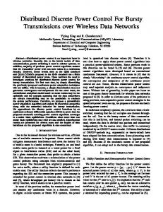
A Manhattan-like System The microcellular system under investigation is a typical metropolitan environment consisting of building blocks of a square shape, as depicted in Figure 1. The cell plan is Asymmetric Half Square (AHS), AHS(1,1), [12]. We assume that the channel assignment is xed and divides the cells into three dierent channel groups (cochannel cells). Thus, resulting in a cluster size of Nc = 3. This cell plan has a line-of-sight (LOS) reuse distance DLOS = 3. In the pictorial presentation in Figure 1, the dark cells represent a single channel group. We further assume that base stations use omnidirectional antennas. 16

In the simulation we use 10  10 cochannel cells, and mobile locations (one per cell) are independently sampled from a uniform distribution over each cell area. The link gain, gij , is modeled as a product of two variables, i.e., gij = lij
sij . The variable sij is the variation in the received signal due to shadow fading; and lij is the large scale propagation loss. We assume that the variables sij 's are independent, log-normally distributed with a mean of 0 dB , and a log-variance of  = 4 dB [7]. Each variable lij depends on the transmitter and receiver locations, and are modeled based on the ndings in [6]. We use a uniform CIR target, t , for all transmitters. We use a greed of power levels D
, which are equally spaced at distance
dB , from 10 log p dB to 10 log p dB . The maximum transmitter power, p, is 1 W (0 dB ), and the dynamic range values are 30 dB and 60 dB . It turns out that there is almost no dierence between the two dynamic ranges, thus only the results for the 30 dB case are presented. Borrowing from GSM and Qualcomm's CDMA systems, we use three values for the grid spacing
, i.e., 0:5; 1 and 2 dB . The receiver noise is taken as 10?15 W (?150 dBW ).

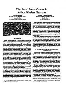
Method of comparison The power vector sequence under the DDPC algorithm converges to p, and under the Ceiling DDPC it may either converge, or oscillate within the envelope Bc (depending on the initial power). Hence, the size of Bc is a good indicator for the power oscillation under the Ceiling DDPC. Note though, that Bc is a random variable governed by the link gain distribution. We use two measures to quantify its size. The rst one is the cumulative distribution function (cdf) of an arbitrary component , taken from f i def = 10 log pi ? 10 log pi j 1  i  N g. The second one is the cdf of max def = max1iN i. The former describes the power dierence for an arbitrary mobile, whereas the latter describes the power dierence for the worst situated mobile. Since power levels are equally spaced with distance
dB , the two cdf's are given by P (  k
) and P ( max  k
), k = 0; 1; 2; : : :, respectively. The impact of the grid size on the mobile outage is evaluated by the outage probability, Poutage = P ( < t ) ; where is the CIR of a randomly selected link. The outage probability measures the long-run proportion of mobiles that cannot be supported. 17

Another practical performance measure is the convergence rate. One of the problems encountered by the continuous DCPC algorithm, is its slow convergence rate when the CIR target is set to support most of the mobiles, and is just below the maximum channel capacity. (This is de nitely a desirable operational value to use.) It turns out from our case study, that spacing the power levels greatly accelerate the convergence, with only a marginal reduction in the outage probability. For our evaluation, we compute an upper bound on the expected convergence time, rather than the actual expected number. The reason is that the convergence time depends on the initial power vector, which is an in nite set. The upper bound is derived as follows. For any given realization, let m1 (m2 ) be the number of power updates required to converge when starting from the all zero (all p) power vector. From Theorem 3.1, it is easy to verify that from any feasible initial power vector, the sequence will enter Bc, after at most m = max(m1 ; m2) number of updates. To evaluate the CIR degradation under Ceiling DDPC at instances where the CIR under DDPC is above the CIR target, we compute the probabilities

P ( < x;   t ) : Here,  is the CIR of a random link under p (i.e., under DDPC); and is its lower bound under Ceiling DDPC (see Lemma 3.5). This cdf measures the lowest CIR level of a random link under the Ceiling DDPC algorithm, in those instances where DDPC can support it. All the statistics above are evaluated via simulation, where under every power control algorithm, we sample 10; 000 instances of mobile locations and shadow fading values. The power updates are made synchronously, and we further

Numerical results Figures 2 and 3 depict the cdf of (i.e., an arbitrary dierence 10 log pi ? 10 log pi ), for various CIR targets (8; 12; 16; 20 dB ) and grid sizes (
= 0:5 and 2 dB ). Observe that the dierence in power is the largest (and therefore so is the potential power oscillation), when the CIR target is around 16 dB . It becomes smaller when it either increases, or decreases. For instance (see Figure 3), when
= 2 dB and t = 16 dB , the transmission power of 20% of the transmitters, will oscillate in a range larger than 2 dB ; 14% of them, in a range 18

larger than 4 dB ; and 8% of them, in a range larger than 6 dB . On the other hand, for

t = 12 dB , the transmission power of 95% of the transmitters will not oscillate at all; for

t = 20 dB , 83% of them will not oscillate. This trend is attributed to the fact that either for small or large CIR targets, the transmission powers are pushed closer to the boundaries, and therefore resulting in a smaller envelope. The aect of the grid size on the envelope size is obvious. Figures 4 and 5 correspond to Figures 2 and 3, for the cdf of max (i.e., the maximum of the dierences 10 log pi ? 10 log pi ). Here, the power potential oscillation statistics re ect only the worst situated mobile. Observe again, that the worst potential oscillation occurs when the CIR target is around 16 dB . Clearly, for that mobile, the potential uctuation is more severe. For instance (see Figure 5), when
= 2 dB and t = 16 dB , the transmission power of the worst mobile will oscillate in a range larger than 4 dB , with probability 0:68; in a range larger than 8 dB , with probability 0:44; and in a range larger than 12 dB , with probability 0:30. On the other hand, for t = 12 dB , its transmission power will not oscillate with probability of 0:41. In Figure 6 we compare between the outage probabilities of the DDPC (with dierent grid sizes) and that of the continuous DCPC. Note that the continuous DCPC is the limiting case of the DDPC, when the grid size approaches zero. (In the simulations we use the dierences of  = 10?2; 10?4 or 10?8, between two consecutive power vectors, as a stopping rule.) The gure illustrates the increase in mobile outage as a result of the power level spacing. This is particularly interesting in light of the gain in the convergence rate which presented in Figure 7. As expected, re ning the power level grid reduces the outage probability. However, a very small CIR gain is obtained by re ning the grid from
= 2 dB to the continuous case. For instance, at the 10% outage probability level, a CIR gain of only 0:5 dB is obtained. The increase in the expected number of update steps however, (Figure 7), is tremendous (from 20 to 160 steps). In general, the expected convergence time under DDPC, is between 2 to 8 times faster compared with the continuous case. The outage probabilities under the optimal DDPC power vector p , and under the power vector p , are also evaluated. That is, under the two extreme power vectors in the envelope Bc. It turns out that they are practically the same. However, as previously noted, it does not imply that the outage probabilities under Ceiling DDPC and under DDPC are the same, 19

as the former may oscillate. The outage reduction under DDPC compared with the Ceiling DDPC is demonstrated by Figure 8. In Figure 8, we observe that for a 16 dB CIR target and a grid of size
= 0:5 dB , 25% of the mobiles are supported under DDPC and not under the Ceiling DDPC. For a grid of size
= 2 dB , 38% of the mobiles are supported under the DDPC and not under the Ceiling DDPC. This gives a substantial advantage to DDPC compared with the Ceiling DDPC. For lower and higher CIR targets, the advantage is smaller.

5 Conclusions We studied transmitter power control algorithms in cellular PCS which use discrete power levels. It is shown that by simply \discretizing" the continuous power control algorithm, the convergence and uniqueness of the continuous power control are lost. The discrete Ceiling DDPC algorithm, is shown to "converge" in a weaker sense, i.e., into an envelope of power vectors rather than to a unique vector. The transmitter powers under this algorithm may oscillate, which results in a poorer link quality and in a higher outage probability. The oscillation is alleviated by the proposed Distributed Discrete Power Control (DDPC) algorithm. Our main conclusions from our case study are the following. First, the size of the convergence envelope Bc depends on the grid size and on the CIR target. It shrinks when the grid is re ned, and it grows when the CIR target becomes closer to a value where the channel capacity is most utilized. Second, the outage probability is marginally reduced by re ning the power level grid. The increase in the expected number of update steps, however, is tremendous. Last, using DDPC reduces the outage probability compared with that of the Ceiling DDPC. The improvement is substantial when the channel capacity is highly utilized.

20

References [1] J. M. Aein. Power Balancing in Systems Employing Frequency Reuse. Comsat Tech. Rev., Vol. 3, No. 2, 1973. [2] M. Almgren, H. Andersson and K. Wallstedt. Power Control in a Cellular System. Proc. IEEE Veh. Tech. Conf., VTC-94:833{837, 1994. [3] M. Andersin, Z. Rosberg and J. Zander. Soft Admission in Cellular PCS with Constrained Power Control and Noise. Proc. 5th WINLAB Workshop, Apr. 1995. [4] M. Andersin, Z. Rosberg and J. Zander. Gradual Removals in Cellular PCS with Constrained Power Control and Noise. IEEE/ACM Wireless Networks, Vol. 2:27{43, 1996. [5] N. Bambos and G. J. Pottie. On Power Control in High Capacity Cellular Radio Networks. Proc. 3rd WINLAB Workshop, Oct. 19-20, 1992. [6] J-E. Berg. A Simpli ed Street Width Dependent Microcell Path Loss Model. COST 231, TD(94)035, 1994. [7] J-E. Berg, R. Bownds and F. Lotse. Path Loss and Fading Models for Microcells at 900 MHz. Proc. IEEE Veh. Tech. Conf., VTC-92:666{671, 1994. [8] G. J. Foschini. A Simple Distributed Autonomous Power Control Algorithm and its Convergence. IEEE Trans. on Veh. Tech., Vol. 42, No. 4, 1993. [9] S. A. Grandhi, R. Vijayan and D. J. Goodman. A Distributed Algorithm for Power Control in Cellular Radio Systems. 13th Annual Allerton Conf. on Commun., Contr. and Computing, Monticello, Illinois, Sept. 1992. [10] S. A. Grandhi, R. Vijayan, D. J. Goodman and J. Zander. Centralized Power Control in Cellular Radio Systems. IEEE Trans. on Veh. Tech., Vol. 42, No. 4, 1993. [11] S. A. Grandhi, J. Zander and R. Yates. Constrained Power Control. Wireless Personal Communications, Vol. 1, No. 4, 1995. [12] M. Gudmundson. Cell Planning in Manhattan Environments Proc. IEEE Veh. Tech. Conf., VTC-92:435{438, 1992. [13] J. C. Lin, T. H. Lee and Y. T. Su. Power Control Algorithm for Cellular Radio Systems. Electronics Letters, Vol.30, No. 3, 195{197, 1994. [14] H. J. Meyerho. Methods for Computing the Optimum Power Balance in Multibeam Satellite. Comsat Tech. Rev., Vol. 4, No. 1, 1974. [15] D. Mitra. An Asynchronous Distributed Algorithm for Power Control in Cellular Radio Systems. Proc. 4th WINLAB Workshop, Oct. 19-20, 1993. 21

[16] R. W. Nettleton and H. Alavi. Power Control for Spread-spectrum Cellular Mobile Radio System. Proc. IEEE Veh. Tech. Conf., VTC-83:242{246, 1983. [17] An Overview of the Application of Code Division Multiple Access (CDMA) to Digital Cellular Systems and Personal Cellular Networks. Document Number EX60-10010, QUALCOMM Inc., May 1992. [18] J. Zander. Transmitter Power Control for Co-channel Interference Management in Cellular Radio Systems. Proc. 4th WINLAB Workshop, Oct. 19-20, 1993. [19] J. Zander. Performance of Optimum Transmitter Power Control in Cellular Radio Systems. IEEE Trans. on Veh. Tech., Vol. 41, No. 1, 1992. [20] J. Zander. Distributed Cochannel Interference Control in Cellular Radio Systems. IEEE Trans. on Veh. Tech., Vol. 41, No. 3, 1992.

22

Wy y

x Wx

Figure 1: The asymmetric AHS(1,1) cell plan with cluster size Nc = 3. The dark crosses are the cochannel cells and the white squares are the buildings seen from above.

Distribution of the difference between power vectors, ∆ = 0.5 dB. 1 0.9 0.8

P( ψ