May 5, 2001 - tangular channel with a width of 50 m, Manning's coefficient n of 0.035, slope of ..... La Houille Blanche, 1, 33â39 (in French). Fugazza, M.
DORA ALGORITHM FOR NETWORK FLOW MODELS WITH IMPROVED STABILITY AND CONVERGENCE PROPERTIES By L. Noto1 and T. Tucciarelli2 ABSTRACT: A new methodology for the solution of shallow water equations is applied for the computation of the unsteady-state flow in an urban drainage network. The inertial terms are neglected in the momentum equations and the solution is decoupled into one kinematic and one diffusive component. After a short presentation of the DORA (Double ORder Approximation) methodology in the case of a single open channel, the new methodology is applied to the case of a sewer network. The transition from partial to full section and vice versa is treated without the help of the Preissmann approximation. The algorithm also allows the computation of the diffusive component in the case of vertical topographic discontinuities, without the introduction of any internal boundary conditions and without any change in the structure of the linear system matrix. The algorithm is tested on one field example, and its performance is compared with the performance of other popular commercial codes.
INTRODUCTION Numerical models play a major role in designing and improving urban drainage networks. Simulation results are widely used for planning, designing, and operational purposes. Many numerical models for the simulation of sewer/channel networks are available today. These can be classified, according to the simplification assumed in the momentum equation, in full dynamic, diffusive, and kinematic models. In the first group one can find models such as SYSTEM11S (S11S) (Abbott et al. 1982; Hoff-Clausen et al. 1982), SWMM-EXTRAN (Roesnerr et al. 1988, HYDROWORKS (HW) (HYDROWORKS 1997), DEMOS (Koussis et al. 1984), MUSS (Fugazza 1993a,b), and SUPERLINK (Ji 1998). S11S is the flow routing module of one of the most popular models of urban sewer systems: MOUSE (Lindberg and Jørgensen 1986). In the second group (diffusive approximation) one finds DEMOS (Koussis et al. 1984), DAVGL-DIFF (Sjo¨berg 1982), and the Akan and Yen model (1981). In the third group (kinematic approximation) one finds ILLUDAS (Chiang and Bedient 1984) and SWMM-TRANSPORT (Metcalf & Eddy, Inc. et al. 1971). Despite the large number of available codes, there are still some difficulties that are not completely solved and can provide limitations in both the accuracy of the solution and the practical handling of real cases. These difficulties have been summarized by Cunge and Mazaudou (1984) in the following points: • The solution requires some approximation when the pipe flow condition moves from partial to full section and vice versa. • The solution can be very slow for networks with a large number of loops. • Small water depths are often encountered in reality. In this case, backwater effects are very important but the use of the complete or the diffusive approximation leads to strong numerical difficulties. • To incorporate manholes and other special manufactures in the network, available algorithms introduce internal boundaries that reduce the efficiency of the original numerical scheme. 1 PhD in Hydr. Engrg., Dept. of Hydr. Engrg. and Envir. Applications, Univ. of Palermo, Viale delle Scienze, 90128 Palermo, Italy. 2 Assoc. Prof., Dept. of Mech. and Mat., Loc. Feo di Vito, 89100 Reggio Calabria, Italy. Note. Discussion open until October 1, 2001. To extend the closing date one month, a written request must be filed with the ASCE Manager of Journals. The manuscript for this paper was submitted for review and possible publication on November 23, 1999; revised November 13, 2000. This paper is part of the Journal of Hydraulic Engineering, Vol. 127, No. 5, May, 2001. 䉷ASCE, ISSN 0733-9429/01/0005-0380–0391/$8.00 ⫹ $.50 per page. Paper No. 22149.
380 / JOURNAL OF HYDRAULIC ENGINEERING / MAY 2001
• Initial dry conditions are often encountered in reality. Once again, some approximation is required in this case to obtain a numerical solution of the problem. Another problem, not mentioned by Cunge and Mazaudou (1984), is that, in some areas with strong ground slope, the sewer pipes can be installed with a similar strong slope. In this case, the channel slope is much larger than the small value allowed by the shallow water hypothesis and the very high Froude numbers can provide instability in the numerical solution. All the models use similar ways to cope with the mentioned problems. To avoid the change from partial to full section (point 1), the models input all the links as either closed channels or pressurized pipes. The geometry of the real section of the closed channels is then slightly changed by introducing the so-called ‘‘Preissmann slot’’ (Cunge and Wegner 1964), which gives a minimum width to all the flow sections, even for water levels above the real closed channel contour. This allows the computation of very small storage volumes and very large wave celerity. The Courant number restriction gives a lower bound to the size of the Preissman slot, and it shall be shown that an evident artificial reduction of the maximum flow in a given section can result from its use. Most of the models use the double sweep method (DSM) to solve at each time step the banded linear system resulting from the discretization of an open network (Abbott 1979). To cope with networks closed by a large number of loops (point 2), the SUPERLINK (Ji 1998), SWMM-EXTRAN, and CAREDAS (Cunge and Mazaudou 1984) models divide the nodes and the links into two groups. The first group is given by the nodes and the links internal to a single reach or to an open part of the network, whereas the second group is given by the junction nodes that close the loops of the network. The solution is found in two different steps. First the DSM is applied to find the solution of the open network formed by the first group of nodes and links, then a smaller (not banded) system is solved to adjust the value of the unknowns at the junction nodes. Other authors, such as Kao (1980), Joliffe (1984), and Sen and Garg (1998), searched for an efficient way of numbering the nodes to solve simultaneously the system of equations and unknowns. Difficulties of points 3 and 5 arise at the wavefront when the particle velocity is subcritical or the diffusive approximation is applied (Tucciarelli and Termini 2000) and may be circumvented by the addition of a nominal ‘‘base flow’’ defined as the normal flow at a prescribed base depth in a conduit. For example in HW, base depth is equal to 5% of the conduit height. This results in a base flow of 1.9% of pipe full capacity for circular pipes and 5% for rectangular ones.
One of the most common structures found in sewage networks is the manhole, which is often placed in the sewer to allow a slope of the channel smaller than the ground slope (drop manhole). The location of a manhole at a node can imply that the bottom of the ends of the two channels sharing the same node have different topographic elevations. This requires the introduction of two different water levels at the same node and the use of a corresponding internal boundary condition (point 4). If many manholes are used, the computational efficiency provided by the DSM method can be lost. Finally, a strong channel slope can correspond to very high Courant numbers, and in this case, the use of explicit methods, similar to all the shock capturing schemes, requires the use of a very small time step (this is very disturbing because the kinematic condition is almost immediately attained in these cases). If diffusive models are used, numerical instabilities arise, especially for small initial water depths. In the following, a new numerical algorithm for the simulation of an urban drainage network is proposed. The algorithm has the merits of being unconditionally stable and having the ability to cope with all the mentioned problems without any special expedient. An important issue is the choice of neglecting the inertial terms in the momentum equation, to obtain the so-called diffusive model. This model normally is more accurate than the quasi-steady dynamic model, because usually during the rising part of the hydrograph, the local acceleration is positive and the convective acceleration is negative. The opposite takes place during the falling part of the hydrograph when a compensation for the error in dropping these terms can be observed. The choice of diffusive model has the advantage of reducing the actual number of unknowns to the number of nodes, improving the stability of the solution, allowing the use of larger Courant numbers, and most important, simplifying the external and internal boundary conditions of the model. Validity of the diffusive model fails when inertial terms are more relevant than resistance terms, such as immediately after the sudden opening of a gate in an open channel or in the computation of waves that have a length smaller than the channel dimension. The difference between the results of the dynamic and the diffusive models also becomes important when shock waves, generated during heavy storms or as a result of control device operation, propagate along the channel. However, in the common case of a channel with a closed section, two-phase flow occurs and this causes pressure changes in the air phase entrapped in the conduit (Cardle and Song 1988). According to Trajkovic et al. (1998), experimental investigations are still required to better understand the interaction between air and water during transition and to consequently develop, for the simulation of these phenomena, more reliable numerical models. In all the other cases, the price to pay is some difference in the solution with respect to the one computed by the dynamic model. However, in field applications, inadequate information on junction losses and data error cause uncertainties far exceeding the small accuracy that can be gained by using the dynamic model. Indeed, according to Yen (1987), the junction losses are quite significant in comparison to the sewer pipe losses, and, therefore, improper accounting for these losses would render any sophisticated sewer routing inaccurate and meaningless. Besides this, even if only a few of the available models are diffusive, the other ones apply some simplification of the momentum equation to cope with the above listed problems. The S11S model uses the kinematic approximation in the momentum equation for supercritical flows; the SWMMEXTRAN model discretizes the flow rate in each link of the network with a constant value, introducing a larger error in the estimation of the flow rate spatial derivatives; and HW
reduces the weight of the kinetic energy from 1 to zero when the Froude number increases from 0.8 to 1.0. SOLVING 1D SAINT-VENANT EQUATIONS USING DORA (DOUBLE ORDER APPROXIMATION) SOLVER The sewer system is idealized as a series of links or pipes that are connected at nodes or junctions. Links and nodes have well-defined properties that, taken together, permit representation of the entire sewer system. Although links transmit flow from node to node, nodes are the storage elements of the system and some of these can correspond to manholes or pipe junctions in the physical system, or more frequently, to simple computational nodes. The variables associated with a node are storage volume, hydraulic head, and surface area. The storage volume of the node at any time is equal to the sum of the water volume in the half-pipe lengths linked to the same node and the water volume in the manhole or in the pipe junction. The final system of differential equations for the sewer flow problem is derived from the gradually varied, 1D unsteady flow equations for open channels, which in the diffusive approximation, can be written in the form L
⭸H ⭸q ⫹ ⫺Q=0 ⭸t ⭸x
(1)
⭸H q兩q兩 = ⫺ 2 2 4/3 ⭸x cR
(2)
where L, H, h, , R, Q, c, and q represent respectively the channel width, water surface elevation, water depth, cross-sectional area, hydraulic radius, entering flux, Strickler roughness coefficient, and flow rate. The basic idea of the DORA algorithm is to split the surface elevation H and the flow rate q in the sum of two components and to solve each of them using different approximation orders. Using the following notation: H = H p ⫹ hc;
Eqs. (1) and (2) become L
冉
冊
⭸hc ⭸H p ⫹ ⭸t ⭸t
⫹
q = q p ⫹ qc
⭸qc ⭸q p ⫹ ⫺Q=0 ⭸x ⭸x
⭸hc ⭸H p 兩 qc 兩 (qc ⫹ 2q p) ⫹ ⬵ ⫺ 2 c 2 c 4/3 ⭸x ⭸x c ( ) (R )
(3)
(4) (5)
where c and R c = section area and hydraulic radius, respectively, corresponding to the water depth hc . The approximation in (5) holds if the first component of the discharge is small with respect to the second one and H p ⫺ z is small with respect to hc, where z is the channel bottom elevation. The functions hc and qc are the water depth and the flow rate, respectively, computed by solving the kinematic problem ⭸hc ⭸qc ⫹ ⫺Q=0 ⭸t ⭸x
(6)
⭸H n qc 兩 q c 兩 = ⫺ 2 c 2 c 4/3 ⭸x c ( ) (R )
(7)
L
where H n = total water level at the known time level t n, assumed constant along the new time step. Eqs. (6) and (7) are integrated from time t n to time t n⫹1 = t n ⫹ ⌬t, with initial conditions hc = h n
(8)
n
where h = water depth at the known time level. Observe that (4) and (5) approach (1) and (2) for ⌬t → 0. JOURNAL OF HYDRAULIC ENGINEERING / MAY 2001 / 381
depth [h ci (t n⫹1) ⫹ h in]/2. The average flux entering cell k from cell i is given by
After the solution of the kinematic problem, the remaining components of H and q in (3) can be computed at the time level t n⫹1 by solving (4) and (5) with a fully implicit finitedifference scheme. These components are called parabolic. Because systems (4) and (5) and (6) and (7) are solved using two different approximation orders for the water levels, the overall algorithm is called DORA, that is, the acronym of Double ORder Approximation.
To obtain a numerical solution for (6) and (7), each pipe (or channel) is divided into one or more computational links, and connecting nodes, and into several cells given by the two half links sharing the same node (Fig. 1). If more than one channel forms a network, each cell is given by the sum of the halves of each link sharing the same node. The water depth is assumed to be constant in space inside each cell of the channel; the flow rate leaving a cell from nodes i to j is a function of the water level gradient computed at the end of the previous time step in the link from nodes i to j (constant during the new time step) and of the water depth in node i (variable during the new time step). According to the previous hypothesis, the momentum and continuity equations [(6) and (7)] can be combined, in each cell, in one ordinary differential equation
冘 j=1
dh ci Fl = Ai (h ) ⫹ dt e ji
c i
冘
c i
Fl (h ),
i = 1, 2, . . . , N
Ne
j=1
Solution of Parabolic Problem After computation of the kinematic water depths, system (4) and (5) can be written in the form
k=1
冎
⭸H p ⭸q p ⭸hc ⭸qc ⫹ = ⫺L ⫺ ⫹Q ⭸t ⭸x ⭸t ⭸x
冘
H pi = zi,
⌬t
n i
Fl (h ) (10)
q pij = ⫺␣ij
(15)
冉
冉冘 Mi
j=1
冊
␣ij Ai ⫹ ⌬x ⌬t
n j
冘 Mi
H ip ⫹
⫺ (H ⫺ H )] n i
冊
H pj ⫺ H pi h cj ⫺ h ic H jn ⫺ H in ⫹ ⫺ ⌬x ⌬x ⌬x ␣ij =
382 / JOURNAL OF HYDRAULIC ENGINEERING / MAY 2001
i = 1, . . . , N
where zi = bottom level of the channel at node i. The final set of algebraic equations is given by
where Ai = area computed as function of the average
Approximation Order of Kinematic and Parabolic Components
(14)
Solution of the kinematic problem has been found assuming a water depth constant in space inside each cell. To compute the solution of problems (13) and (14) using a fully implicit finite-difference scheme, the gradients of the kinematic water depths have to be estimated at time level t n⫹1 . This is done by assuming a linear variation of the heads between two nodes connected by a link and a constant flow rate inside each link, which is a function of the average link water depth. This change does not affect the total mass of the system and is equivalent to moving from a zero-order to a first-order approximation of the heads. Computation of the kinematic flow rate gradients can be avoided by observing that the right-hand side of (13) is equal to the opposite of the left-hand side of (6) and can be neglected. Using a standard finite-element scheme in fully implicit form (Gambolati 1994), (13) and (14) can be discretized with a system of N equations in the N parabolic water level nodal unknowns. The initial value of the unknowns, at time t n, is
Nu
u ij
(13)
⭸H p 2 兩 qc 兩 ⭸hc ⭸H n ⫹ 2 c 2 c 4/3 q p ⬵ ⫺ ⫹ ⭸x c ( ) (R ) ⭸x ⭸x
Fl uik(h ni )
Fl eji ⌬t ⫺ Ai [h ci (t n⫹1) ⫺ h ni ]
j=1
FIG. 1.
(12)
Observe that (9) has no singularity for h ci = 0 and can also be solved if the initial value of the water depth is zero. Moreover, the above algorithm has been proven by means of Fourier analysis to be unconditionally stable in the linear case, for example, in the solution of the ground-water convective transport problem (Tucciarelli and Fedele 2000). In this case, not linear, unconditional stability has been empirically observed in several 1D and 2D applications (Tucciarelli and Termini 2000).
(9)
1. Order the nodes according to the water level value H at time t n (beginning with the highest and ending with the lowest one). 2. For each cell i, solve (9) from time level t n to time level t n⫹1 with any required precision using, for example, a Runge-Kutta numerical integration (Press et al. 1988). Observe that in the first cell there are no fluxes entering from other cells. 3. After solution of (9), the average flux leaving cell i toward cell k can be computed from the mass balance
再冘
q cik(t n⫹1) = Fl uik(t n⫹1)
L
where N = total number of nodes (and cells); Fl eji = average flux entering in cell i during the time step from any of the Ne connected nodes with higher total head; Ai (h ic) = horizontal water surface area of cell i; h ci = water depth in node i; and Fl uik(h ci ) = flux leaving cell i toward any Nu connected node with a lower total head. Observe that to solve each (9) in the h ci variable, the average fluxes on the left-hand side have to be known. This can be accomplished in the following way:
Fl uik =
and the kinematic flow rate, in the link between nodes i and k at time t n⫹1, is equal to
Nu
u ik
(11)
4. Move to the next cell, until (9) is solved for the cell with the lowest water level.
Solution of Kinematic Problem
Ne
Fl eik = Fl uik
j=1
ccij (R ijc )2/3兹⌬x
兹2 兩 H jn ⫺ H in 兩
␣ij p Ai Hj = zi ⫺ ⌬x ⌬t
(16) (17)
冘 Mi
j=1
␣ij [(h ic ⫺ h jc) ⌬x (18)
where the kinematic water depths are estimated at time level t n⫹1; and Mi = number of the nodes linked to node i. The linear system [(18)] has a matrix that is symmetric and positive definite. Using a standard finite-difference methodology, the non-
zero coefficients of the matrix can be stored in a vector format and the system solved using the conjugate gradient method (Gambolati 1994). The total nodal water level at node i and the flow rate at link ij at time t n⫹1 = t n ⫹ ⌬t are finally given by H n⫹1 = H ip(t n⫹1) ⫹ h ic(t n⫹1) i q
n⫹1 ij
c ij
= q (t
) ⫹ q (t
n⫹1
p ij
(19a)
n⫹1
)
(19b)
To obtain, a prescribed stage hydrograph, h* = h(t), at the downstream boundary nodes, the solution of the system at these nodes is forced to be H p = z ⫹ h* ⫺ hc
(20)
To obtain a prescribed water level gradient (‘‘kinematic’’ downstream boundary conditions) at the same nodes, the lefthand side in (7) is changed with the prescribed gradient and the parabolic component of the leaving flux is neglected [which is equivalent to leaving (18) unchanged]. The main advantage of the DORA algorithm is that the solution of the parabolic problem [(18)] is usually not very far from the initial value of the parabolic component (that is, the channel bottom elevation) and only requires, in (17), a minimum gradient of the total initial water level. The solution of the kinematic problem, which can be thought of as a prediction of the unknowns at the end of the time step, is very robust and can also be found when the initial water depth is zero or when the time step is very large (Tucciarelli and Fedele 2000). Internal Boundary Conditions and Junction Head Losses One feature of the DORA method is easy accommodation of internal boundary conditions. These conditions could occur when two or more conduits are connected in a manhole at different topographic elevations. The bottom of each of these conduits can be either submerged [Fig. 2(a)] or not submerged [Fig. 2(b)] by the water level at the manhole. According to the assumptions of the diffusive model, the water level is the same for both the link and the manhole in the first case and different in the second one. In this last case the water level at the end of the link is equal to the junction topographic level and is higher than the water level in the manhole. This implies that, moving from the first case to the second case, a new mode should be added and the water level in the two nodes located at the same planar position should
FIG. 2.
Manhole In-Out Conditions
FIG. 3.
be linked by the mass continuity equation. This requires a change of the structure of the linear system solving the diffusive problem, as well as the loss of the symmetry of the corresponding matrix. In the DORA procedure, this inconvenience can easily be solved. For the sake of simplicity, assume first that two computational links are connected with a manhole at different elevations (Fig. 3). Call zA, zB, zC, and zD the elevations of the ends of the computational links A-B (connected at the higher topographic elevation) and C-D. Assume that B and C are at the opposite ends of the manhole (identified as node m) and that Hm is the elevation of water surface in the manhole. If zC < Hm < zB (case II) at the beginning of the new time step, DORA solves the kinematic problem, neglecting the water storage in the half of the link A-B connected to B and using the topographic elevation zB to compute the piezometric gradient in the link A-B (Strelkoff and Katopodes 1977). To compute the solution at the end of the time step, it is now sufficient to neglect the parabolic component of the flow rate in the A-B link. This can be done by computing the matrix coefficients as the sum of the contribution of each link and by neglecting the contribution of the links where the topographic elevations of at least one end is higher than the water level at the corresponding node. If Hm < zC (case III), the average flux leaving from node m is equal to zero. A similar methodology can be followed when several links are connected to the same node at different levels. The head losses in the manhole should be neglected according to the hypothesis of the diffusive approximation. This could provide a not-negligible error if a large number of manholes is present, especially if the connected links are in surcharged conditions. A large uncertainty exists about the estimation of these head losses. Assuming one of the available experimental expressions, it is easy to incorporate these in the DORA model. For example, according to HW, assume the head loss ⌬hm in the manhole to be equal to ⌬hm = K
v 20 2g
(21)
where v 0 = normal velocity corresponding to the flow rate q at the junction with the upstream link; and the loss coefficient K is given as a function of the ‘‘surcharge ratio,’’ defined as SR = hB /DV, where DV is the vertical dimension of the upstream link (Fig. 4). The head loss is applied by assigning in the upstream link an additional pseudoroughness providing the same head loss computed by (19), using the water levels and the flow rate at the beginning of the new time step. A similar procedure is applied in the case of a three- or four-way junction. Observe that the head loss in a manhole is set equal to zero in cases II and III of Fig. 3 because of the zero value of the surcharge ratio.
Computational Scheme of Internal Boundary Conditions JOURNAL OF HYDRAULIC ENGINEERING / MAY 2001 / 383
FIG. 4.
Headloss Curve [by HYDROWORKS (1997)]
TESTING DORA MODEL AGAINST SOME LITERATURE CASES To test the performance of the proposed DORA model, the same is applied to some cases selected from the literature. The first case is taken from Abbott et al. (1982). A 9,150-m-long pipe with diameter d = 1.82 m, slope i = 0.001, and Strickler coefficient c = 80 m1/3/s initially carried a discharge of 0.8 m3/s. The inflow at the upstream end, as a function of time, is shown in Fig. 5, and the ‘‘free outflow’’ was assumed to be the downstream boundary condition. Fig. 5 also shows the outflow hydrographs obtained by Abbott et al. (1982) using the S11S and the method of characteristics, along with the outflow hydrographs obtained by the writers using DORA and HW. The space and time interval, ⌬x and ⌬t, used for these models are equal to 260 m and 150 s. The first two codes, which are fully dynamic, compute a peak of the discharge that is slightly higher, but the other two compute hydrographs that are quite similar, even if HW is fully dynamic for Courant numbers ⌬t holds, assume hc = htop and save the volume ⌬Fi = (⌬t e ⫺ Tf ) 兺Nj=1 Fl eji for the following diffusive problem. In this problem, add the ⌬Fi /⌬t flow rate as the entering flux in node i. A similar procedure can be used in the case of hmax < htop < hn or hmax < hn < htop. Observe that the solution of several differential equations [(9) and (22)] is required only for nodes where the transition from partial to full section or vice versa is in progress. This allows a very small increase of the total computational time. To test the proposed algorithm in the process of transition, the same pipe used in the second test (with a slope equal to 0.001), has been used. This pipe, characterized by a maximum normal discharge of 0.049 m3/s, is affected by the triangular inflow hydrograph shown in Fig. 12, characterized by a peak discharge of 0.2 m3/s. In Fig. 12 the outflow hydrographs computed by DORA and HW are compared. The phenomenon of surcharging begins at time T1 when, in the first upstream computational link, total water level exceeds pipe crown; at time T2 all the pipe is surcharged and remains so up to the time T3, for a period Tp equal to 500 s. During this period the proposed model computes an outflow hydograph that is quite similar to the entering one. This, of course, honors the mass conservation equation according to the assumption of incompressible water. SOLVING CASE OF LOOPED CHANNEL NETWORKS To test the performance of the proposed DORA model in the case of looped networks, the trial network system of Ji (1998) was used. The network, shown in Fig. 13, is formed
FIG. 10.
Comparison of Hydrographs Computed with Four Different Models
JOURNAL OF HYDRAULIC ENGINEERING / MAY 2001 / 387
TABLE 2. Ji (1998) ID channel 1 2 3 4 5 6
FIG. 11.
Relationship q = q(h) for Circular Pipe
by six links, six nodes, and one closed path. The network’s characteristics are listed in Table 2. The network is subject to two inflow boundary conditions (nodes A and C) and two stage boundary conditions (outflow nodes D and F). Fig. 14 shows inflow hydrographs and stage hydrograph imposed at bound-
FIG. 12.
General Characteristics of Example Channel Network of Length (m) 300 300 300 500 410 310
Slope 1 1.3 1.7 6 2 3.25
⫻ ⫻ ⫻ ⫻ ⫻ ⫻
10⫺3 10⫺3 10⫺3 10⫺4 10⫺3 10⫺4
Diameter (m)
Manning (s/m1/3)
0.800 0.500 0.500 0.500 0.500 0.500
0.01429 0.01429 0.01429 0.01429 0.01429 0.01429
ary conditions. There was no base flow imposed on the network, and because of the elevation of nodes D and F, pipes 3 and 5 are affected by reversal flow due to the rising stage hydrograph. Outflow hydrographs, computed by the DORA model and shown in Fig. 15, are compared with those computed by Ji (1998). The two hydrographs are quite similar, even if Ji’s model is fully dynamic. The largest difference can be observed during the descending limb of the inflow hydro-
Case of Surcharged Channel: Comparison of Outflow Hydrographs Computed by HW and DORA Model
FIG. 13.
Scheme of Example Channel Network of Ji (1998)
388 / JOURNAL OF HYDRAULIC ENGINEERING / MAY 2001
FIG. 14.
FIG. 15.
Boundary Conditions
Comparison of Outflow Hydrographs
graph, when a change in the outflow hydrograph slope can be due to the arrival of reflection waves. The diffusive model provides a bad estimation of both the intensity and the speed of these waves and a larger error is evident. APPLICATION TO REAL CASE: NETWORK OF CASCINA SCALA The DORA model was used to simulate the flow through the experimental sewer system sited in Pavia (north of Italy). The urban catchment that contains this sewer system covers an area of 11.3 ha, of which 65% is impermeable. The geometric and topographic data are well known from direct measurements. The good knowledge of the geometry allows one to make some more detailed considerations on the computed hydraulic behavior of the drainage network. The network used for the simulation is shown in Fig. 16. This network is composed of 19 nodes, 18 circular and egg-shaped links with a slope from 0.2 to 1.0%. All nodes, shown in Fig. 16, represent manholes and inflow points. Some of these are three-way or four-way junctions and are also characterized by pipe linked
to the manholes at different elevations. The discharge results were compared with results of the simulation computed by HW using the same network links and nodes under the same inflow hydrographs. The DORA model simulations rely on the inflow hydrographs, which were predicted using the runoff module of HW according to the rainfall record. Fig. 17 shows, in addition to the hydrograph measured in the outlet node, the comparisons of the outflow hydrographs computed by the two mentioned models. A good agreement between these models can be observed, whereas the measured hydrograph is different because of the large errors in the estimate of the inflow hydrographs. The run time for DORA on a IBM compatible 350-MHz computer was 13 s for a 12-h simulation with a time step of 1 min and 74 computational nodes, and run time for HW was 10 s, with the same simulation and the number of nodes equal to 42. A similar difference (20–25%) between the computational times of DORA and HW has been observed in all simulated events. A systematic comparison between the computational speed of DORA and of the available commercial codes has not been performed. JOURNAL OF HYDRAULIC ENGINEERING / MAY 2001 / 389
FIG. 16.
FIG. 17.
Network of Cascina Scala Catchment
Comparison of Outflow Hydrographs for DORA Model and HW
CONCLUSIONS A new algorithm for the simulation of unsteady-state flow in sewer systems has been developed. The algorithm has been called DORA and is based on the decomposition of the equation state variables in two components. The first component, called kinematic, is computed using a zero-order approximation of both the flow rates and the water levels; the second component, called parabolic, is computed assuming a first-order approximation of the water levels and solving a standard parabolic finite-difference model. In this paper several advantages of the methodology are discussed, including the accommodation of the transition from free-surface flow to pressurized flow without the use of the Preissman slot or the use of very strong channel slopes. The choice of using the diffusive form is motivated by the observation, documented in this paper with the application of both diffusive and dynamic models to several examples, that the difference between the results of the two types of models is negligible in most of the cases of practical interest and, according to the experience of the writers, far beyond the error due to other sources of uncertainty. REFERENCES Abbott, M. B. (1979). Computational hydraulics. Element of the theory of free surface flows, Pitman Publishing, Ltd., London. Abbott, M. B., Havnø, K., Hoff Clausen, N. E., and Kej, A. (1982). ‘‘A 390 / JOURNAL OF HYDRAULIC ENGINEERING / MAY 2001
modelling system for the design and operation of storm-sewer networks.’’ Engineering applications of computational hydraulics. Vol. 1: Homage to Alexander Preissman, Abbott and Cunge, eds., Pitman Publishing, Ltd., London, 11–39. Akan, A. O., and Yen, B. C. (1981). ‘‘Diffusion-wave flood routing in channel networks.’’ J. Hydr. Div., ASCE, 107(6), 719–732. Cardle, J. A., and Song, C. C. S. (1988). ‘‘Mathematical modeling of unsteady flow in storm sewers.’’ Int. J. Engrg. Fluid Mech., 1(4), 495– 518. Chiang, C. Y., and Bedient, P. B. (1984). ‘‘Simplified model for a surcharged stormwater system.’’ Proc., 3rd Int. Conf. on Urban Storm Drainage, 387–396. Cunge, J. A., and Mazaudou, B. (1984). ‘‘Mathematical modelling of complex surcharge systems: Difficulties in computation and simulation of physical situations.’’ Proc., 3rd Int. Conf. on Urban Storm Drainage, 363–373. Cunge, J. A., and Wegner, M. (1964). ‘‘Integration numerique des equations d’ecoulement de Barre de Saint-Venant par un schema implicite de differences finies: Application au cas d’une galerie tantot en charge, tantot a surface libre.’’ La Houille Blanche, 1, 33–39 (in French). Fugazza, M. (1993a). ‘‘A software system for runoff and routing modelling in drainage catchments.’’ Proc., 6th Int. Conf. on Urban Storm Drainage, 230–236. Fugazza, M. (1993b). ‘‘Theoretical development of a mathematical model for operation and design of hydraulic channel network.’’ Proc., 6th Int. Conf. on Urban Storm Drainage, 275–281. Gambolati, G. (1994). Lezioni di Metodi Numerici per Ingegneria e Scienze Applicate, Ed. Libreria Cortina, Padova (in Italian). Hoff-Clausen, N. E., Havnø, K., and Kej, A. (1982). ‘‘System 11 sewer —A storm sewer model.’’ Urban stormwater hydraulics and hydrology, B. C. Yen, ed., Water Resources Publications, Littleton, Colo., 137– 146.
HYDROWORKS DM 3.03: Help on line. (1997). Wallingford Software Ltd. and Anjou Recherche. Ji, Z. (1998). ‘‘General hydrodynamic model for sewer/channel networks systems.’’ J. Hydr. Engrg., ASCE, 124(3), 307–315. Joliffe, I. B. (1984). ‘‘Free surface and pressurized pipe flow computation.’’ Proc., 3rd Int. Conf. on Urban Storm Drainage, 397–405. Kao, K.-H. (1980). ‘‘Improved implicit procedure for multi-channel surge computation.’’ J. Can. Soc. of Civ. Engrs., 7, 505–512. Koussis, D., Bowen, J. D., and Zimmer, D. T. (1984). ‘‘DEMOS: A diffusive model simulator.’’ Proc., 3rd Int. Conf. on Urban Storm Drainage, 483–492. Lindberg, S., and Jørgensen, T. W. (1986). ‘‘Modelling of urban storm sewer systems.’’ Proc., Int. Symp. on Comparison of Urban Drainage Models with Real Catchments Data, UDM ’86, 171–184. Metcalf & Eddy, Inc., University of Florida, Water Resources Engineers, Inc. (1971). ‘‘Storm water management model.’’ Water Pollution Control Res. Ser., 11024 DOC, Vols. 1–4, U.S. EPA, Washington, D.C. Press, W. H., Flannery, B. P., Teukolsky, S. A., and Vetterling, W. T. (1988). Numerical recipes, Cambridge University Press, Cambridge, U.K.
Sen, D. J., and Garg, N. K. (1998). ‘‘Efficient solution technique for dendritic channel networks using FEM.’’ J. Hydr. Engrg., ASCE, 124(8), 831–839. Sjo¨berg, A. (1982). ‘‘Sewer network model DAGVL-A and DAGVLDIFF.’’ Urban stormwater hydraulics and hydrology, B. C. Yen, ed., Water Resources Publications, Littleton, Colo., 127–136. Strelkoff, T., and Katopodes, N. D. (1977). ‘‘End depth under zero-inertia conditions.’’ J. Hydr. Div., ASCE, 103(7), 699–711. Tang, X.-N., Knight, D. W., and Samuels, P. G. (1999). ‘‘Volume conservation in variable parameter Muskingum-Cunge method.’’ J. Hydr. Engrg., ASCE, 125(6), 610–620. Trajkovic, B., Ivetic, M., Calomino, F., and D’Ippolito, A. (1998). Proc., 4th Int. Conf. on Developments in Urban Drainage Models, 279–286. Tucciarelli, T., and Fedele, F. (2000). ‘‘An efficient double order solution of the groundwater contaminant transport problem.’’ Proc., 13th Int. Conf. on Computational Methods in Water Resour. Tucciarelli, T., and Termini, D. (2000). ‘‘Finite-element modeling of floodplain flows.’’ J. Hydr. Engrg., ASCE, 126(6), 416–424. Yen, B. C. (1987). ‘‘Urban drainage hydraulics and hydrology: From art to science.’’ Proc., 4th Int. Conf. on Urban Storm Drainage, 1–24.
JOURNAL OF HYDRAULIC ENGINEERING / MAY 2001 / 391